
A Single-Anchor Cooperative Positioning Method Based on Optimized Inertial Measurement for UAVs


College of Intelligence Science and Technology, National University of Defense Technology, Changsha 410073, China
*
Author to whom correspondence should be addressed.
Drones 2023, 7(9), 577; https://doi.org/10.3390/drones7090577
Submission received: 21 August 2023
/
Revised: 10 September 2023
/
Accepted: 11 September 2023
/
Published: 13 September 2023
Abstract
:Benefiting from its structural simplicity and low cost, the inertial/ranging integrated navigation system is widely utilized in multi-agent applications, particularly in unmanned aerial vehicles (UAVs). As the deployment of UAVs in complex environments becomes more prevalent, accurate positioning in sparse observation scenarios has become increasingly important. In satellite-denied environments with few anchors, traditional filtering methods for positioning suffer from poor effectiveness due to the lack of constraints. This article proposes a method to enhance positioning accuracy in such environments by optimizing the inertial outputs of each UAV. The optimization process is based on the range measurements between the UAVs and a single anchor. By solving the optimization function derived using Bayesian theory, the optimized inertial outputs of the UAVs can be obtained. These optimized inertial data are then used in place of the original measurements for position estimation in the filter, resulting in improved performance. Simulation and real-world experiments validate that the proposed method can enhance UAVs’ positioning accuracy in single-anchor environments, surpassing the performance of a single optimizer or filter. Furthermore, the positions estimated by cooperative agents demonstrate higher accuracy than those estimated by individual agents, as more ranging measurements are incorporated.
1. Introduction
In recent years, multi-agent systems have found increasing applications in various fields such as military, agriculture, and commerce, especially for multi-UAV systems. One critical requirement in these systems is accurate positioning. The ranging-based positioning method has emerged as a common solution, thanks to the availability of cost-effective and high-efficiency range sensors. Among the range sensors commonly used in such systems, ultra-wideband (UWB) modules [1] have gained significant popularity. These modules have been extensively utilized in UAVs due to their high-ranging accuracy, anti-multipath capabilities, and low power consumption [2].
The agents equipped with UWB modules can receive range measurements from fixed anchors which have predetermined locations. These range measurements from the anchors play a crucial role in providing geometric constraints and approximate position estimations for the agents. This methodology is akin to the three-ball intersection positioning technique used for satellites. It proves particularly useful in environments where a Global Navigation Satellite System (GNSS) is unavailable or unreliable, such as indoor spaces like rooms [3], underground coal mines [4], underwater environments [5,6], and other similar settings. In many research studies on ranging-based positioning systems, the principles of graph optimization [7,8,9] or Kalman filtering [10,11] are commonly employed to track the position of the agent. In some cases, a sliding window approach [7] is also incorporated to enhance trajectory smoothness. These techniques enable accurate and reliable position tracking in multi-agent systems utilizing range measurements. However, relying on a single ranging source is typically inadequate for achieving precise positioning due to the inherent limitations of ranging, such as susceptibility to sudden changes or interruptions, as well as the low frequency of measurements.
Fusing the inertial sensor and the range sensor is a prevalent approach to enhancing positioning accuracy. The high-frequency inertial measurements include angular velocities and specific forces. The inertial calculation process can transform the measurements in the body frame to the position in the navigation frame. Due to the accumulation of inertial errors, the positioning accuracy continuously decreases over time, and the range measurements can provide constraints and eliminate the influence of errors. In contrast to utilizing range measurements alone, the integration of inertial sensors enables more precise estimation of the motion dynamics model of the system [12]. By incorporating inertial calculations, the integration process establishes a correlation between the motion states of both preceding and succeeding moments in time, and it allows for a more comprehensive prediction of the navigation state [13].
The positioning method that integrates UWB and Inertial Measurement Unit (IMU) shares significant similarities with simple UWB positioning techniques, primarily involving optimization and filtering methodologies. The optimization methods primarily rely on the graph optimization model [14]. The sliding window technique [15] is often employed to estimate relative positions at selected key points by combining distance measurements with acceleration estimates. The filtering methods are mainly based on the Kalman filter [16], which linearizes the nonlinear ranging to predict and update the navigation state of the agent. The current research on nonlinear filtering integrating UWB and IMU mainly focuses on Extended Kalman Filter (EKF) [12,17], Unscented Kalman Filter (UKF) [18,19], and Invariant Extended Kalman Filter (IEKF) [20]. These combined approach leverages the advantages of both range and inertial measurements to enhance the accuracy and robustness of the positioning system.
In a multi-agent system, agents equipped with IMUs can receive range measurements from not only the anchors but also other agents. This is a common pattern of cooperative positioning. The additional range measurements can enhance the positioning accuracy of cooperative agents [21,22,23], compared to the single-agent positioning method.
Whether it is single-agent positioning or multi-agent cooperative positioning, the majority of inertial-ranging positioning methods are built upon multi-anchor networks. These methods rely on the presence of open space and stable communication channels to facilitate ranging [24]. In practical application environments, there may not be enough anchors or the communication is sometimes restricted, and it is not always possible to receive enough signals from multiple anchors at the same time. Therefore, it is important to explore improved positioning methods in sparse anchor environments, where single anchor positioning [25] is the most fundamental case.
The traditional single-anchor positioning methods build virtual anchors for positioning [26,27]. Some methods also involve additional measurements such as velocities [28] and angles [29]. Recently, a geometry-based single-anchor positioning method introduced in [30] estimated the position only by inertial and range measurements. Another research proposed in [31] improved the accuracy of velocity estimation without the same sensors. Our group has also presented an optimization-based positioning method for single-anchor positioning [32]. Different from the other methods, we aim at the cooperation of the agents. The proposed method involves the range measurements between agents in the process of building constraints, which centrally improve the positioning accuracy of the agents, compared to the positioning of individual agents.
The main contributions of this paper include the following:
- 1.
- We propose a cooperative positioning method in single-anchor environments based on range and inertial measurements. At the moments of range observation, an optimizer provides the optimized inertial data to a filter, and the filter outputs the position using the prior navigation state of the agent.
- 2.
- An optimization method for inertial measurements in a multi-agent system is presented. The optimal estimation model is derived from Bayesian theory, and the optimal inertial measurements are obtained at the extreme points, whose existence is further discussed.
- 3.
- The performance of the single-anchor cooperative positioning method is presented in a simulated multi-UAV environment and a real-world indoor environment. The impact of cooperation on improving the positioning accuracy is also discussed.
The rest of this paper is organized as follows. The preliminaries and sensor models are presented in Section 2. Section 3 introduces the process of cooperative positioning method, where we focus on the derivation of the optimization algorithm. Section 4 and Section 5 evaluate the simulation and real-world experimental results, respectively.
2. Preliminaries and Sensor Models
The sensors involved in the multi-agent system consist of inertial sensors and range sensors. Before the optimization, the error distribution of the sensor outputs need to be determined first.
2.1. Inertial Sensor Model
The composition of inertial errors is complex, and there are various approximate models for sensors with different accuracies. According to IEEE standards for inertial devices in [33], the main errors that may exist in inertial sensors include random walk, quantization noise, correlated (Markov) random drift, bias instability, and ramp instability. This classification of errors is detailed based on the characteristics of noise, but there is a significant difference in the magnitude of these errors. The classification of inertial errors based on static and dynamic components introduced in [34] is widely accepted for high-accuracy sensors, but it is not available for low-accuracy and medium-accuracy sensors.
Referring to the classification methods in [33,34], the classification of inertial errors in this paper is given in Figure 1.
As shown in Figure 1, the inertial errors can be divided into bias, installation error, and random noise.
- The bias is a constant error exhibited by all accelerometers and gyroscopes. The bias comprises the fixed bias and the run-to-run bias: the former is the residual fixed bias remaining after sensor calibration, and the latter is the run-to-run variation of each instrument bias. The fixed bias is constant throughout an IMU operating period, while the run-to-run bias changes each turn-on time.
- The installation error is caused by the deviations between actual axes and ideal axes, which contains the scale factor error and the cross-coupling error. The scale factor error is the departure of the input–output gradient of the instrument from unity following unit conversion by the IMU. The cross-coupling error arises from the misalignment of the sensitive axes of the inertial sensors with respect to the orthogonal axes of the body frame due to manufacturing limitations. Different from the bias, the installation error is independent from run to run, and it can be estimated by calibration in advance.
- The random noise exhibited in the inertial sensors has several sources, such as electromagnetic interference, temperature variation, and mechanical vibration. The bias instability and temperature drift both belong to random noise. The spectrum of accelerometer and gyroscope noise for frequencies below 1 Hz is approximately white, so the standard deviation of the average specific force and angular velocity noise varies in inverse proportion to the square root of the averaging time. Inertial sensor noise is thus usually quoted in terms of the root power spectral density (PSD). The customary units [34] are for accelerometer random noise, whereand for gyroscope random noise, whereThe standard deviations of the random noise samples are obtained by multiplying the corresponding root PSDs by the root of the sampling rate or dividing them by the root of the sampling interval. The white random noise cannot be calibrated and compensated as there is no correlation between past and future values.A commonly used method for quantifying random noise is Allan variance [35]. The Allan variance is a method of representing the root means square (RMS) random-drift error as a function of averaging time. By performing a simple operation on the entire length of static data, a characteristic curve is obtained, whose inspection facilitates the determination of different types and magnitude of error terms existing in the inertial sensors.
In our work, the inertial random noise is identified as Gaussian white noise, as the inertial sensors in the multi-agent system have low accuracy or medium accuracy. The standard deviations of angular velocity and specific force are independently and identically distributed in three orthogonal directions of body frame, as the accelerometers and gyroscopes are approximately independent. Let denote the standard deviation of angular rate and denote the standard deviation of specific force; they can be estimated by Allan variance before experiments.
In conclusion, the output of inertial sensor in our work can be modeled as follows:
The bias is denoted by for the gyroscope and for the accelerometer, and the random noise is denoted by for the gyroscope and for the accelerometer. The installation error can be obtained in the calibration and eliminated before the experiments. Therefore, the inertial random errors follow the Gaussian distribution with mean zero, as given by
where and are the diagonal matrix of the variances and . The errors of IMU data can be modeled using a Gaussian distribution as follows:
in which denotes the angular velocity error and denotes the specific force error.
Consequently, the output of a inertial sensor can be expressed by the following:
where and are measurements, and and are the unbiased truth-value of angular velocity and specific force.
In the multi-agent system composed of N agents with inertial sensors, the inertial outputs can be represented in the form of sets. Let denote the set of the unbiased angular velocity , denote the set of the unbiased specific force , denote the set of the measured angular velocity , and denote the set of the measured specific force , where the subscript N represents the number of the agents. These sets are given by
where the numbers 1 to N in the subscripts indicate which agent the corresponding output comes from.
2.2. Range Sensor Model
Similar to the expression of inertial measurement in (5), the range measurement is given by
where R denotes the real range and denotes the ranging error. The ranging error follows the Gaussian distribution as
where denotes the ranging standard deviation.
There are two types of ranges in the multi-agent system: one is the range between an agent and a fixed anchor; the other is the range between two different agents. These two types of ranging can be distinguished by subscripts. denotes the measured ranging between agent 1 and the single anchor. denotes the measured ranging between agent 1 and agent 2, which is received and measured by agent 1.
A lot of range sensors including UWB utilize the technology of time difference of arrival (TDOA). According to the principle of TDOA [36], the range measurements of two nodes participating in transmission and reception simultaneously are different, due to the slight difference in round-trip times. This principle indicates that is different from . So, there are range measurements in total every measurement time, with N range measurements between agents and the single anchor, and range measurements between different agents, as given by
where N in the subscripts indicates the number of the agents.
The sensors equipped on each agent can receive the measurements, as the UWB module and MEMS IMU show in Figure 2. Due to the lack of UAVs, we replaced them with unmanned ground vehicles (UGVs) for demonstration. The measurements of angular velocity, specific force, and range update the sets in (8), (9), and (11), which form the inputs for subsequent positioning estimation process.
3. Inertial Optimization Algorithm
3.1. Overview
The method of optimizing inertial data using inertial and range measurements is discussed in this section. The optimization process is shown in Figure 3. Firstly, we find the relationship between the inertial measurement and the range measurement, which helps to fuse the sensor outputs. Secondly, the optimization model is designed based on Bayesian theory, and the optimization equation is derived. Thirdly, we solve the optimization function, and the inertial data at the extreme point are the optimal solution. Fourthly, we discuss some issues on the extreme point to confirm that the calculated stationary point is exactly the point to be solved.
3.2. Range Calculated Using Inertial Output
The fusion of inertial and range sensors is based on the consistent representation of outputs. So, the first step of optimization is using the inertial outputs to represent the ranges, which is based on the inertial calculation process [31]. The inertial calculation process indicates the update of the agent’s attitude, velocity, and position, using the angular velocities and the specific forces output by the inertial sensors.
The inertial sensors in the inertial navigation system (INS) include three orthogonal gyroscopes and three orthogonal accelerometers. In this paper, the coordinate direction in navigation frame n is defined as East–North–Up, while the direction in body frame b is Right–Ahead–Up. The INS calculated the attitude matrix (or direction cosine matrix, DCM) , velocity , and position of the carrier using the angular velocity and specific force output by the inertial sensors. Specifically, denotes the attitude matrix from body frame to navigation frame, and are in the navigation frame, and are in the body frame, while indicates the rotation direction from the Earth-centered inertial frame i to the body frame. The inertial outputs and here are written as a truth value, but they are actually measurements with errors.
In a update interval, the INS updates the attitude, velocity, and position in sequence. The velocity in the navigation frame is defined as
where , , and denote the eastward, northward, and upward projections, respectively. The position is defined as
where L denotes latitude, denotes longitude, and h denotes the height above the geoidal surface.
The inertial update process includes calculations related to the rotation of the Earth. Suppose that is the rotational angular rate of the Earth; then, is the rotational angular velocity of the Earth frame with respect to the inertial frame and is the rotational angular velocity of the navigation frame with respect to the Earth frame, which can be computed as follows:
where and are, respectively, the meridian radius of curvature and the transverse radius of curvature of the WGS-84 reference ellipsoid.
The inertial calculation process follows the sequence of attitude update, velocity update, and position update:
- Attitude Update Process: In the navigation frame, the differential equation [13] of attitude matrix has the following form:where is the antisymmetric matrix of body angular velocity with respect to the navigation frame. The differential equation can be transformed to a function of aswhere is calculated as . Solving the differential equation in (17), the attitude matrix at time can be derived by the attitude matrix at time asConsidering the small rotation angle in the interval of integration, the attitude matrix in (14) can be approximated by the Taylor expansion as
- Velocity Update Process: In the navigation frame, the specific force is given byand the differential equation [13] of velocity has the following form:where is the gravity vector, which is considered to be a constant vector when moving in a small area.Solving the differential equation in (22), the velocity at time can be derived by the velocity at time aswhere denotes the time duration of the update interval . For low-precision inertial navigation system, the equation can be approximated as
- Position Update Process: In the navigation frame, the differential equation [37] of position has the following form:where is the local curvature matrix as given bySince L has little change in an update interval and h is much smaller than and , can be considered to be a constant matrix. Solving the differential equation in (R18), the position at time can be derived by the position at time as
Suppose that there are node A and node B, which can be fixed anchors or moving agents. The range between node A and node B at time is given by the L2 norm:
where the subscripts A and B indicate the node of A and B. Normally, and are indicated by (14) with latitude, longitude, and height. For the range calculated using inertial sensors, and can be directly calculated using (30).
3.3. Optimization Model for Inertial Measurements
In this subsection, we introduce the centralized optimization method of multi-agent inertial data. As the outputs of inertial sensors are approximated to the Gaussian distribution in Section 2.2, the estimated inertial data can be expressed in the form of conditional probability, which is given by
where and indicate the sets of estimated inertial data.
When the conditional probability in (32) takes the maximum value, the corresponding estimated inertial data in sets and can be considered to be the optimal estimation. In this way, the optimization model can be built using a max-value function, as given by
According to the Bayesian formula, the model in (33) can be written in the form of prior information as
The measurements in sets , , and are unchanged in an observation time interval, so the prior probability can be regarded as a constant. Then, the optimization model can be written as
Since the inertial measurements follow the Gaussian distribution, the prior probability can be regard as a constant, and the model is further simplified to the maximum likelihood estimation (MLE) as
The sensors involved are independent from each other, so each measurement in sets , , and is only related to its corresponding optimization variable, and the conditional probability in (36) can be written as
where the multiplied conditional probabilities can be divided into four categories, as shown in Table 1.
On the basis of the Gaussian distribution models in (4), (5), (10), and (11), these conditional probabilities can be expressed by Gaussian probability density functions as
where denotes the position of the single anchor in the navigation frame.
Therefore, the optimal estimation of inertial measurements and is transformed into solving the extreme points of the function .
3.4. Solution of Optimal Inertial Measurements
Solving the extreme points or the stationary points of function is the same as solving the following equations of first-order partial derivative:
Suppose , and , every angular velocity and specific force are column vectors, and every is a row vector. The function is a scalar according to (42), so there are nonlinear equations in total. To simplify the derivative calculation, we divide the function into four subfunctions:
where
Then, the function can be split into four functions for derivation. For the agent A, partial derivatives of the function versus are given by
The functions and are only related to the angular velocity or the specific force of the corresponding agent A, so the derivatives of and can be directly given by
The derivative of function is related to both the angular velocity and the specific force of the corresponding agent A. So, the key of the derivative calculation of is the expression of and regarding , which is derived in Section 3.2 and shown in (30). Taking the partial derivative of versus and using the matrix derivative rules in [38], we have
where the parameters are in the time interval .
According to (48), the L2 norm in function can be simplified as
Therefore, the partial derivative of versus is calculated as
and the partial derivative of versus is calculated as
The derivative of function is related to all the angular velocities and the specific forces of the N agents, which includes terms for each agent, and can be rewritten as
According to the derivation of , the partial derivative of versus and is calculated as
3.5. Discussion on Extreme Points
The optimal estimation of inertial data is solved at the extreme points of function , as shown in (43) and (44). This method is based on the assumption that the stationary points solved by the first-order partial derivative is exactly the extreme points.
When solving for a stationary point of a function in practical applications, it is typically assumed to be either a maximum or minimum point. However, this assumption is not rigorous. Therefore, several issues about the above method of obtaining the stagnation point by solving the nonlinear equation need to be discussed:
- Does the system of nonlinear equations have a solution?
- Is the solution of the system of nonlinear equations unique?
- Does the obtained stationary point correspond to the extreme point?
- Is the extreme point the maximum point?
Issue 1 can be demonstrated with the method of solving the nonlinear equations system in (43) and (44). Because it is a nonlinear least square problem, it can be solved by iteration using optimization methods such as gradient descent. In this way, an initial value for the optimization variable needs to set before the optimization, which can be set as the original IMU data and . If there are no ranging data or the optimal solution in this time interval, no iteration will be performed. That is to say, there is undoubtedly a solution to the equation, and the solution may be the original IMU data or the optimization variable after iteration.
The other issues are common to many extreme value problems, which can be explained by the concept of exponential family [39]. The exponential family distribution of x, which indicates the IMU data and , with the prior parameter is defined as follows:
where , , and are all known functions to a certain distribution. The Gaussian distribution with mean value and variance can be proved to belong to the exponential distribution family:
where , , and . And, it is similar to the Gaussian probability density functions in (38)–(41), which enable the Gaussian distribution model discussed above to belong to the exponential distribution family.
The key to determining the extreme point is to discuss the concavity of the log partition function . The Holder inequality and the Hessian matrix is used in [39], both of which prove that is a concave function.
The maximum likelihood problem is defined as an estimation of to solve the maximum of
with a given data set and a distribution family to be fitted, . If belongs to exponential distribution family, the likelihood function can be written as follows:
where is a constant. is a concave function about ; thus, is a convex function about . is a linear function of . So, their sum is a convex function about . That is to say, if there is a solution when the derivative equals zero, it must be the only one, and the corresponding function value is the maximum. In conclusion, Issues 2–4 are explained by the exponential distribution family, and the stationary point is calculated with the nonlinear equations in (43) and (44).
4. Single-Anchor Cooperative Positioning Method
Based on the inertial optimization algorithm, we design a cooperative positioning method for multi-agent system in single-anchor environments. The framework of the single-anchor cooperative positioning method is depicted in Figure 4, and we present the design ideas of the method below.
Different from the common filtering method for inertial-ranging positioning, we add an optimizer to the inertial sensors at the ranging time, which replaces the inertial measurement and with the optimal estimation and .
After the optimization, the attitude, velocity, and position can be updated using the inertial calculation, and the range calculated using the inertial data can be computed as shown in (31). However, the updated position does not differ significantly from the position calculated using the original inertial data. This can be attributed to the fact that estimated inertial data lack prior information for the optimization process, as the inertial output is independently and identically distributed within each time interval, and the ranging rate is lower than the inertial rate.
In order to further improve the positioning accuracy and to make full use of the measurements, a filter is employed after the optimizer to use the prior position for navigation. The range measurement is also acquired in the filter to be the observation. The EKF is selected considering its high efficiency and convenience for solving nonlinear problems, and the filtering process is formulated below.
For a centralized multi-agent nonlinear system, the discretized model’s time interval is given by the following:
where denotes the navigation state error vector, which includes the attitude , velocity , and position of all the agents in navigation frame, and the error state for agent A can be given by the following:
is the Gaussian process noise. is the diagonal matrix of process noise cross-covariance matrices, and the process noise cross-covariance matrix for agent A is given by the following:
is the measurement vector, which is the numerical difference between the range calculated using the inertial data and the range measured by the range sensors, as given by or
is the Gaussian measurement noise. is the observation noise cross-covariance matrix, and the dimension here is for a single-beacon measurement. is the measurement matrix. is the state-transition matrix of all agents, and the state-transition matrix for agent A is given by the following:
where the block matrices in (74) are calculated using the attitude, velocity, and position updated by the inertial calculation process, as shown in Appendix A.
The prediction and correction steps of EKF are given by the following:
where denotes the cross-covariance matrix and denotes the identity matrix.
The outputs of the filter are the updated attitude error, velocity error, and position error, which are added to the input of the filter and form the updated attitude, velocity, and position. Further, the whole process of the single-anchor cooperative positioning method is summarized as Algorithm 1.
| Algorithm 1 Single-anchor cooperative positioning method using inertial measurements |
|
5. Simulation Experiment
To demonstrate the effectiveness of the proposed single-anchor cooperative positioning method, the simulation experiment is carried out. We build a four-agent single-anchor simulation environment and analyze the difference on positioning accuracy between the proposed method, the single filtering, and the single optimization.
5.1. Model of Simulation Environment
A simulated scenario of four UAVs and a single anchor is built in this paper. The horizontal and three-dimensional projections of the scenario are shown in Figure 5. Each UAV starts moving simultaneously from rest in the same horizontal plane, with a vertical acceleration of 2.5 m/s or a horizontal acceleration of 2 m/s. When moving at a constant speed, the velocity in the vertical direction is 5 m/s and the velocity in the horizontal direction is 2 m/s.
To facilitate the display of the moving trajectories of each agent, the navigation frame was converted to a local coordinate frame with the midpoint of the trajectory as the origin point . The coordinates of the anchor and the starting points of agents in the local coordinate frame are shown in Table 2 with the unit in meter.
The four moving agents are equipped with inertial sensors and range sensors. The parameters of the simulated sensors are shown in Table 3, where the sensor outputs follow the Gaussian distribution discussed in Section 2.2. The inertial sensors on four agents have the same parameters, and the range sensors on the anchor and four agents also have the same parameters.
The simulated inertial data are output by the trajectory generator, as shown in Figure 6.
5.2. Simulation Results and Analysis
The single-anchor cooperative positioning method is a combination of optimization and filtering processes, and is presented in Section 4 and shown in Figure 4. Compared to the proposed method, both pure filtering and pure optimization have obvious divergence on the trajectories, which are shown in Figure 7. As the altitude direction of inertial calculation is divergent, we also conducted comparisons on whether there are height constraints.
As shown in Figure 7a,b, the positioning results of pure optimization have significant divergence compared to real trajectories. The reason is that the estimated inertial data cannot provide prior information, as discussed in Section 4. Due to the severe divergence of pure optimization itself, the difference in whether there are high constraints is not significant.
As shown in Figure 7c,d, the positioning results of pure filtering also deviate from the real trajectories. If there is no height constraint, as only one anchor is used for ranging, the agents move near the circle with the anchor as the center. When there are height constraints, the agents still move near the arc, with the anchor as the center, but the divergence is not as pronounced compared to when there is no height constraint. Moreover, the constraint effect caused by the range measurements between nodes is evident with the height constraints.
If there is no cooperation among the agents, which means there is no communication of the ranging between the agents, the trajectories of the agents solved using the single-anchor positioning method is shown in Figure 8.
This positioning result in Figure 8 is equivalent to each agent being individually positioned relative to the anchor using single-anchor positioning. The observation only includes the range measurements between four agents and the anchor, and the measurement vector in the filter is simplified to
There is no height constraint in the single-anchor positioning method, and it is obvious that when relying solely on range measurements from a single anchor, the trajectory diverges significantly in the vertical direction. Regardless, the trajectories in Figure 8 are much closer to the real trajectories than those solved by pure optimization or pure filtering.
If we add the range measurements between the agents to form the cooperative system, the results of the single-anchor cooperative positioning method is shown in Figure 9. The measurement vector here is the vector in (73).
The positioning results of two single-anchor positioning methods are presented above: one only utilizes single anchor observations, while the other integrates observations between agents for cooperation. The components of positioning errors between the estimated position and the real position in three directions are shown in Figure 10. The directions are East, North, and Up in the navigation frame. It is obvious that the cooperation of the agents improves the positioning accuracy.
The positioning results can be quantitatively analyzed using root mean square error (RMSE), as given by
where n denotes the number of time intervals, denotes the estimated position, and denotes the real position. The RMSE of the positioning results are shown in Table 4. The table indicates that the positioning error in each direction of each agent decreases with the introduction of cooperation, and this is reflected in the overall decrease in total error.
Therefore, the simulation experiment shows that the single-anchor cooperative positioning method proposed in this paper has higher positioning accuracy compared to individual optimization, individual filtering, or the non-cooperative “optimization + filtering” method.
6. Real-World Experiment
To further validate the effectiveness of the single-anchor cooperative positioning method, we conducted a real-world experiment using three agents, which are shown in Figure 2. Due to the limitation of the equipment, we replace the UAVs with UGVs, but the equipped sensors are also applicable to UAVs.
6.1. Real-World Experimental Environment
The experiment was conducted indoors to create a GNSS-denied environment, and the satellite imagery and sketch map are shown in Figure 11.
6.2. Real-World Results and Analysis
The three UGVs moving along the corridor maintain communication with each other, as shown in Figure 12a. Due to the rejection of satellite signals, the odometer and other anchors were used for integrated navigation to construct the reference trajectory of the agents, and the reference trajectory of Agent 1 is shown in Figure 12b. The trajectories solved by pure filtering are shown in Figure 12c, which have significant divergence from the simulation experiment.
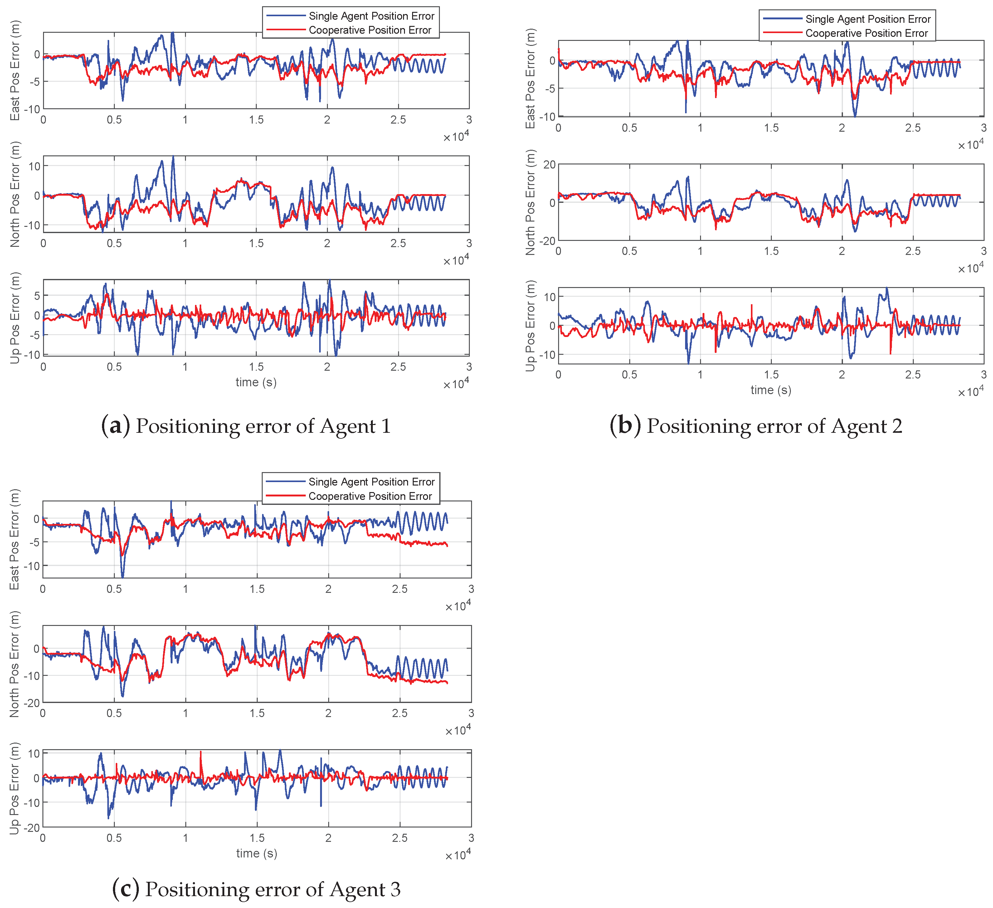
Similar to the simulation experiment, we estimate the position using two single-anchor positioning methods, and the components of positioning errors between the estimated position and the real position are shown in Figure 13. Additionally, the RMSE of the positioning results are shown in Table 6.
Although the correction effect of the eastward position and northward position is not as evident as the cooperative method in the simulation experiment, the vertical positioning error noticeably reduces when the agents are taken into consideration. Meanwhile, compared to the method without cooperation, the positioning error of the cooperative method when stationary is more stable.
The unexpected performance of the cooperative method may due to the error in the integrated navigation of the reference trajectories. Nevertheless, the positions estimated using the proposed single-anchor positioning method are much more accurate than those estimated by pure filtering.
7. Conclusions
This paper’s novel contribution is proposing a single-anchor cooperative positioning method for a multi-UAV system. The inertial measurements from the agents are optimized by the range measurements between the UAVs and the anchor. The process of Bayesian estimation is derived in detail with the model of sensors and the principle of inertial calculation. Simulation and real-world experiments are carried out, and the effectiveness of the method is proved. Although the estimated position cannot be completely consistent with the real one, it is enough in the case of insufficient sensor measurements. More experiments are required in future work to certify that the method is effective for more extensive ranges and agents.
Author Contributions
Conceptualization, J.Y.; Formal analysis, J.Y.; Funding acquisition, K.T.; Investigation, J.Y. and Y.G.; Methodology, J.Y.; Resources, Y.G.; Software, J.Y.; Supervision, Y.G. and K.T.; Visualization, Y.G.; Writing—original draft, J.Y.; Writing—review and editing, Y.G. and K.T. All authors have read and agreed to the published version of the manuscript.
Funding
This research is funded by the National Natural Science Foundation of China (62103424).
Data Availability Statement
Not applicable.
Conflicts of Interest
The authors declare that there are no conflict of interest regarding the publication of this paper.
Appendix A
The block matrices of state-transition matrix in (74) are calculated using the navigation parameters and the attitude, velocity, and position updated following the inertial calculation process, as shown below:
References
- Yu, X.; Li, Q.; Jorge, P.Q.; Tomi, W. Applications of UWB Networks and Positioning to Autonomous Robots and Industrial Systems. In Proceedings of the Mediterranean Conference on Embedded Computing (MECO), Budva, Montenegro, 7–10 June 2021. [Google Scholar]
- Wang, S.; Carmen, M.A.; Jorge, P.Q.; Zhou, Z.; Tomi, W. UWB-Based Localization for Multi-UAV Systems and Collaborative Heterogeneous Multi-Robot Systems. Procedia Comput. Sci. 2020, 175, 357–364. [Google Scholar]
- Perakis, H.; Gikas, V. Evaluation of Range Error Calibration Models for Indoor UWB Positioning Applications. In Proceedings of the 2018 International Conference on Indoor Positioning and Indoor Navigation (IPIN), Nantes, France, 24–27 September 2018. [Google Scholar]
- Li, M.; Zhu, H.; You, S.; Tang, C. UWB-Based Localization System Aided with Inertial Sensor for Underground Coal Mine Applications. IEEE Sensors J. 2020, 20, 6652–6669. [Google Scholar] [CrossRef]
- Pelletier, J.; O’Neill, B.; Leonard, J.; Freitag, L.; Gallimore, E. AUV-Assisted Diver Navigation. IEEE Robot. Autom. Lett. 2008, 7, 10208–10215. [Google Scholar] [CrossRef]
- Xu, C.; Xu, C.; Xing, W.; Herrera, V.E. Guided Trajectory Filtering for Challenging Long-Range AUV Navigation. IEEE Trans. Instrum. Meas. 2023, 72, 8502510. [Google Scholar] [CrossRef]
- Fang, X.; Wang, C.; Nguyen, T.; Xie, L. Graph Optimization Approach to Range-Based Localization. IEEE Trans. Syst. Man Cybern. Syst. 2018, 51, 6830–6841. [Google Scholar] [CrossRef]
- Lin, Z.; Fu, M.; Diao, Y. Distributed Self Localization for Relative Position Sensing Networks in 2D Space. IEEE Trans. Signal Process. 2015, 14, 3751–3761. [Google Scholar] [CrossRef]
- Li, X.; Luo, X.; Zhao, S. Globally Convergent Distributed Network Localization Using Locally Measured Bearings. IEEE Trans. Control Netw. Syst. 2020, 7, 245–253. [Google Scholar] [CrossRef]
- Poulose, A.; Emeršič, Ž.; Eyobu, O.S.; Han, D.S. An Accurate Indoor User Position Estimator For Multiple Anchor UWB Localization. In Proceedings of the International Conference on Information and Communication Technology Convergence (ICTC), Jeju, Republic of Korea, 21–23 October 2020. [Google Scholar]
- Lee, G.T.; Seo, S.B.; Jeon, W.S. Indoor Localization by Kalman Filter based Combining of UWB-Positioning and PDR. In Proceedings of the 2021 IEEE 18th Annual Consumer Communications & Networking Conference (CCNC), Las Vegas, NV, USA, 9–12 January 2021. [Google Scholar]
- Nguyen, T.M.; Zaini, A.H.; Wang, C.; Guo, K.; Xie, L. Robust Target-Relative Localization with Ultra-Wideband Ranging and Communication. In Proceedings of the IEEE International Conference on Robotics and Automation (ICRA), Brisbane, QLD, Australia, 21–25 May 2018. [Google Scholar]
- Wu, Y.; Pan, X. Velocity/Position Integration Formula Part I: Application to In-Flight Coarse Alignment. IEEE Trans. Aerosp. Electron. Syst. 2013, 49, 1006–1023. [Google Scholar] [CrossRef]
- Zheng, S.; Li, Z.; Liu, Y.; Zhang, H.; Zou, X. An Optimization-Based UWB-IMU Fusion Framework for UGV. IEEE Sensors J. 2022, 22, 4369–4377. [Google Scholar] [CrossRef]
- Cossette, C.C.; Shalaby, M.; Saussie, D.; Forbes, J.R.; Ny, J.L. Relative Position Estimation Between Two UWB Devices with IMUs. IEEE Robot. Autom. Lett. 2021, 6, 4313–4320. [Google Scholar] [CrossRef]
- Xu, Y.; Shen, T.; Chen, X.; Bu, L.; Feng, N. Predictive Adaptive Kalman Filter and Its Application to INS/UWB-integrated Human Localization with Missing UWB-based Measurements. Int. J. Autom. Comput. 2018, 16, 604–613. [Google Scholar] [CrossRef]
- Li, J.; Bi, Y.; Li, K.; Wang, K.; Lin, F.; Chen, B.M. Accurate 3D Localization for MAV Swarms by UWB and IMU Fusion. In Proceedings of the IEEE 14th International Conference on Control and Automation (ICCA), Anchorage, AK, USA, 12–15 June 2018. [Google Scholar]
- Feng, D.; Wang, C.; He, C.; Zhuang, Y.; Xia, X. Kalman-Filter-Based Integration of IMU and UWB for High-Accuracy Indoor Positioning and Navigation. IEEE Internet Things J. 2020, 7, 3133–3146. [Google Scholar] [CrossRef]
- Shalaby, M.; Cossette, C.C.; Ny, J.L.; Forbes, J.R. Cascaded Filtering Using the Sigma Point Transformation. IEEE Robot. Autom. Lett. 2021, 6, 4758–4765. [Google Scholar] [CrossRef]
- Pavlasek, N.; Walsh, A.; Forbes, J.R. Invariant Extended Kalman Filtering Using Two Position Receivers for Extended Pose Estimation. In Proceedings of the IEEE International Conference on Robotics and Automation (ICRA), Xi’an, China, 30 May–5 June 2021. [Google Scholar]
- Liu, Y.; Lian, B.; Zhou, T. Gaussian message passing-based cooperative localization with node selection scheme in wireless networks. Signal Process. 2019, 156, 166–176. [Google Scholar] [CrossRef]
- Shalaby, M.; Cossette, C.C.; Forbes, J.R.; Ny, J.L. Relative Position Estimation in Multi-Agent Systems Using Attitude-Coupled Range Measurements. IEEE Robot. Autom. Lett. 2021, 6, 4955–4961. [Google Scholar] [CrossRef]
- Zheng, S.; Li, Z.; Yin, Y.; Liu, Y.; Zhang, H.; Zheng, P.; Zou, X. Multi-robot relative positioning and orientation system based on UWB range and graph optimization. Measurement 2022, 195, 111068. [Google Scholar] [CrossRef]
- Großwindhager, B.; Stocker, M.; Rath, M.; Boano, C.A.; Römer, K. SnapLoc: An ultra-fast UWB-based indoor localization system for an unlimited number of tags. In Proceedings of the 18th International Conference on Information Processing in Sensor Networks, Montreal, QC, Canada, 16–18 April 2019; Volume 10, pp. 142–149. [Google Scholar]
- Wang, S.; Gu, D.; Chen, L.; Hu, H. Single Beacon based Localization with Constraints and Unknown Initial Poses. IEEE Trans. Ind. Electron. 2015, 63, 2229–2241. [Google Scholar] [CrossRef]
- Zhang, T.; Wang, Z.; Li, Y.; Tong, J. A Passive Acoustic Positioning Algorithm Based on Virtual Long Baseline Matrix Window. J. Navig. 2019, 72, 193–206. [Google Scholar] [CrossRef]
- Lu, L.; Li, Y.; Rizos, C. Virtual baseline method for Beidou attitude determination—An improved long-short baseline ambiguity resolution method. Adv. Space Res. 2013, 51, 1029–1034. [Google Scholar] [CrossRef]
- Reis, J.O.; Batista, P.T.M.; Oliveira, P.; Silvestre, C. Source Localization Based on Acoustic Single Direction Measurements. IEEE Trans. Aerosp. Electron. Syst. 2018, 54, 2837–2852. [Google Scholar] [CrossRef]
- Chen, L.; Cao, K.; Xie, L.; Li, X.; Feroskhan, M. 3-D Network Localization Using Angle Measurements and Reduced Communication. IEEE Trans. Signal Process. 2022, 70, 2402–2415. [Google Scholar] [CrossRef]
- Yuan, M.; Li, Y.; Li, Y.; Pang, S.; Zhang, J. A fast way of single-beacon localization for AUVs. Appl. Ocean Res. 2022, 119, 103037. [Google Scholar] [CrossRef]
- Cao, Y.; Yang, C.; Li, R.; Knoll, A.; Beltrame, G. Accurate position tracking with a single UWB anchor. In Proceedings of the IEEE International Conference on Robotics and Automation (ICRA), Paris, France, 31 May–31 August 2020. [Google Scholar]
- Yang, J.; Wu, M.; Cong, Y.; Guo, Y.; Zhou, X.; Tang, K. A Novel Single-beacon Positioning with Inertial Measurement Optimization. IEEE Robot. Autom. Lett. 2023. [Google Scholar] [CrossRef]
- IEEE Std 952-1997; IEEE Standard Specification Format Guide and Test Procedure for Single-Axis Interferometric Fiber Optic Gyros. The Institute of Electrical and Electronics Engineers, Inc.: New York, NY, USA, 1998.
- Groves, P.D. Principles of GNSS, Inertial, and Multisensor Integrated Navigation Systems. IEEE Aerosp. Electron. Syst. Mag. 2015, 30, 26–27. [Google Scholar] [CrossRef]
- El-Sheimy, N.; Hou, H.; Niu, X. Analysis and modeling of inertial sensors using Allan variance. IEEE Trans. Instrum. Meas. 2008, 57, 140–149. [Google Scholar] [CrossRef]
- Cano, J.; Chidami, S.; Ny, J.L. A Kalman Filter-Based Algorithm for Simultaneous Time Synchronization and Localization in UWB Networks. IEEE Robot. Autom. Lett. 2021, 6, 4955–4961. [Google Scholar]
- Mueller, M.W.; Hehn, M.; D’Andrea, R. A Computationally Efficient Motion Primitive for Quadrocopter Trajectory Generation. IEEE Trans. Robot. 2015, 31, 1294–1310. [Google Scholar] [CrossRef]
- Magnus, J.R.; Neudecker, H. Matrix Differential Calculus with Applications in Statistics and Econometrics; John Wiley & Sons: Hoboken, NJ, USA, 2019; pp. 87–110. [Google Scholar]
- Engelhardt, B. Introduction: Exponential family, conjugacy, and sufficiency. In STA561: Probabilistic Machine Learning; Princeton University: Princeton, NJ, USA, 2013; pp. 5–6. [Google Scholar]
Figure 1.
The block diagram of the classification of inertial errors.
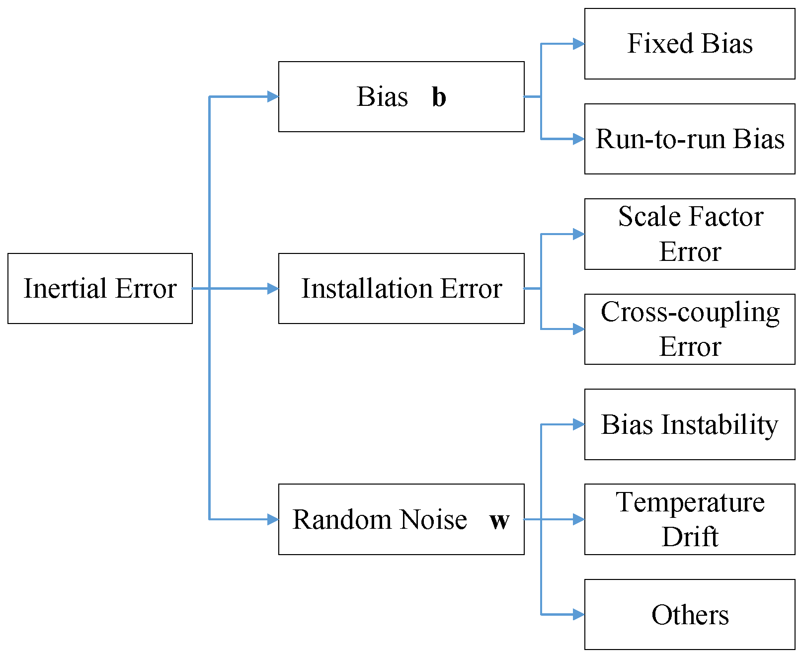
Figure 2.
Sensors and platform used in this paper.
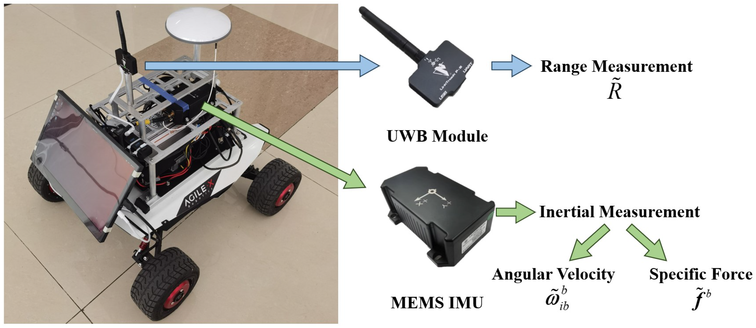
Figure 3.
The process of the optimization algorithm. The four blocks marked with red dashed boxes indicate the following subsections.
Figure 3.
The process of the optimization algorithm. The four blocks marked with red dashed boxes indicate the following subsections.
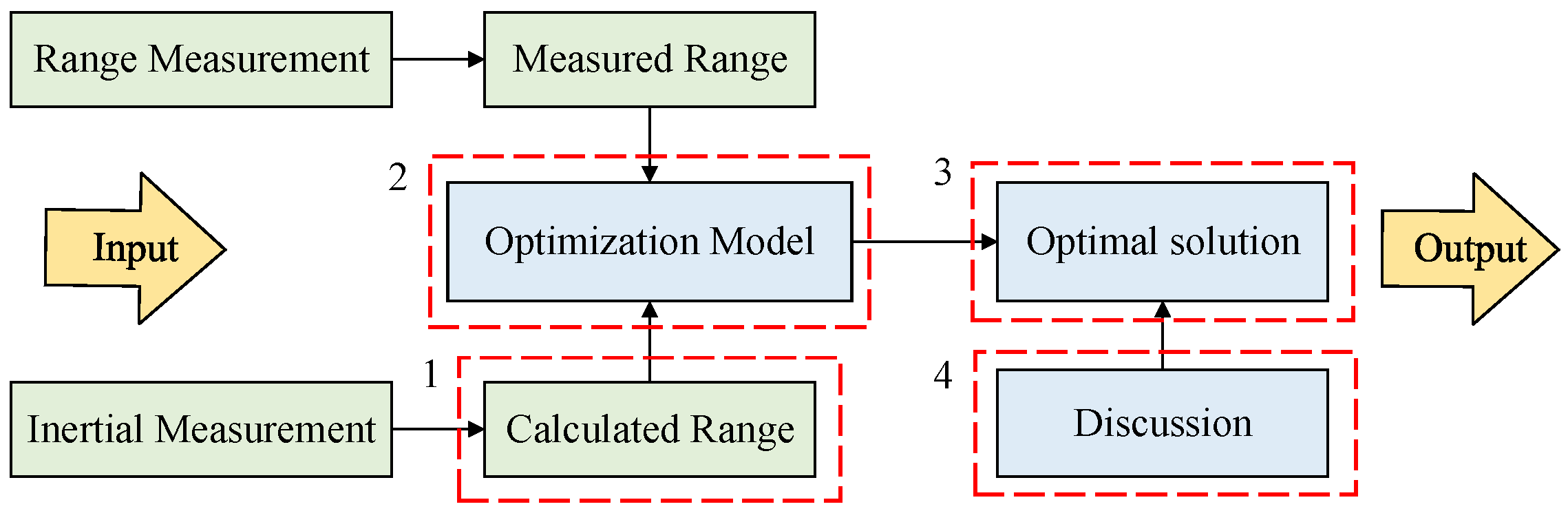
Figure 4.
A block diagram of the architecture of the single-anchor cooperative positioning method. The method includes two threads: optimization and filtering.
Figure 4.
A block diagram of the architecture of the single-anchor cooperative positioning method. The method includes two threads: optimization and filtering.

Figure 5.
Agent 1 and Agent 3 move anticlockwise in the horizontal plane along a square route for 7 circles and a half, as plotted by the arrow. Agent 2 and Agent 4 have a vertical takeoff and landing process, which move anticlockwise in a horizontal plane 100 m higher than Agent 1 and Agent 3.
Figure 5.
Agent 1 and Agent 3 move anticlockwise in the horizontal plane along a square route for 7 circles and a half, as plotted by the arrow. Agent 2 and Agent 4 have a vertical takeoff and landing process, which move anticlockwise in a horizontal plane 100 m higher than Agent 1 and Agent 3.
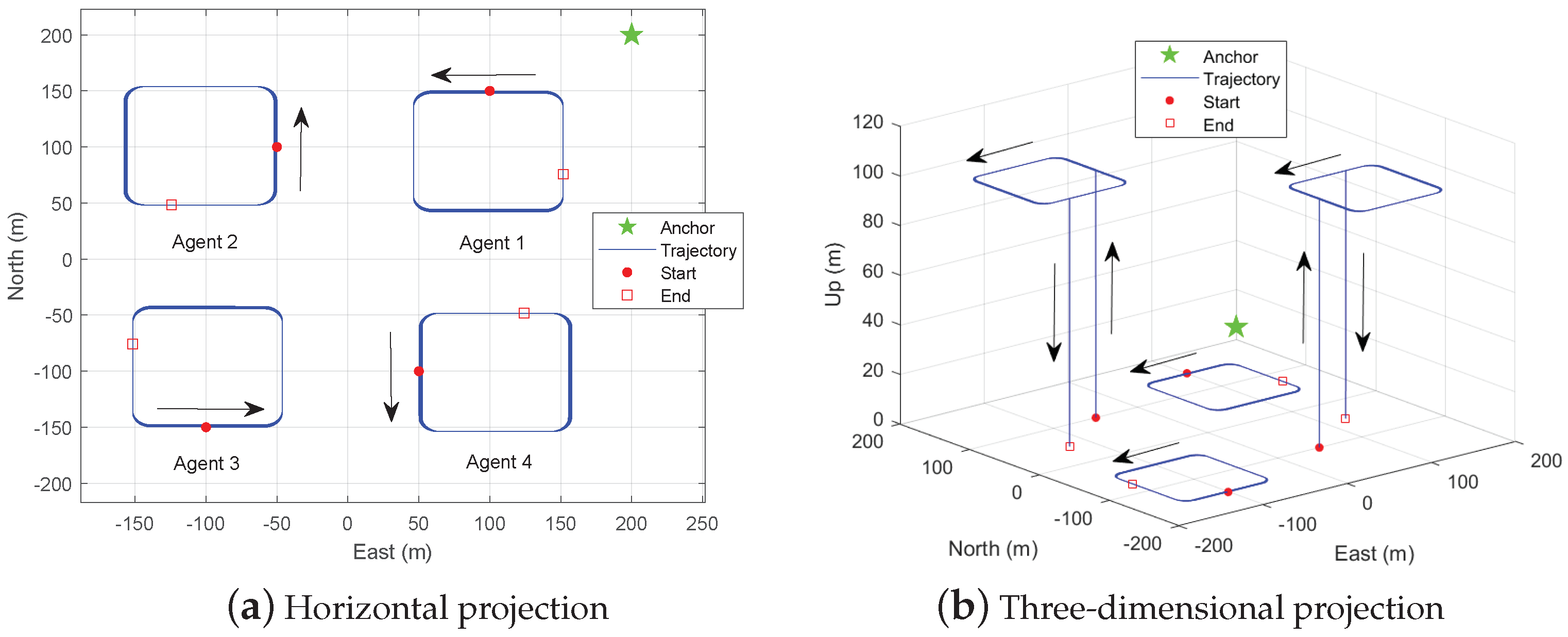
Figure 6.
The inertial measurements and unbiased truth−values in the simulation, which include angular velocity increments , , and and specific force incrementd , , and . x, y, and z indicate the direction of Right−Ahead−Up in the body frame.
Figure 6.
The inertial measurements and unbiased truth−values in the simulation, which include angular velocity increments , , and and specific force incrementd , , and . x, y, and z indicate the direction of Right−Ahead−Up in the body frame.
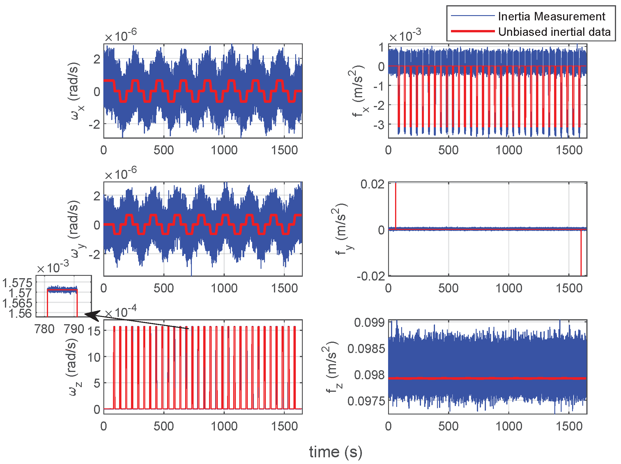
Figure 7.
The trajectories of pure optimization are shown in (a,b), and the trajectories of pure filtering are shown in (c,d). The trajectories in (a,b) have no height constraints, while the trajectories in (b,c) have height constraints.
Figure 7.
The trajectories of pure optimization are shown in (a,b), and the trajectories of pure filtering are shown in (c,d). The trajectories in (a,b) have no height constraints, while the trajectories in (b,c) have height constraints.
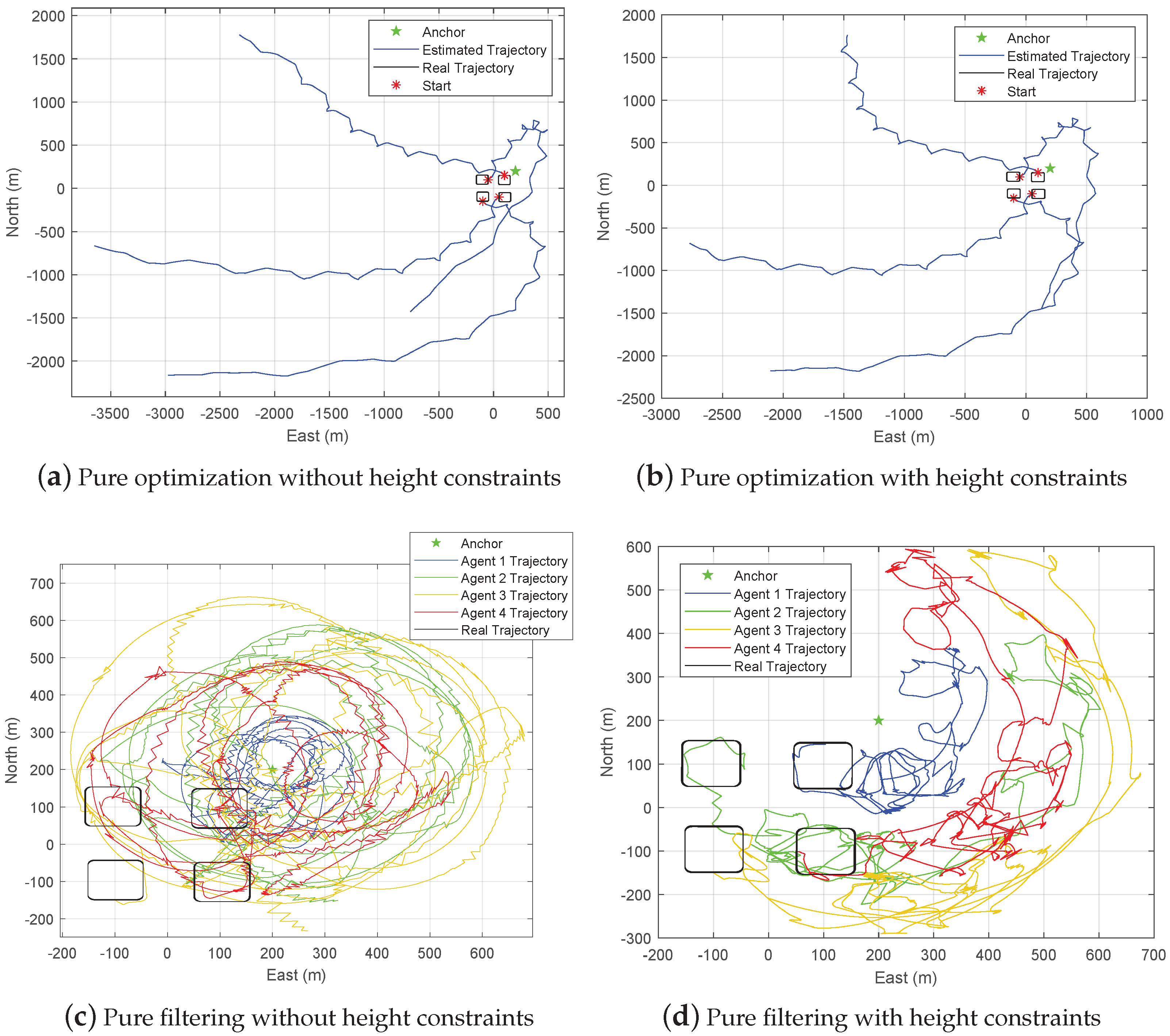
Figure 8.
The horizontal and three-dimensional projections of the trajectories solved using the single-anchor positioning method without the ranging measurements between the agents in simulation experiment.
Figure 8.
The horizontal and three-dimensional projections of the trajectories solved using the single-anchor positioning method without the ranging measurements between the agents in simulation experiment.
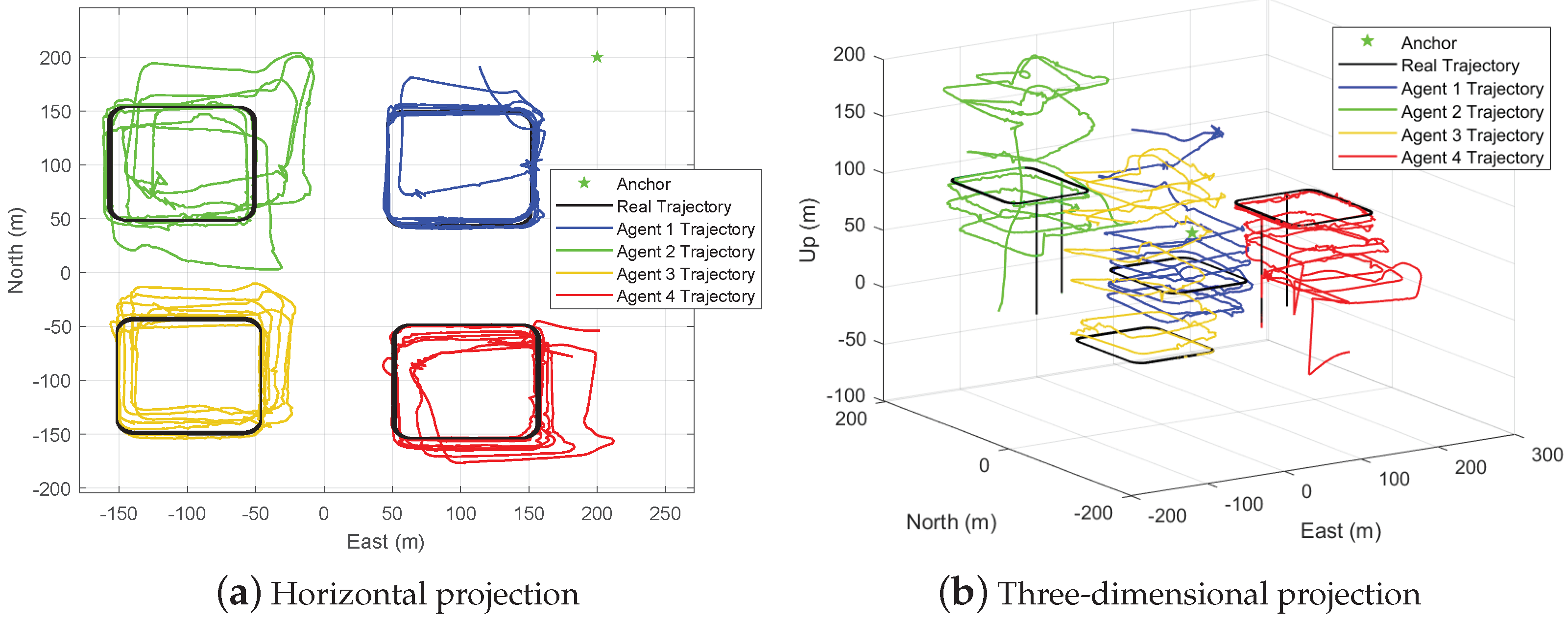
Figure 9.
The horizontal and three-dimensional projections of the trajectories solved using the single-anchor cooperative positioning method in simulation experiment.
Figure 9.
The horizontal and three-dimensional projections of the trajectories solved using the single-anchor cooperative positioning method in simulation experiment.

Figure 10.
The simulated positioning errors of two single−anchor positioning methods.

Figure 11.
The satellite imagery and sketch map of the real−world experiment environment. The anchor is placed as the green arrow in (a) and red star in (b). The starting points of three UGVs (or agents) are marked in (b), which are converted from navigation frame to a local coordinate frame.
Figure 11.
The satellite imagery and sketch map of the real−world experiment environment. The anchor is placed as the green arrow in (a) and red star in (b). The starting points of three UGVs (or agents) are marked in (b), which are converted from navigation frame to a local coordinate frame.
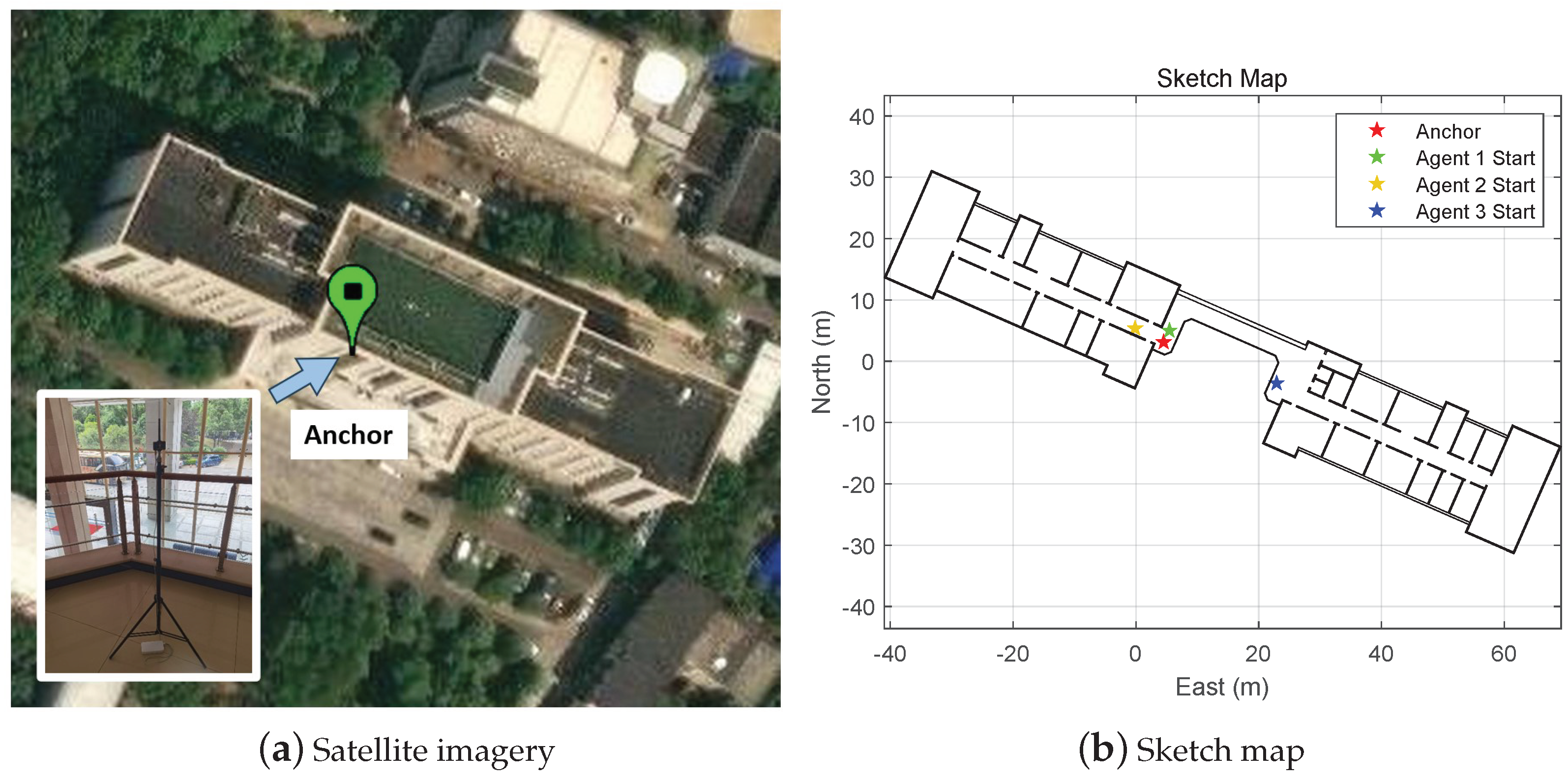
Figure 12.
The UGVs moving in the experimental environment. (a) is the picture of the vehicles and (b) indicates the reference trajectory of Agent 1. (c) shows the estimated trajectories by pure filtering.
Figure 12.
The UGVs moving in the experimental environment. (a) is the picture of the vehicles and (b) indicates the reference trajectory of Agent 1. (c) shows the estimated trajectories by pure filtering.
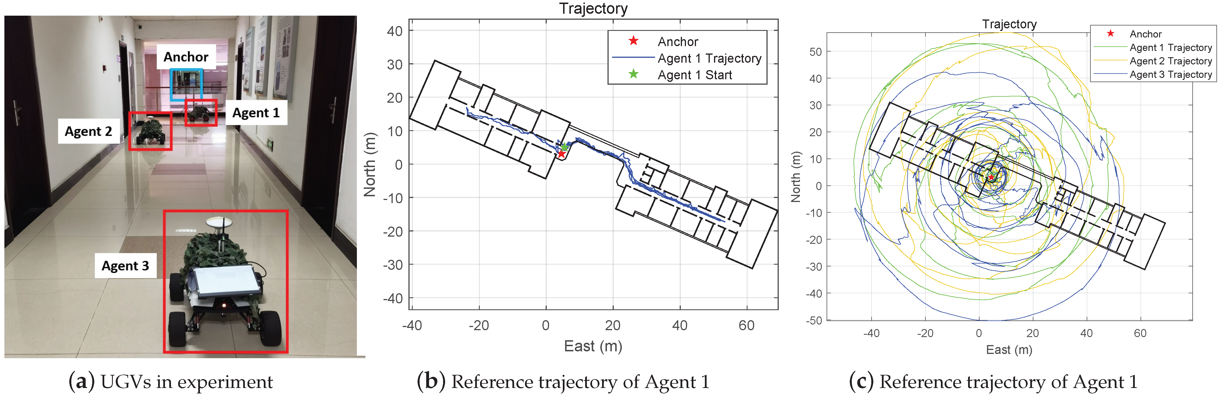
Figure 13.
The real−world positioning errors of two single−anchor positioning methods in the East, North, and Up directions in the navigation frame.
Figure 13.
The real−world positioning errors of two single−anchor positioning methods in the East, North, and Up directions in the navigation frame.

Table 1.
The number of conditional probabilities multiplied in Equation (37). There are four categories of conditional probabilities, including for the angular velocity of agent A, for the specific force of agent A, for the range between agent A and the single anchor, and for the range between agent A and agent B (measured by A).
| Conditional Probability | ||||
|---|---|---|---|---|
| Number | N | N | N |
Table 2.
Coordinates of the anchor and the starting points of the agents in the local coordinate frame.
Table 2.
Coordinates of the anchor and the starting points of the agents in the local coordinate frame.
| Point | Coordinate |
|---|---|
| Anchor | |
| Starting point of Agent 1 | |
| Starting point of Agent 2 | |
| Starting point of Agent 3 | |
| Starting point of Agent 4 |
Table 3.
Parameters used in the simulation experiment.
| Parameter | Value |
|---|---|
| Gyroscope constant bias | 0.2 |
| Gyroscope angular random walk | 0.02 |
| Accelerometer constant bias | 2 mg |
| Accelerometer velocity random walk | 0.2 |
| Inertial sensor frequency | 0.01 s |
| Ranging standard deviation | 0.1 m |
| Range sensor frequency | 0.1 s |
Table 4.
The RMSE of the positioning results of two single-anchor positioning methods in simulation experiment. For each agent and each method, there are the total RMSE and its components in the East, North, and Up directions, with the unit in meter.
Table 4.
The RMSE of the positioning results of two single-anchor positioning methods in simulation experiment. For each agent and each method, there are the total RMSE and its components in the East, North, and Up directions, with the unit in meter.
| Agent & Method | East | North | Up | Total |
|---|---|---|---|---|
| Single Agent, Agent 1 | 5.5288 | 17.8081 | 39.6870 | 43.8492 |
| Cooperative, Agent 1 | 1.6037 | 1.7913 | 9.2595 | 9.5665 |
| Single Agent, Agent 2 | 18.0673 | 20.4627 | 47.8726 | 55.1084 |
| Cooperative, Agent 2 | 3.5570 | 8.0210 | 14.0858 | 16.5952 |
| Single Agent, Agent 3 | 9.1513 | 11.6996 | 92.2450 | 93.4332 |
| Cooperative, Agent 3 | 5.2348 | 5.3550 | 22.1043 | 23.3384 |
| Single Agent, Agent 4 | 14.7703 | 11.5248 | 37.7707 | 42.1617 |
| Cooperative, Agent 4 | 5.2812 | 5.9927 | 17.0927 | 18.8671 |
Table 5.
Parameters used in the real-world experiment.
| Parameter | Value |
|---|---|
| Gyroscope constant bias | 1 |
| Gyroscope angular random walk | 0.1 |
| Accelerometer constant bias | 5 mg |
| Accelerometer velocity random walk | 0.5 |
| Inertial sensor frequency | 0.005 s |
| Ranging standard deviation | 0.1 m |
| Range sensor frequency | 0.02 s |
Table 6.
The RMSE of the positioning results of two single-anchor positioning methods in real-world experiment. For each agent and each method, there are the total RMSE and its components in the East, North, and Up directions, with the unit in meter.
Table 6.
The RMSE of the positioning results of two single-anchor positioning methods in real-world experiment. For each agent and each method, there are the total RMSE and its components in the East, North, and Up directions, with the unit in meter.
| Agent & Method | East | North | Up | Total |
|---|---|---|---|---|
| Single Agent, Agent 1 | 2.4677 | 4.7936 | 3.1790 | 6.2589 |
| Cooperative, Agent 1 | 2.4672 | 4.9743 | 1.3240 | 5.7082 |
| Single Agent, Agent 2 | 2.4240 | 4.7466 | 1.7510 | 6.4677 |
| Cooperative, Agent 2 | 2.2601 | 4.9688 | 3.6641 | 5.7326 |
| Single Agent, Agent 3 | 2.7217 | 5.6337 | 3.9202 | 7.3833 |
| Cooperative, Agent 3 | 3.1588 | 6.8185 | 1.0772 | 7.5915 |
Disclaimer/Publisher’s Note: The statements, opinions and data contained in all publications are solely those of the individual author(s) and contributor(s) and not of MDPI and/or the editor(s). MDPI and/or the editor(s) disclaim responsibility for any injury to people or property resulting from any ideas, methods, instructions or products referred to in the content. |
© 2023 by the authors. Licensee MDPI, Basel, Switzerland. This article is an open access article distributed under the terms and conditions of the Creative Commons Attribution (CC BY) license (https://creativecommons.org/licenses/by/4.0/).
Share and Cite
MDPI and ACS Style
Yang, J.; Guo, Y.; Tang, K. A Single-Anchor Cooperative Positioning Method Based on Optimized Inertial Measurement for UAVs. Drones 2023, 7, 577. https://doi.org/10.3390/drones7090577
AMA Style
Yang J, Guo Y, Tang K. A Single-Anchor Cooperative Positioning Method Based on Optimized Inertial Measurement for UAVs. Drones. 2023; 7(9):577. https://doi.org/10.3390/drones7090577
Chicago/Turabian StyleYang, Jinyi, Yan Guo, and Kanghua Tang. 2023. "A Single-Anchor Cooperative Positioning Method Based on Optimized Inertial Measurement for UAVs" Drones 7, no. 9: 577. https://doi.org/10.3390/drones7090577