
UASea: A Data Acquisition Toolbox for Improving Marine Habitat Mapping


1
Department of Marine Sciences, University of the Aegean, 81100 Mytilene, Greece
2
Department of Geography, University of the Aegean, 81100 Mytilene, Greece
*
Author to whom correspondence should be addressed.
Drones 2021, 5(3), 73; https://doi.org/10.3390/drones5030073
Submission received: 28 June 2021
/
Revised: 22 July 2021
/
Accepted: 30 July 2021
/
Published: 3 August 2021
(This article belongs to the Special Issue Ecological Applications of Drone-Based Remote Sensing)
Abstract
:Unmanned aerial systems (UAS) are widely used in the acquisition of high-resolution information in the marine environment. Although the potential applications of UAS in marine habitat mapping are constantly increasing, many limitations need to be overcome—most of which are related to the prevalent environmental conditions—to reach efficient UAS surveys. The knowledge of the UAS limitations in marine data acquisition and the examination of the optimal flight conditions led to the development of the UASea toolbox. This study presents the UASea, a data acquisition toolbox that is developed for efficient UAS surveys in the marine environment. The UASea uses weather forecast data (i.e., wind speed, cloud cover, precipitation probability, etc.) and adaptive thresholds in a ruleset that calculates the optimal flight times in a day for the acquisition of reliable marine imagery using UAS in a given day. The toolbox provides hourly positive and negative suggestions, based on optimal or non-optimal survey conditions in a day, calculated according to the ruleset calculations. We acquired UAS images in optimal and non-optimal conditions and estimated their quality using an image quality equation. The image quality estimates are based on the criteria of sunglint presence, sea surface texture, water turbidity, and image naturalness. The overall image quality estimates were highly correlated with the suggestions of the toolbox, with a correlation coefficient of −0.84. The validation showed that 40% of the toolbox suggestions were a positive match to the images with higher quality. Therefore, we propose the optimal flight times to acquire reliable and accurate UAS imagery in the coastal environment through the UASea. The UASea contributes to proper flight planning and efficient UAS surveys by providing valuable information for mapping, monitoring, and management of the marine environment, which can be used globally in research and marine applications.
1. Introduction
Habitat mapping is essential for marine spatial planning, management, and conservation of coastal marine habitats. Remotely sensed data combined with in-situ measurements are usually used for acquiring marine information. A plethora of remote sensing methods are available for marine habitat mapping; these methods differ as to the sensor, data resolution, spatial scale, expenses, repeatability, and data availability [1,2]. A variety of satellite sensors offer imagery from low (Landsat, Sentinel-2) to high resolutions (IKONOS, Quick Bird, Worldview) [3,4,5,6,7,8,9], while airborne sensors offer imagery with higher spatial resolutions at medium to large scales [10,11].
In recent years, the use of the UAS has been widespread in marine data acquisition in several coastal and marine applications [12,13,14,15,16,17]. The potential applications of the UAS in marine mapping and monitoring are constantly increasing, as they are an effective tool for acquiring high-resolution imagery [18,19,20,21] at a low cost and increased operational flexibility [22] in small to large areas [23]. The ability of the UAS to acquire sub-meter resolution imagery, which cannot be achieved using other remote sensing methods, fills the gap between satellite, airborne, and fieldwork data [16,22]. Thus, UAS allow the detection and accurate distinction of small marine features and the monitoring of habitat evolution [12,24].
However, the UAS surveys deal with many limitations related to the prevalent environmental conditions during data acquisition [25,26,27], which significantly reduce the possible acquisition times. These limitations have been analyzed extensively [28,29,30] while their effect on the quality of the UAS imagery has been reported in the recent literature [19,27,31,32]. UAS data acquisitions during non-optimal conditions lead to unreliable information and inaccurate results of marine habitat mapping [32].
The theoretical background of the parameters that affect the safety, accuracy, and reliability of the UAS surveys and aerial imagery quality in the marine environment has been presented through a UAS data acquisition protocol [33]. The UAS protocol consists of three main sections: (i) morphology of the study area, (ii) environmental conditions, and (iii) survey planning. The section on environmental conditions has been examined extensively, as the visible artifacts that are produced by them affect the sea surface and the water column, resulting in seabed visibility issues. The effect of the environmental conditions on high-resolution orthophoto-maps has been analyzed in an accuracy assessment study [32], identifying the sources of errors. The study proved that different environmental conditions result in different habitat coverages and classification accuracies. Although the optimal environmental conditions, flight paths [29], and flight altitude [31] for UAS data acquisition in the marine environment are well known, the detection of optimal acquisition times is still challenging.
In this study, we present the UASea, as a toolbox for the identification of the optimal flight times to acquire UAS data in the marine environment. The UASea calculates the optimal survey times for acquiring reliable UAS information in the coastal environment using a ruleset. The ruleset consists of forecast weather data (i.e., wind speed, wave height, precipitation prob., etc.) and adaptive thresholds that exclude the outlier values of each parameter. The result is an hourly basis prediction in a day, regarding the suggested or non-suggested UAS survey times. The toolbox suggestions were validated by the image quality estimations in both optimal and non-optimal acquisition times. The image quality estimates are derived by factors that mostly affect the UAS imagery, i.e., the sunglint, the sea surface texture, the water clarity, and image naturalness distortions.
The toolbox validation contributes to solving the crucial problem of the optimal acquisition times for efficient UAS surveys in the marine environment. This will lead to the informed selection of appropriate flight times and the collection of reliable information in the marine environment, avoiding unnecessary fieldwork hours and processing time, excessive use of the equipment, and a huge amount of inaccurate data. This study aims to propose the UASea toolbox as a data acquisition tool for efficient UAS surveys in the marine environment.
2. Materials and Methods
UASea is a toolbox that gives hourly positive or negative suggestions in a given day about the optimal or non-optimal UAS acquisition times to conduct a UAS survey in the coastal environment. The suggestions are derived using weather forecast data of weather variables and adaptive thresholds in a ruleset (Figure 1). To validate the performance of the UASea, we conducted UAS surveys in both optimal and non-optimal times. The acquired aerial imagery was then evaluated as to its quality. In this study, we used an image quality equation, which consists of four parameters that have been proved to significantly affect the quality and reliability of the remotely sensed imagery (i.e., sunglint presence, turbidity levels, sea-state conditions, image naturalness distortions). As the quality of the imagery is affected by the prevalent environmental conditions (e.g., wind speed, sunglint effect, waves) during data acquisition, the image quality estimations will provide more information on the permissible limits of each parameter.
2.1. UASea Toolbox
UASea toolbox is an interactive web application accessible through the internet from modern web browsers (https://uav.marine.aegean.gr/, accessed on 15 December 2020). It is designed using HTML and CSS scripts while JavaScript augments the user experience and user interactivity through mouse events (scroll, pan, click, etc.). It consists of a graphical user interface (GUI) component augmented by an app logic component (Figure 2), both framed and distributed by a web server for public access. GUI is a visual representation of various interactive visual components that allows users to interact with the UASea toolbox and is responsible for data input and output operations. Moreover, JavaScript is also responsible for app logic and calculations as the main core of the UASea toolbox. The app logic component utilizes user data input and asynchronously asks for weather forecast data in JSON format from the weather services, and based on the forecast values, suggests the optimal flight times suitable for marine applications. The results are presented in tabular format and additional figures for each forecast parameter, using Charts.js (Chart JS, https://www.chartjs.org/, accessed on 14 December 2020).
2.1.1. Weather Forecast Datasets
To identify the optimal flight times for marine mapping applications, the UASea toolbox uses short-range forecast data. In this context, we use (i) Dark Sky (DS) API (Dark Sky by Apple, https://darksky.net/, accessed on 10 May 2020) for two days of forecast data on an hourly basis and (ii) Open Weather Map (OWM) API (Open Weather Map, https://openweathermap.org/, accessed on 10 May 2020) five days forecast with three-hour step. Both services provide a limited free-of-charge usage of their APIs; DS allows up to 1000 free API calls per day, and OWM provides 60 calls per minute. The forecast data are provided in lightweight and easy-to-handle JavaScript Object Notation (JSON) file format on asynchronous API requests. DS API uses a great variety of data sources either globally, such as NOAA’s GFS model, German Meteorological Office’s ICON model, or regionally, such as NOAA’s NAMM available in North America, and aggregates them to provide a reliable and accurate forecast for any given location. OWM also uses several data sources such as NOAA GFS, ECMWF ERA, data from weather stations (companies, users, etc.), as well as satellite and weather radar data. Their numerical weather prediction (NWP) model was developed based on machine learning techniques.
2.1.2. Ruleset
The variables and their adaptive thresholds that constitute the toolbox ruleset are presented in Table 1. The parameters that have been proven to affect the quality of UAS imagery and flight safety have been used as variables in the ruleset. The suggested thresholds have been derived considering UAS protocols [25,26] and studies that have extensively analyzed the impact of the environmental conditions in marine applications [29,34,35,36], the UAS specifications [37], and fieldwork experience. The thresholds are used to exclude inconsistent and outlier values that may affect the quality of the acquired images as well as the safety of the survey and UAS pilot. Considering the above, the ruleset is designed in such a way that outlines the optimal weather conditions, suitable for reliable and accurate data acquisition, as well as for efficient short-range flight scheduling.
A set of mathematical rules based on Logical Conjunction and Set Theory was created using the mentioned ruleset. Every weather variable obtained by the weather APIs constitutes a distinct set, namely A for temperature, B for humidity, C for cloud coverage, D for the probability of precipitation, E for wind speed, F for the wave height, and G for sun elevation angle, while each one of the above sets is accompanied by an additional set (A’, B’, C’, D’, E’, F’, G’) that represents the adaptive thresholds. Optimal flight conditions necessitate the intersection between the former and the latter using Equation (1). The results of the equation imply two possible outcomes (0, 1), where 1 indicates optimal flight conditions while 0 stands for non-optimal flight conditions.
(A∩A′) ∧ (B∩B′) ∧ (C∩C′) ∧ (D∩D′) ∧ (E∩E′) ∧ (F∩F′) ∧ (G∩G′)
2.2. UASea Screens
GUI, along with its visual components, is depicted in Figure 3. Users may navigate to the map element by zooming in/out and panning to the desired location and selecting the study area by clicking the map (Figure 3a). After clicking the map, a leaflet marker is created that triggers the “Adjust Parameters” panel and button (Figure 3b). The Adjust Parameters panel consists of an HTML form in which users can adjust the parameters and their thresholds and select one of the available weather forecast data providers. By hitting the submit button, the parameter adjustment panel disappears, and the decision panel becomes available at the bottom of the screen. At the top of the decision panel (Figure 3c), there is a date menu that is used to address the range of the available forecast data, while on the bottom of the decision panel, the results of the UASea toolbox are presented in tabular format (Figure 3d). In the “Decisions” row, green indicates optimal weather conditions, while red stands for non-optimal weather conditions. Finally, a set of figures for each one of the weather parameters is also available through the figures panel (Figure 3e).
2.3. Validation
2.3.1. Image Quality Estimations (IQE)
The image quality equation (Equation (2)) is a combination of four variables (sunglint, waves, turbidity, image naturalness) that correspond to the conditions that affect the sea surface conditions, the water quality, and the image quality the most. As the images are acquired using an RGB sensor, we used RGB-based indices and statistics to quantify the effect of the parameters on the image quality. The processes were performed using R and Python packages. The image quality equation converts the values of each variable to an ascending number (from 1 to Ni, where (i) is the number of images) and calculates their summary per image. The summaries constitute the overall estimations of each image, where the lower value corresponds to the best quality image.
where x1 is the percentage of sunglint pixels, x2 the percentage of turbid pixels, x3 the variability of the image, and x4 the BRISQUE image quality estimation.
IQE = x1 + x2 + x3 + x4,
2.3.2. Sunglint Detection
A Brightness Index (BI) [38,39] was used for the sunglint detection (Equation (3)) to isolate the brighter pixels of the images that correspond to the sunglint pixels. To detect the brighter pixels of the image, we used the interquartile range (IQR) known as the Tukey fences method [40].
where Red is the digital number (DN) of the red channel, Green is the DN of the green channel, and Blue is the DN of the blue channel.
ΒΙ = (Red + Green + Blue)/3,
2.3.3. Turbidity Levels
The Normalized Difference Turbidity Index (NDTI) [41,42,43] was used to calculate the turbidity levels of the acquired imagery (Equation (4)). The values of the NDTI vary from −1 to 1, where higher values represent higher levels of turbidity. After the extraction of the NDTI images, an adaptive threshold was used for values ranging from 0.5 to 1 to isolate and calculate the number of high-turbid pixels in each image.
where, Red is the digital number (DN) of the red channel, and Green is the DN of the green channel.
NDTI = (Red − Green)/(Red + Green),
2.3.4. Image Texture
We used the grey-level co-occurrence matrix (GLCM) method as one of the most commonly used methods in image quality assessment [44,45,46] to measure the texture of the images [47]. A GLCM package in R was used to calculate the statistics: mean, variance, homogeneity, contrast, entropy, dissimilarity, second moment, and correlation of the red and green band of our images, derived from the grey-level co-occurrence matrices. A principal component analysis (PCA) was used to reduce the number of the texture bands where four PCs explained the 90% variability of the texture features. Statistical variability indicators (i.e., standard deviation, coefficient of variation) were used to examine the reliability of the results.
2.3.5. Image Naturalness
The Blind/Referenceless Image Spatial QUality Evaluator (BRISQUE) was used to provide an image quality score by comparing it to a default model based on natural-scene images as a distortion-independent measure of image quality assessment. The BRISQUE image quality score ranges from 0 to 100, where lower values refer to better quality [48]. The BRISQUE seems to perform well in measuring the naturalness of an image in cases where the exact type of image distortion is of no interest.
2.3.6. Correlation Analysis
We examined the correlation between the suggestions of the UASea toolbox per acquisition time to the image quality estimations, using the point biserial correlation method [49], as the one variable is dichotomous (yes/no) and the other is quantitative. The values of correlation coefficient vary from −1 to +1; positive values of r indicate the simultaneous increase or decrease of the variables, negative values of r indicate that when one variable increases, the other tends to decrease, while a zero value means that there is no linear relationship between the two variables. The results will allow us to measure the strength of the association between the two variables and to conclude on the reliability of the toolbox in the real world.
3. Results
3.1. UAS Surveys
Several surveys were conducted from May of 2020 to February of 2021 to examine the performance of the toolbox in seasonal conditions. The UAS surveys were conducted at both optimal and non-optimal times on each acquisition day, according to the suggestions of the toolbox, using a DJI Phantom 4 Pro system. The flight plan was created through Pix4Dcapture in a grid mission, and the settings were identical for each survey. The surveys were automated in a flight height of 70 m above ground, with a nadir viewing angle (90°), and the image overlap was set at 80%. The forecast weather data were acquired through the toolbox, while the local wind speed was measured using a handheld anemometer before each flight to verify that it matches the forecast values, and sky images were acquired to evaluate the cloud coverage.
The study area is a coastal area north of the town of Mytilene in Lesvos Island, Greece (Figure 4). The habitats of the seabed include an extended seagrass meadow of Posidonia Oceanica, one of the most significant seagrass species found only in the Mediterranean Sea. The morphology of the seabed also includes sandy areas and mixed types of algae in smaller depths, while the seabed depths range from 0.5 to 8 m. The surveyed area is easy to approach, close to a small harbor, and it belongs to the UAS free-flying zones.
We used a dataset of 20 surveys to validate the performance of the toolbox; 8 of the images were acquired in positive toolbox suggestions and 12 of them in negative toolbox suggestions. A sample of four acquisition dates is presented in Figure 5. Based on the toolbox suggestions, the first two surveys were conducted on 10 May 2020, at 4:00 p.m. and on 20 February 2021 at 2.00 p.m. at optimal acquisition times, while the surveys on 6 May 2020 at 12.00 p.m. and on 13 February 2021 at 12.00 p.m. were conducted at non-optimal acquisition times. The images acquired at optimal acquisition times are clear without sunglint presence; the first (10 May 2020) has a calm sea surface, while the second (20 February 2021) presents some wave wrinkles on the sea surface. The environmental conditions on these dates were within the adaptive thresholds of the toolbox. At both times, the wind speed was about 1 m/s, the sky was clear with a cloud cover lower than 25%, and sun elevation angles were between 25 to 45 degrees.
The images acquired at non-optimal acquisition times have a rough sea surface with sunglint presence that blurs the seabed information and prevents habitat distinction. At the two non-optimal acquisition times, the wind speed was 4 to 5 m/s, and the sky was partly cloudy. The negative results of the toolbox are due to the wind speed values, which are higher than the suggested 3 m/s, and the cloud cover, which was higher than 25%. Although the acquisition time of both dates was 12.00 p.m., the sun elevation angle on 6 May 2020 was higher than 45 degrees, while on 13 February 2021 it was lower than 45 degrees, as the sun is closer to the earth during the winter. This means that the thresholds of the sun elevation angle must be adapted according to the acquisition season to avoid the presence of sunglint on the images.
3.2. Validation Results
The calculations of the image quality estimates per variable and the overall estimates of the images are shown in Table 2. The x1, x2, x3, and x4 columns contain the calculated values of each variable, and the x1, x2, x3, and x4 sort columns, the ascending order of the values. The overall estimates are calculated by the summary of the variable estimates. The overall quality estimates vary from 12 to 61, where lower estimates correspond to higher image quality. The calculated sunglint percentages (x1) vary from 0.02% to 3.56%, the turbidity percentages (x2) from 0.02% to 2.77%, the variability of the image textures (x3) from 2.70 to 3.06, and the BRISQUE estimations (x4) from 3.34 to 35.67. Eight of the overall estimates are lower than the average value and correspond to the higher-quality images.
Most of the lower-quality images combine two to four high values of the variables. Considering the estimates of the lower-quality images per variable, it is observed that they almost equally affect the overall quality of the images. According to the toolbox forecasts, the higher-quality images were captured on wind speeds from 1 to 3 m/s, with cloud coverage from 0% to 25%, and acquisition times at morning and afternoon hours in the spring season while noon hours are included in the winter season. The lower-quality images were captured on wind speeds from 1 to 5 m/s, combined with high cloud coverages and acquisition times at morning to afternoon hours in the spring season and mostly noon hours in winter.
The higher-quality image (left) and the lower-quality image (right) as calculated by the image quality equation are shown in Figure 6. The higher-quality image was captured on 19 February 2021 at 12.00, and its quality estimation is 12, while the lower-quality image was acquired on 21 March 2020 at 13.00, and its quality estimation is 61. On the first date, the sunglint and turbidity percentages are very low, the texture of the image is smooth, and the BRISQUE estimation is 4.4, the fourth lower naturalness estimation of the dataset. The sea surface is calm, and the illumination of the seabed is sufficient for the distinction of marine habitats. On the second date, the sunglint covers 2.81% of the image, the sea surface texture is rough, and the BRISQUE estimation is 28.85, one of the higher image naturalness estimates of the dataset. The sea surface conditions prevent the clear visibility of the seabed, affecting the mapping of the habitats.
The biserial correlation showed a high association between the toolbox suggestions and the image quality estimations. The negative linear relationship between the two variables was significant as the coefficient r is 0.84 (df = 18, p < 0.05). The linear regression (Figure 7) shows that as the independent variable (overall estimates) increases, the dependent variable (toolbox suggestions) tends to decrease. In our study, this means that higher estimates (lower-quality images) correspond to the zero value of the toolbox suggestions (non-optimal acquisition times).
4. Discussion and Conclusions
The effect of UAS limitations on the quality of the acquired imagery and the accuracy of marine habitat mapping is widely known and reported in the literature [27,30,32,34]. Considering these limitations, we proposed the UASea as a toolbox for improving flight planning, the quality of the acquired data, and the mapping of marine habitats. The calculations of the UASea contribute to the detection of the optimal flight conditions for data acquisition in the marine environment. This is achieved by using the parameters that have been proved to significantly affect the quality of the acquired data, adapt thresholds on their values, and calculate the optimal survey times, influencing crucial decisions in the coastal environment. The challenges and limitations of UAS data acquisition in the marine environment are being overcome by the toolbox suggestions. The UASea is a valuable tool for efficient surveys that also contributes to the reduction of fieldwork costs, survey times, and time spent in the analysis and processing of unsatisfactory acquired data.
The dataset of images acquired in both optimal and non-optimal conditions enhanced the information on the conditions that affect the toolbox suggestions and the quality of the images. In total, 40% of the toolbox suggestions were positive, and their quality was higher than the average value, while 60% of the lower-quality images were acquired on time with high wind speeds and present high variability in their texture caused by the wavy sea surface. The 40% of the low-quality images were acquired at times with cloud coverages higher than 25% and/or sun angles lower than 25 or higher than 45 degrees, which may cause shading at the seabed, lack of adequate lighting, and sunglint presence on the sea surface [25,28,30,36,50]. Considering these results, the sea surface conditions, and the illumination of the seabed are the parameters that mostly affect the image quality.
The suggested acquisition times for sunglint avoidance while also achieving proper seabed lighting are early in the morning and late afternoon [11,34]. The higher-quality images are acquired at morning hours until 11.00 a.m. and at afternoon times from 4.00 p.m. to 7.00 p.m. at the spring–summer season, which corresponds to the suggested sun elevation angles (from 25 to 45 degrees). However, it is observed that the acquisition times differ in winter, where images acquired at noon hours have high image quality due to the sun elevation angles, which are lower during this season. This means that the suggested elevation angles may not be applicable in winter acquisition times. In general, the adaptive thresholds of the UASea ruleset seem to perform well in different seasons conditions and acquisition times. Allowing the user to change the suggested variable thresholds makes the toolbox more adaptable and its suggestions more accurate to each application.
It is important to mention that the UASea was initially developed for scientific purposes in the marine environment; however, it can be effectively used as a toolbox for implementing UAS surveys in different environments (e.g., urban, agricultural, inland waters, etc.) in environmental and ecological applications, such as detecting litter in the coastal zone [51,52] or floating marine litter [53], monitoring beach morphological changes [54,55], river habitat mapping [56], animal and wildlife monitoring [35,57], considering the respective weather parameters.
The correlation of the toolbox suggestions with the image quality estimations showed a high linear association between the two variables; most of the positive toolbox suggestions as optimal acquisition times match the images with the higher quality. The validation of the toolbox proved that UAS surveys on the suggested optimal acquisition times result in high-quality images. UAS as a widely used tool in high-resolution mapping at coastal areas, combined with the proposed toolbox, results in the acquisition of high-quality imagery. The significance of optimal UAS acquisition times advances the UASea as the optimum tool in overcoming the limitations that affect the quality of the acquired imagery. UASea is a user-friendly and promising toolbox that can be used globally for efficient mapping, monitoring, and management of the coastal environment, by researchers, engineers, environmentalists, NGOs for efficient mapping, monitoring, and management of the coastal environment, for ecological and environmental purposes, exploiting the existing capability of UAS in marine remote sensing.
Author Contributions
Conceptualization, M.D.; methodology, M.D.; software, M.B.; validation, M.D.; writing—original draft preparation, M.D.; writing—review and editing, M.D., M.B.; supervision, K.T. All authors have read and agreed to the published version of the manuscript.
Funding
This research received no external funding.
Data Availability Statement
The data that support the findings of this study are available from the corresponding author, Michaela Doukari, upon reasonable request.
Conflicts of Interest
The authors declare no conflict of interest.
References
- Hossain, M.S.; Bujang, J.S.; Zakaria, M.H.; Hashim, M. The Application of Remote Sensing to Seagrass Ecosystems: An Overview and Future Research Prospects. Int. J. Remote Sens. 2015, 36, 61–114. [Google Scholar] [CrossRef]
- Dat Pham, T.; Xia, J.; Thang Ha, N.; Tien Bui, D.; Nhu Le, N.; Tekeuchi, W. A Review of Remote Sensing Approaches for Monitoring Blue Carbon Ecosystems: Mangroves, Sea Grasses and Salt Marshes during 2010–2018. Sensors 2019, 19, 1933. [Google Scholar] [CrossRef] [PubMed] [Green Version]
- Topouzelis, K.; Spondylidis, S.C.; Papakonstantinou, A.; Soulakellis, N. The Use of Sentinel-2 Imagery for Seagrass Mapping: Kalloni Gulf (Lesvos Island, Greece) Case Study. In Proceedings of the Fourth International Conference on Remote Sensing and Geoinformation of the Environment (RSCy2016), Paphos, Cyprus, 12 August 2016; Themistocleous, K., Hadjimitsis, D.G., Michaelides, S., Papadavid, G., Eds.; International Society for Optics and Photonics SPIE: Bellingham, WA, USA, 2016; Volume 9688, p. 96881F. [Google Scholar]
- Topouzelis, K.; Makri, D.; Stoupas, N.; Papakonstantinou, A.; Katsanevakis, S. Seagrass Mapping in Greek Territorial Waters Using Landsat-8 Satellite Images. Int. J. Appl. Earth Obs. Geoinf. 2018, 67, 98–113. [Google Scholar] [CrossRef]
- Traganos, D.; Aggarwal, B.; Poursanidis, D.; Topouzelis, K.; Chrysoulakis, N.; Reinartz, P. Towards Global-Scale Seagrass Mapping and Monitoring Using Sentinel-2 on Google Earth Engine: The Case Study of the Aegean and Ionian Seas. Remote Sens. 2018, 10, 1227. [Google Scholar] [CrossRef] [Green Version]
- Hochberg, E.J.; Andréfouët, S.; Tyler, M.R. Sea Surface Correction of High Spatial Resolution Ikonos Images to Improve Bottom Mapping in Near-Shore Environments. IEEE Trans. Geosci. Remote Sens. 2003, 41, 1724–1729. [Google Scholar] [CrossRef]
- Pham, T.D.; Yokoya, N.; Bui, D.T.; Yoshino, K.; Friess, D.A. Remote Sensing Approaches for Monitoring Mangrove Species, Structure, and Biomass: Opportunities and Challenges. Remote Sens. 2019, 11, 230. [Google Scholar] [CrossRef] [Green Version]
- Tamondong, A.M.; Blanco, A.C.; Fortes, M.D.; Nadaoka, K. Mapping of Seagrass and Other Benthic Habitats in Bolinao, Pangasinan Using Worldview-2 Satellite Image. In Proceedings of the 2013 IEEE International Geoscience and Remote Sensing Symposium-IGARSS, Melbourne, Australia, 21–26 July 2013; pp. 1579–1582. [Google Scholar]
- Heenkenda, M.K.; Joyce, K.E.; Maier, S.W.; Bartolo, R. Mangrove Species Identification: Comparing WorldView-2 with Aerial Photographs. Remote Sens. 2014, 6, 6064–6088. [Google Scholar] [CrossRef] [Green Version]
- Klemas, V. Remote sensing of emergent and submerged wetlands: An overview. Int. J. Remote Sens. 2013, 34, 6286–6320. [Google Scholar] [CrossRef]
- Edmund, P.; Green, P.J.M.; Clark, A.J.E.; Clark, D. Remote Sensing Handbook for Tropical Coastal Management; Unesco Publishing: Paris, France, 2000; ISBN 9231037366. [Google Scholar]
- Ventura, D.; Bonifazi, A.; Gravina, M.F.; Ardizzone, G.D. Unmanned Aerial Systems (UASs) for Environmental Monitoring: A Review with Applications in Coastal Habitats, 2017. In Aerial Robots—Aerodynamics, Control and Applications; Mejia, O.D.L., Gomez, J.A.E., Eds.; IntechOpen: London, UK, 2017. [Google Scholar] [CrossRef] [Green Version]
- Sturdivant, E.J.; Lentz, E.E.; Thieler, E.R.; Farris, A.S.; Weber, K.M.; Remsen, D.P.; Miner, S.; Henderson, R.E. UAS-SfM for Coastal Research: Geomorphic Feature Extraction and Land Cover Classification from High-Resolution Elevation and Optical Imagery. Remote Sens. 2017, 9, 1020. [Google Scholar] [CrossRef] [Green Version]
- Husson, E.; Hagner, O.; Ecke, F. Unmanned Aircraft Systems Help to Map Aquatic Vegetation. Appl. Veg. Sci. 2014, 17, 567–577. [Google Scholar] [CrossRef]
- Ventura, D.; Bonifazi, A.; Gravina, M.F.; Belluscio, A.; Ardizzone, G. Mapping and Classification of Ecologically Sensitive Marine Habitats Using Unmanned Aerial Vehicle (UAV) Imagery and Object-Based Image Analysis (OBIA). Remote Sens. 2018, 10, 1331. [Google Scholar] [CrossRef] [Green Version]
- Casella, E.; Rovere, A.; Pedroncini, A.; Stark, C.P.; Casella, M.; Ferrari, M.; Firpo, M. Drones as Tools for Monitoring Beach Topography Changes in the Ligurian Sea (NW Mediterranean). Geo-Mar. Lett. 2016, 36, 151–163. [Google Scholar] [CrossRef]
- Papakonstantinou, A.; Doukari, M.; Stamatis, P.; Topouzelis, K. Coastal Management Using UAS and High-Resolution Satellite Images for Touristic Areas. Submitt. IGI Glob. J. 2017, 10, 54–72. [Google Scholar] [CrossRef] [Green Version]
- Whitehead, K.; Hugenholtz, C.H.; Myshak, S.; Brown, O.; LeClair, A.; Tamminga, A.; Barchyn, T.E.; Moorman, B.; Eaton, B. Remote Sensing of the Environment with Small Unmanned Aircraft Systems (UASs), Part 2: Scientific and Commercial Applications. J. Unmanned Veh. Syst. 2014, 02, 86–102. [Google Scholar] [CrossRef] [Green Version]
- Ridge, J.T.; Johnston, D.W. Unoccupied Aircraft Systems (UAS) for Marine Ecosystem Restoration. Front. Mar. Sci. 2020, 7, 1–13. [Google Scholar] [CrossRef]
- Donnarumma, L.; D’Argenio, A.; Sandulli, R.; Russo, G.F.; Chemello, R. Unmanned Aerial Vehicle Technology to Assess the State of Threatened Biogenic Formations: The Vermetid Reefs of Mediterranean Intertidal Rocky Coasts. Estuar. Coast. Shelf Sci. 2021, 251, 107228. [Google Scholar] [CrossRef]
- Monteiro, J.G.; Jiménez, J.L.; Gizzi, F.; Přikryl, P.; Lefcheck, J.S.; Santos, R.S.; Canning-Clode, J. Novel Approach to Enhance Coastal Habitat and Biotope Mapping with Drone Aerial Imagery Analysis. Sci. Rep. 2021, 11, 574. [Google Scholar] [CrossRef] [PubMed]
- Klemas, V.V. Coastal and Environmental Remote Sensing from Unmanned Aerial Vehicles: An Overview. J. Coast. Res. 2015, 315, 1260–1267. [Google Scholar] [CrossRef] [Green Version]
- Manfreda, S.; McCabe, M.F.; Miller, P.E.; Lucas, R.; Madrigal, V.P.; Mallinis, G.; Dor, E.B.; Helman, D.; Estes, L.; Ciraolo, G.; et al. On the Use of Unmanned Aerial Systems for Environmental Monitoring. Remote Sens. 2018, 10, 641. [Google Scholar] [CrossRef] [Green Version]
- Fallati, L.; Saponari, L.; Savini, A.; Marchese, F.; Corselli, C.; Galli, P. Multi-Temporal UAV Data and Object-Based Image Analysis (OBIA) for Estimation of Substrate Changes in a Post-Bleaching Scenario on a Maldivian Reef. Remote Sens. 2020, 12, 2093. [Google Scholar] [CrossRef]
- Finkbeiner, M.; Stevenson, B.; Seaman, R. Guidance for Benthic Habitat Mapping: An Aerial Photographic Approach; NOAA/National Ocean Service/Coastal Services Center: Charleston, SC, USA, 2001.
- Coggan, R.; Curtis, M.; Vize, S.; James, C.; Passchier, S.; Mitchell, A.; Smit, C.J.; Coggan, R.; Populus, J.; White, J.; et al. Review of Standards and Protocols for Seabed Habitats Mapping. Available online: https://www.researchgate.net/profile/Jonathan_White12/publication/269630850_Review_of_standards_and_protocols_for_seabed_habitat_mapping/links/55e06b7608ae2fac471b6de3/Review-of-standards-and-protocols-for-seabed-habitat-mapping.pdf (accessed on 5 January 2021).
- Nahirnick, N.K.; Reshitnyk, L.; Campbell, M.; Hessing-Lewis, M.; Costa, M.; Yakimishyn, J.; Lee, L. Mapping with Confidence; Delineating Seagrass Habitats Using Unoccupied Aerial Systems (UAS). Remote Sens. Ecol. Conserv. 2019, 5, 121–135. [Google Scholar] [CrossRef]
- Doukari, M.; Batsaris, M.; Papakonstantinou, A.; Topouzelis, K. A Protocol for Aerial Survey in Coastal Areas Using UAS. Remote Sens. 2019, 11, 1913. [Google Scholar] [CrossRef] [Green Version]
- Joyce, K.E.; Duce, S.; Leahy, S.M.; Leon, J.; Maier, S.W. Principles and Practice of Acquiring Drone-Based Image Data in Marine Environments. Mar. Freshw. Res. 2018, 70, 952–963. [Google Scholar] [CrossRef]
- Duffy, J.P.; Cunliffe, A.M.; DeBell, L.; Sandbrook, C.; Wich, S.A.; Shutler, J.D.; Myers-Smith, I.H.; Varela, M.R.; Anderson, K. Location, Location, Location: Considerations When Using Lightweight Drones in Challenging Environments. Remote Sens. Ecol. Conserv. 2018, 4, 7–19. [Google Scholar] [CrossRef]
- Ellis, S.L.; Taylor, M.L.; Schiele, M.; Letessier, T.B. Influence of Altitude on Tropical Marine Habitat Classification Using Imagery from Fixed-Wing, Water-Landing UAVs. Remote Sens. Ecol. Conserv. 2020, 2, 1–14. [Google Scholar] [CrossRef]
- Doukari, M.; Katsanevakis, S.; Soulakellis, N.; Topouzelis, K. The Effect of Environmental Conditions on the Quality of UAS Orthophoto-Maps in the Coastal Environment. ISPRS Int. J. Geo-Inf. 2021, 10, 18. [Google Scholar] [CrossRef]
- Doukari, M.; Topouzelis, K. UAS Data Acquisition Protocol for Marine Habitat Mapping: An Accuracy Assessment Study. In Proceedings of the International Archives of the Photogrammetry, Remote Sensing and Spatial Information Sciences—ISPRS Archives, Nice, France, 31 August–2 September 2020; Volume 43, pp. 1321–1326. [Google Scholar]
- Hodgson, A.; Kelly, N.; Peel, D. Unmanned Aerial Vehicles (UAVs) for Surveying Marine Fauna: A Dugong Case Study. PLoS ONE 2013, 8. [Google Scholar] [CrossRef] [PubMed] [Green Version]
- Casella, E.; Collin, A.; Harris, D.; Ferse, S.; Bejarano, S.; Parravicini, V.; Hench, J.L.; Rovere, A. Mapping Coral Reefs Using Consumer-Grade Drones and Structure from Motion Photogrammetry Techniques. Coral Reefs 2017, 36. [Google Scholar] [CrossRef]
- Mount, R. Acquisition of Through-Water Aerial Survey Images: Surface Effects and the Prediction of Sun Glitter and Subsurface Illumination. Photogramm. Eng. Remote Sens. 2005, 71, 1407–1415. [Google Scholar] [CrossRef]
- Leng, F.; Tan, C.M.; Pecht, M. Effect of Temperature on the Aging Rate of Li Ion Battery Operating above Room Temperature. Sci. Rep. 2015, 5. [Google Scholar] [CrossRef] [Green Version]
- Letu, H.; Nagao, T.M.; Nakajima, T.Y.; Matsumae, Y. Method for Validating Cloud Mask Obtained from Satellite Measurements Using Ground-Based Sky Camera. Appl. Opt. 2014, 53, 7523. [Google Scholar] [CrossRef] [PubMed]
- Yamashita, M.; Yoshimura, M. Development of Sky Conditions Observation Method Using Whole Sky Camera. J. Jpn. Soc. Photogramm. Remote Sens. 2008, 47, 50–59. [Google Scholar] [CrossRef] [Green Version]
- Tukey, J.W. Exploratory Data Analysis; Addison-Wesley Pub. Co.: Reading, MA, USA, 1977; ISBN 9780201076165. [Google Scholar]
- Elhag, M.; Gitas, I.; Othman, A.; Bahrawi, J.; Gikas, P. Assessment of Water Quality Parameters Using Temporal Remote Sensing Spectral Reflectance in Arid Environments, Saudi Arabia. Water 2019, 11, 556. [Google Scholar] [CrossRef] [Green Version]
- Lacaux, J.P.; Tourre, Y.M.; Vignolles, C.; Ndione, J.A.; Lafaye, M. Classification of Ponds from High-Spatial Resolution Remote Sensing: Application to Rift Valley Fever Epidemics in Senegal. Remote Sens. Environ. 2007, 106, 66–74. [Google Scholar] [CrossRef]
- Subramaniam, S.; Saxena, M. Automated algorithm for extraction of wetlands from IRS RESOURCESAT LISS III data. ISPRS-Int. Arch. Photogramm. Remote Sens. Spat. Inf. Sci. 2011, 3820, 193–198. [Google Scholar] [CrossRef] [Green Version]
- Hall-Beyer, M. GLCM Texture: A Tutorial v. 3.0. Arts Res. Publ. 2017, 75. [Google Scholar] [CrossRef]
- Gadkari, D. Image Quality Analysis Using GLCM. Master’s Thesis, University of Central Florida, Orlando, FL, USA, 2004. [Google Scholar]
- Albregtsen, F. Statistical Texture Measures Computed from Gray Level Coocurrence Matrices. Image Process. Lab. Dep. Inform. Univ. Oslo 2008, 5, 1–14. [Google Scholar]
- Pan, H.; Gao, P.; Zhou, H.; Ma, R.; Yang, J.; Zhang, X. Roughness Analysis of Sea Surface from Visible Images by Texture. IEEE Access 2020, 8, 46448–46458. [Google Scholar] [CrossRef]
- Mittal, A.; Moorthy, A.K.; Bovik, A.C. Blind/Referenceless Image Spatial Quality Evaluator. In Proceedings of the Conference Record—Asilomar Conference on Signals, Systems and Computers, Pacific Grove, CA, USA, 6–9 November 2011; pp. 723–727. [Google Scholar]
- Gupta, S. Das Point Biserial Correlation Coefficient and Its Generalization. Psychometrika 1960, 25, 393–408. [Google Scholar] [CrossRef]
- Anggoro, A.; Siregar, V.P.; Agus, S.B. The Effect of Sunglint on Benthic Habitats Mapping in Pari Island Using Worldview-2 Imagery. Procedia Environ. Sci. 2016, 33, 487–495. [Google Scholar] [CrossRef] [Green Version]
- Drones for Litter Mapping: An Inter-Operator Concordance Test in Marking Beached Items on Aerial Images|Elsevier Enhanced Reader. Available online: https://reader.elsevier.com/reader/sd/pii/S0025326X21005762?token=27E3C6D6EC8334E4925DAFFD101D1FB5F6B8B8885DAA7137B78CECA2299F6076DB3282F152F51498269281A268BA4061&originRegion=eu-west-1&originCreation=20210719135501 (accessed on 19 July 2021).
- Papakonstantinou, A.; Batsaris, M.; Spondylidis, S.; Topouzelis, K. A Citizen Science Unmanned Aerial System Data Acquisition Protocol and Deep Learning Techniques for the Automatic Detection and Mapping of Marine Litter Concentrations in the Coastal Zone. Drones 2021, 5, 6. [Google Scholar] [CrossRef]
- Topouzelis, K.; Papageorgiou, D.; Karagaitanakis, A.; Papakonstantinou, A.; Ballesteros, M.A. Remote Sensing of Sea Surface Artificial Floating Plastic Targets with Sentinel-2 and Unmanned Aerial Systems (Plastic Litter Project 2019). Remote Sens. 2020, 12, 2013. [Google Scholar] [CrossRef]
- Talavera, L.; del Río, L.; Benavente, J.; Barbero, L.; López-Ramírez, J.A. UAS as Tools for Rapid Detection of Storm-Induced Morphodynamic Changes at Camposoto Beach, SW Spain. Int. J. Remote Sens. 2018, 39, 5550–5567. [Google Scholar] [CrossRef]
- Topouzelis, K.; Papakonstantinou, A.; Doukari, M. Coastline Change Detection Using Unmanned Aerial Vehicles and Image Processing Techniques. Fresenius Environ. Bull. 2017, 26, 5564–5571. [Google Scholar]
- Whitehead, K.; Hugenholtz, C.H. Remote Sensing of the Environment with Small Unmanned Aircraft Systems (Uass), Part 1: A Review of Progress and Challenges. J. Unmanned Veh. Syst. 2014, 2, 69–85. [Google Scholar] [CrossRef]
- Linchant, J.; Lisein, J.; Semeki, J.; Lejeune, P.; Vermeulen, C. Are Unmanned Aircraft Systems (UASs) the Future of Wildlife Monitoring? A Review of Accomplishments and Challenges. Mammal Rev. 2015, 45, 239–252. [Google Scholar] [CrossRef]
Figure 1.
Data acquisition and processing pipeline: UASea toolbox for the identification of the optimal flight times. Validation of the UASea performance through an image quality equation.
Figure 1.
Data acquisition and processing pipeline: UASea toolbox for the identification of the optimal flight times. Validation of the UASea performance through an image quality equation.

Figure 2.
The architecture schema of the proposed toolbox.

Figure 3.
The UASea toolbox: (a) the main screen of the toolbox, (b) parameter adjustment panel, (c) date range of the weather forecast data, (d) decision panel and weather values result in tabular format, and (e) figures panel.
Figure 3.
The UASea toolbox: (a) the main screen of the toolbox, (b) parameter adjustment panel, (c) date range of the weather forecast data, (d) decision panel and weather values result in tabular format, and (e) figures panel.
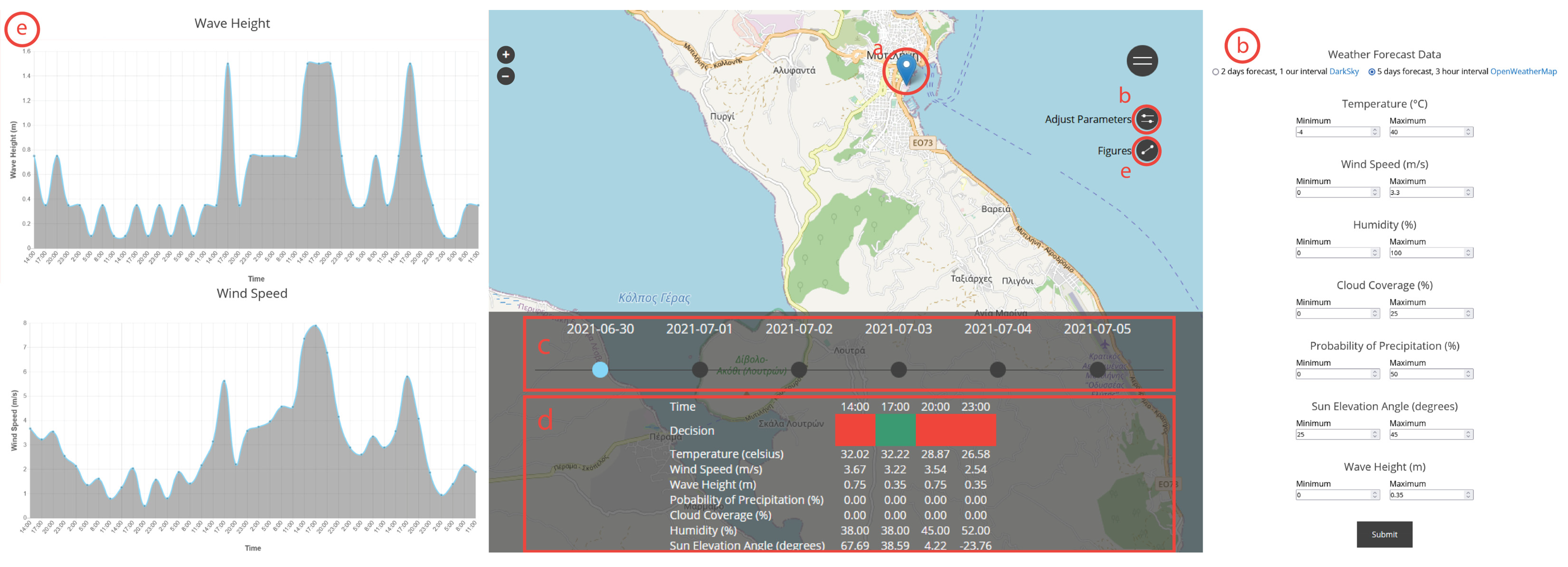
Figure 4.
Location map of the study area in Lesvos Island, Greece (left). The flight path of the UAS survey for data acquisition (right).
Figure 4.
Location map of the study area in Lesvos Island, Greece (left). The flight path of the UAS survey for data acquisition (right).

Figure 5.
Acquired images in optimal and non-optimal conditions on different dates, according to the toolbox. The two images on top were acquired at positive suggestions and the two at the bottom at negative suggestions.
Figure 5.
Acquired images in optimal and non-optimal conditions on different dates, according to the toolbox. The two images on top were acquired at positive suggestions and the two at the bottom at negative suggestions.
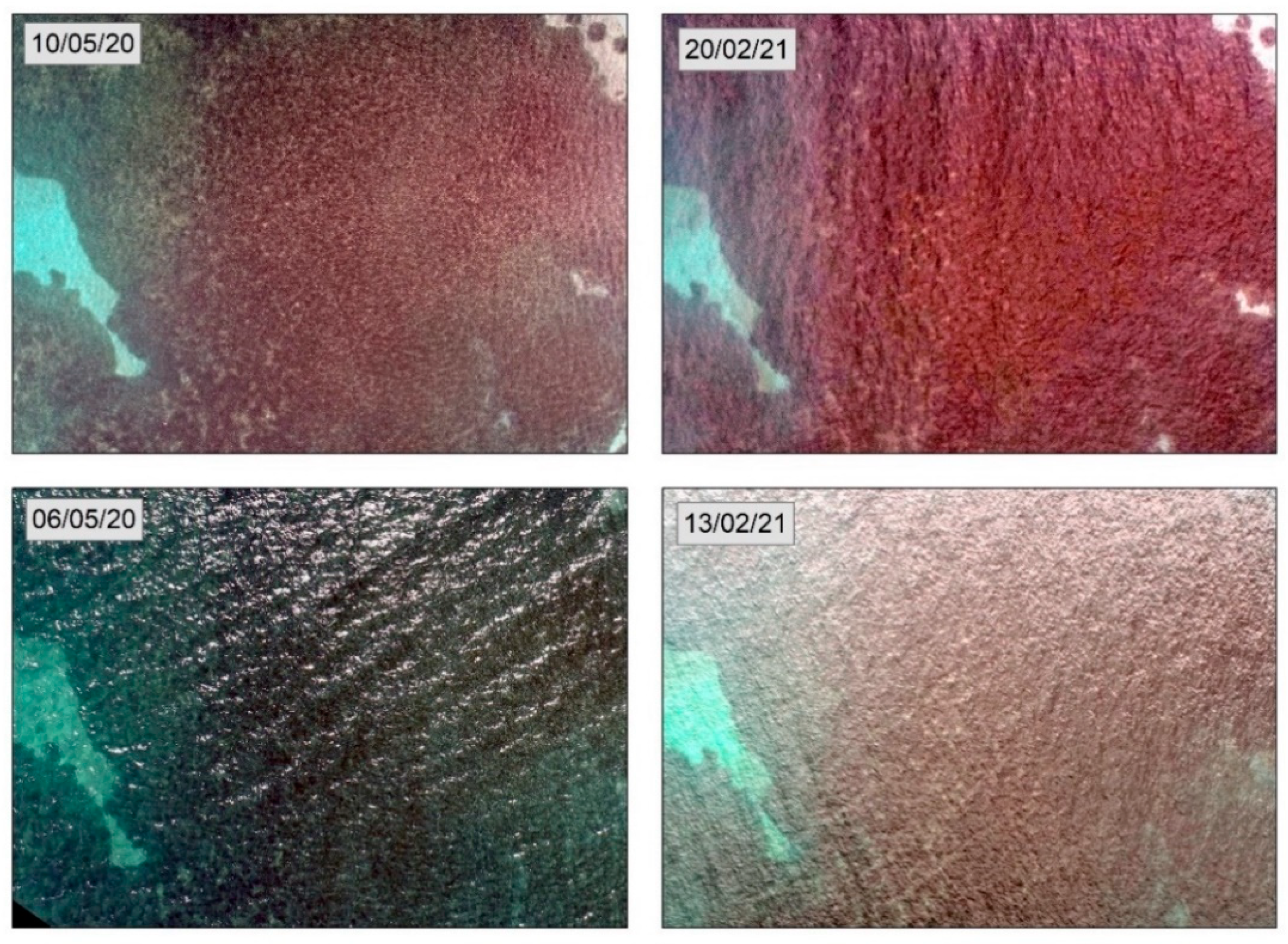
Figure 6.
The higher-quality image (left) with an overall estimation of 12 and the lower-quality image (right) with an overall estimation of 61, as calculated by the image quality equation.
Figure 6.
The higher-quality image (left) with an overall estimation of 12 and the lower-quality image (right) with an overall estimation of 61, as calculated by the image quality equation.
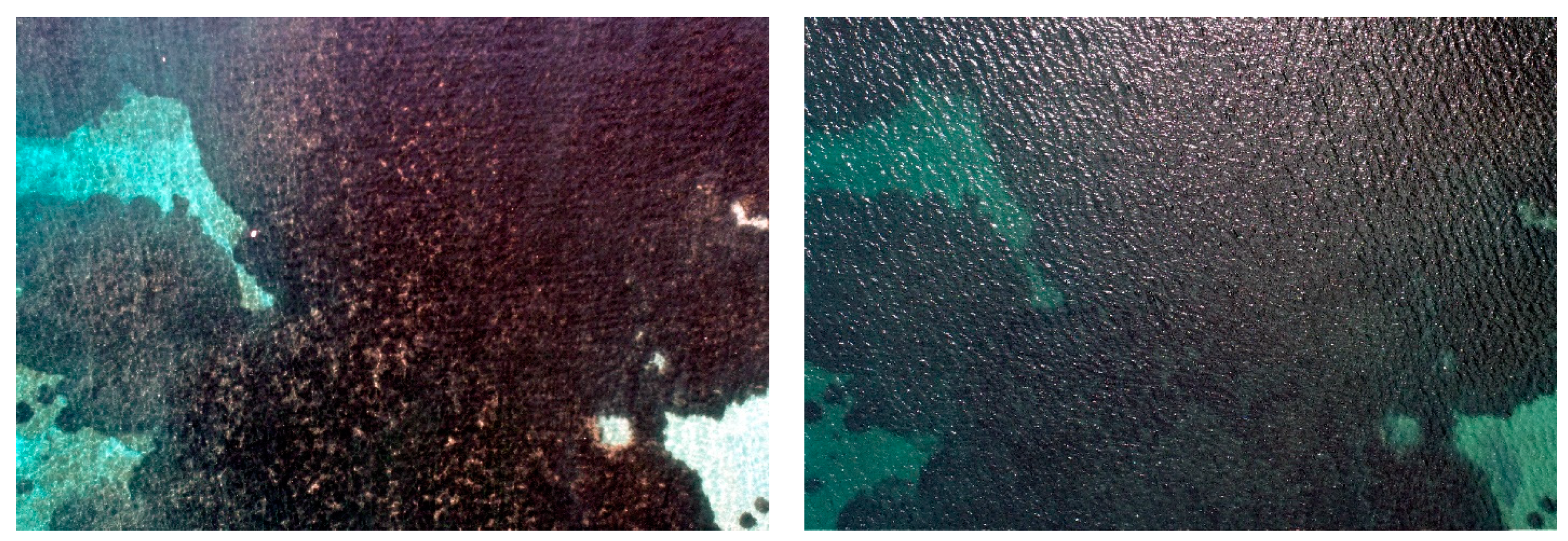
Figure 7.
Biserial correlation between the toolbox suggestions (0 for negative suggestion and 1 for positive suggestions) and the image quality estimates with a coefficient r 0.84. Higher estimates—lower-quality images correspond to the 0—negative suggestions of the toolbox.
Figure 7.
Biserial correlation between the toolbox suggestions (0 for negative suggestion and 1 for positive suggestions) and the image quality estimates with a coefficient r 0.84. Higher estimates—lower-quality images correspond to the 0—negative suggestions of the toolbox.


Table 1.
The variables and the adaptive thresholds of the ruleset for the calculation of the optimal flight times using the UASea.
Table 1.
The variables and the adaptive thresholds of the ruleset for the calculation of the optimal flight times using the UASea.
| Variables | Thresholds |
|---|---|
| Temperature (degrees Celsius) | −4–40 |
| Humidity (%) | 0–50 |
| Cloud cover (%) | 0–25 |
| Probability of precipitation (%) | 0–50 |
| Wind speed (m/s) | 0–3.3 |
| Wave height (m) | 0–0.35 |
| Sun elevation angle (degrees) | 25–45 |
Table 2.
The calculations of the image quality equation per variable and the overall quality estimates per image. The x1, x2, x3, and x4 columns contain the calculated values of each variable, while the x1, x2, x3, and x4 sort columns in the ascending order of the values. The overall estimates are calculated by the summary of the variable sorts. The lower the estimates, the higher the quality of the images.
| Image | x1 | x2 | x3 | x4 | x1 Sort | x2 Sort | x3 Sort | x4 Sort | Overall Estimates |
|---|---|---|---|---|---|---|---|---|---|
| 1 | 0.02 | 0.13 | 2.76 | 4.40 | 2 | 3 | 4 | 3 | 12 |
| 2 | 0.31 | 0.22 | 2.74 | 3.93 | 7 | 10 | 2 | 2 | 21 |
| 3 | 0.18 | 0.21 | 2.70 | 11.92 | 5 | 9 | 1 | 7 | 22 |
| 4 | 0.01 | 0.36 | 2.78 | 3.34 | 1 | 18 | 5 | 1 | 25 |
| 5 | 1.88 | 0.13 | 2.81 | 11.88 | 14 | 4 | 6 | 6 | 30 |
| 6 | 0.08 | 0.85 | 2.75 | 16.40 | 3 | 20 | 3 | 9 | 35 |
| 7 | 0.40 | 0.02 | 2.98 | 23.67 | 8 | 1 | 18 | 12 | 39 |
| 8 | 1.40 | 0.17 | 2.86 | 22.72 | 13 | 5 | 11 | 11 | 40 |
| 9 | 1.38 | 0.28 | 2.83 | 22.08 | 11 | 14 | 8 | 10 | 43 |
| 10 | 3.31 | 0.12 | 2.93 | 14.98 | 19 | 2 | 14 | 8 | 43 |
| 11 | 2.56 | 0.33 | 2.82 | 11.77 | 16 | 17 | 7 | 5 | 45 |
| 12 | 0.88 | 0.25 | 2.83 | 27.88 | 9 | 13 | 9 | 14 | 45 |
| 13 | 2.09 | 0.19 | 2.86 | 33.30 | 15 | 8 | 10 | 18 | 51 |
| 14 | 0.27 | 0.25 | 2.96 | 30.19 | 6 | 12 | 17 | 17 | 52 |
| 15 | 1.21 | 0.23 | 2.88 | 34.21 | 10 | 11 | 12 | 19 | 52 |
| 16 | 0.09 | 0.41 | 3.00 | 25.02 | 4 | 19 | 19 | 13 | 55 |
| 17 | 3.56 | 0.30 | 2.96 | 7.22 | 20 | 15 | 16 | 4 | 55 |
| 18 | 2.59 | 0.17 | 2.90 | 35.67 | 17 | 6 | 13 | 20 | 56 |
| 19 | 1.39 | 0.31 | 2.95 | 28.23 | 12 | 16 | 15 | 15 | 58 |
| 20 | 2.81 | 0.18 | 3.06 | 28.85 | 18 | 7 | 20 | 16 | 61 |
Publisher’s Note: MDPI stays neutral with regard to jurisdictional claims in published maps and institutional affiliations. |
© 2021 by the authors. Licensee MDPI, Basel, Switzerland. This article is an open access article distributed under the terms and conditions of the Creative Commons Attribution (CC BY) license (https://creativecommons.org/licenses/by/4.0/).
Share and Cite
MDPI and ACS Style
Doukari, M.; Batsaris, M.; Topouzelis, K. UASea: A Data Acquisition Toolbox for Improving Marine Habitat Mapping. Drones 2021, 5, 73. https://doi.org/10.3390/drones5030073
AMA Style
Doukari M, Batsaris M, Topouzelis K. UASea: A Data Acquisition Toolbox for Improving Marine Habitat Mapping. Drones. 2021; 5(3):73. https://doi.org/10.3390/drones5030073
Chicago/Turabian StyleDoukari, Michaela, Marios Batsaris, and Konstantinos Topouzelis. 2021. "UASea: A Data Acquisition Toolbox for Improving Marine Habitat Mapping" Drones 5, no. 3: 73. https://doi.org/10.3390/drones5030073