Article

Ground Control Point Distribution for Accurate Kilometre-Scale Topographic Mapping Using an RTK-GNSS Unmanned Aerial Vehicle and SfM Photogrammetry

1
School of Geographical and Earth Sciences, University of Glasgow, Glasgow G12 8QQ, UK
2
Department of Civil and Environmental Engineering, Brunel University London, Uxbridge UB8 3PH, UK
*
Author to whom correspondence should be addressed.
Drones 2020, 4(3), 55; https://doi.org/10.3390/drones4030055
Submission received: 10 July 2020 / Revised: 24 August 2020 / Accepted: 28 August 2020 / Published: 8 September 2020
(This article belongs to the Special Issue Drones in Geography)

Abstract

:
Unmanned Aerial Vehicles (UAVs) have revolutionised the availability of high resolution topographic data in many disciplines due to their relatively low-cost and ease of deployment. Consumer-grade Real Time Kinematic Global Navigation Satellite System (RTK-GNSS) equipped UAVs offer potential to reduce or eliminate ground control points (GCPs) from SfM photogrammetry surveys, removing time-consuming target deployment. Despite this, the removal of ground control can substantially reduce the georeferencing accuracy of SfM photogrammetry outputs. Here, a DJI Phantom 4 RTK UAV is deployed to survey a 2 × 0.5 km reach of the braided River Feshie, Scotland that has local channel-bar relief of c.1 m and median grain size c.60 mm. Five rectangular adjacent blocks were flown, with images collected at 20° from the nadir across a double grid, with strips flown in opposing directions to achieve locally convergent imagery geometry. Check point errors for seven scenarios with varying configurations of GCPs were tested. Results show that, contrary to some published Direct Georeferencing UAV investigations, GCPs are not essential for accurate kilometre-scale topographic modelling. Using no GCPs, 3300 independent spatially-distributed RTK-GNSS surveyed check points have mean z-axis error −0.010 m (RMSE = 0.066 m). Using 5 GCPs gave 0.016 m (RMSE = 0.072 m). Our check point results do not show vertical systematic errors, such as doming, using either 0 or 5 GCPs. However, acquiring spatially distributed independent check points to check for systematic errors is recommended. Our results imply that an RTK-GNSS UAV can produce acceptable errors with no ground control, alongside spatially distributed independent check points, demonstrating that the technique is versatile for rapid kilometre-scale topographic survey in a range of geomorphic environments.

1. Introduction

Topographic surveys of dynamic landforms, for scientific or management applications such as flow modelling [1,2], topographic change detection [3,4,5,6] and geomorphic unit mapping [7,8,9] typically cover areas of up to a few km2. In dynamic river environments, this scale demands using geomatics technologies that can address the threefold set of challenges posed by complex relief, inundated channels, and high rates of morphological change [1]. Digital photography and Unmanned Aerial Vehicle (UAV) hardware technologies [10,11,12] coupled with Global Navigation Satellite System (GNSS) placed ground control points (GCPs) and Structure-from-Motion with multiview stereo photogrammetry (SfM MVS; hereafter together referred to as SfM photogrammetry) [13] has become a widely established survey technique at this spatial scale [13,14,15,16,17,18]. The challenges for applying these technologies in dynamic environments compared to alternative techniques, such as static [19] and dynamic [20] terrestrial laser scanning, are: survey logistics including flight permissions, flight duration, weather and access for GCP placement [11,21,22,23,24]; imagery acquisition to mitigate structural errors [25,26]; and, postprocessing of point clouds to reconstruct accurate submerged topography [27,28] and classify vegetation [29]. The recent development of Direct Georeferencing (DG) of imagery captured by UAVs [30,31,32] potentially offers the opportunity to reduce the logistical challenge and time-consuming nature of GCP field operations [33]. Formally, Direct Georeferencing involves camera positioning using a UAV mounted GNSS antenna and no GCPs. GNSS observations are processed to provide the position of each image with centimetre-scale accuracy. In this paper we compare DG with a number of scenarios using different GCP configurations, using data from a Real Time Kinematic (RTK) GNSS equipped UAV. RTK positioning is achieved by an on-board GNSS receiver whose observed positions are adjusted using corrections that are transmitted from a radio that is part of a local GNSS base station whose position is well known. Little research or practical guidance exists for configuring ground control when working with RTK-GNSS UAVs in longitudinally extensive, corridor settings (e.g., river valleys, beaches) or to determine how using GCPs can influence the accuracy of topographic products.
UAVs are typically used in geomorphology applications to deploy a digital camera to acquire images for subsequent processing using SfM photogrammetry. To date, most UAV hardware setups include an onboard, standard, single-frequency GNSS receiver that is capable of geotagging digital images with a three-dimensional (3D) position calculated from code-based GNSS processing. This yields a positional accuracy of 5–10 metres. SfM photogrammetry uses highly redundant bundle adjustment to match features in multiple overlapping, offset images [34]. Geotagged images from a standard GNSS receiver speed up keypoint correspondence computations, but after SfM processing, the resulting sparse point cloud lacks accurate scale and orientation parameters because 3D point clouds are generated in a relative image-space coordinate system. The point clouds are subsequently transformed to an absolute coordinate system via a 3D linear similarity transformation based on GCPs with known object-space coordinates measured using ground survey. Metric data can then be extracted from the newly created point clouds. Recently an alternative georeferencing method for UAV imagery, Direct Georeferencing, has emerged whereby control is provided through the measurement of digital image location at exposure time to centimetre level accuracy [35] using a UAV mounted GNSS receiver that is capable of dual-frequency carrier and phase, and potentially multiconstellation, observations.
Direct Georeferencing of UAV acquired imagery can be achieved using one of four GNSS positioning and processing techniques [31]. First, from a local reference or base station, relative positioning using RTK corrections is achieved through a radio link between the base and UAV. Second, where a local reference is available but hardware for a radio link is not available, relative positioning can be achieved through the Post-Processed Kinematic (PPK) method. Both RTK and PPK GNSS processing can provide centimetre accuracy when baselines are short, i.e., less than a few kilometres [36]. Third, network RTK (NRTK) can be used to calculate relative position using a virtual reference station, with corrections from a network of GNSS reference stations received over the internet, via subscription to a service (e.g., HxGN SmartNet). Finally, Precise Point Positioning (PPP) offers an alternative relative positioning technique where highly accurate satellite orbit and clock parameters are fixed, for example using data from the International GNSS Service (IGS), and position is then estimated directly using dual-frequency carrier phase and code GNSS data. The advantage of PPP over the other techniques is that a local GNSS reference station is not needed nor does the flight area need to be served by NRTK correction.
Existing literature on geomorphological studies (Table 1) using UAVs capable of Direct Georeferencing, but sometimes supplemented with a small number of GCPs, primarily concerns experiments on urban areas or homogenous terrain <1 km2 in area. These types of sites allow testing of the UAV technology, but their relevance to heterogeneous natural environments and over larger, corridor areas needs to be assessed. This paper assesses the performance of an RTK-GNSS UAV in an upland river environment, so building upon the literature in terms of both spatial scale and shape and topographic variability. The three investigations published in 2017 in Table 1 [37,38,39] each used customised data processing and analysis and produced maximum check point elevation errors of the order of 1 m. Weber and Lerch [40] did not report independent elevation errors. Forlani et al. [32] and Taddia et al. [41] each assessed different GCP configurations. Forlani et al. [32] compared digital surface models (DSM) using Root Mean Squared Error (RMSE) statistics to determine the quality of SfM photogrammetry outputs based on different GCP scenarios. Taddia et al. [41] surveyed 2 km of coastline with a DJI Phantom 4 RTK and compared z-axis RMSE in PPK results. From the investigations in Table 1, assessments of the DG method suggest that: (i) DSMs georeferenced with no GCPs produce consistently higher z-axis RMSE than those with one or more GCPs [32]. For example, Forlani et al. [32] report RMSE with 12 GCPs of 0.026 m, 0.04 m for one GCP and 0.126 m with no GCPs; (ii) GCPs have limited influence on vertical errors [41], with z-axis RMSE of 0.022 m for DG with zero GCPs, decreasing only to 0.016 m when 21 GCPs were used; further, Taddia et al. [41] concluded that: (iii) a full oblique dataset is optimal for constraining z-axis errors, based on higher errors in both of the alternative image configurations that they used than in a full, double grid flight plan.
SfM derived geomorphological topographic datasets can have complex spatially distributed errors. These errors often result from systematic errors in the camera geometry. Such errors tend to arise when there is a weak image network geometry, usually arising from the flight plan geometry and design [11,43]. Additionally, errors may arise from inaccurate camera calibration arising from the estimation of photogrammetric parameters during the bundle adjustment phase of the SfM photogrammetry workflow. Such factors can then influence subsequent photogrammetric processing, resulting in a complex set of local optimization minima, in comparison to images captured in a highly convergent network [44]. Many previous studies have explored and have proposed mitigation for systematic errors, specifically doming, in geomorphic datasets via improved camera modelling [26,38]. Other approaches to reduce or eliminate systematic errors that have been considered include: the addition of oblique images in conjunction with a Nadiral datasets [41]; use of GCPs [45]; Direct Georeferencing techniques [42]; camera precalibration [46]; and, point of interest (POI) flight planning [45,47]. Of these approaches, POI is perhaps the most generally applicable but, for spatially extensive surveys along elongate corridors such as river valleys, double grids of convergent imagery (e.g., [41]), remains the most commonly used approach to acquiring images and warrants further error analysis. As Sanz-Ablanedo et al. [45] state, a limitation of the POI design is that the surveyed area cannot be more than four to five times the UAV flight height due to excessive convergence angles beyond this limit.
Many geomorphological studies have constraints of access over difficult terrain affecting GCP deployment and flight lines, and use is also often made of legacy images acquired using single or double grid flight plans. Hence, some of the error mitigation approaches proposed in the literature are unavailable in these situations. Consequently, the scope of our study is similar to Forlani et al. [32]’s investigation that tested the effect of different GCP numbers on imagery acquired using an RTK-GNSS UAV, although with DJI Phantom 4 RTK quadcopter UAV rather than a SenseFly eBee RTK fixed wing UAV. This DJI Phantom 4 RTK UAV was also used by Taddia et al. [41] but in PPK rather than the RTK mode that is used here. We consider the impact of the number and configuration of GCPs in an environment of similar scale and topographic complexity to that surveyed by Taddia et al. [41], which is significantly larger and more complex than the urban site used by Forlani et al. [32]. Specifically, the following research questions are addressed using an RTK approach to Direct Georeferencing: (i) are any GCPs needed when using an RTK-GNSS UAV? (ii) if GCPs are required, how many are needed? and, (iii) what is the optimal configuration for these GCPs? To address these questions, GCPs were distributed along and across a 2 × 0.5 km braided river reach to test different GCP configurations, using a consistent set of independent check points to assess accuracy. River and coastal surveys are typically longitudinally extensive and relatively narrow, as are a range of other settings (e.g., roads and railways) where the technology may be applied, thus requiring multiple UAV flights from different take off/landing positions to provide full coverage of the area of interest. This comprehensive analysis of the impact of the number of GCPs when using an RTK-GNSS UAV is used to provide guidance for corridor mapping (e.g., river valley) survey strategies in geomorphological environments and other settings of similar size and topography.

Study Area

Data were collected in Glen Feshie, United Kingdom in July 2019 from a 2 km length braided river reach (Figure 1). This reach has been the subject of multiple past topographic surveys that have tested new geomatics technologies for fluvial geomorphology applications and have developed new techniques to analyse surface sedimentology and sediment budgets [3,48,49,50]. The surveyed reach represents a dynamic section of the river where there are multiple wet channels at low flow and channel avulsion and switching occur during periods of high flow [51,52]. These channels are separated by compound bars with vegetation and bare gravels in the middle of the braidplain, as well as bank attached bars which exist intermittently on right and left banks. Bars range in length up to 500 m at times of low flow. Vegetated bars are colonised by a succession from grasses to shrubs, which form increasingly dense and large patches and tree saplings. The channel is incised into 0.1 to 2.0 m high fluvio-glacial terraces which have been observed to erode with time [53]. The reach has a large range in grain size with patches of material ranging from sand to boulders with an intermediate axis length of over 300 mm. Overall median grain size is 60 mm and the 95th percentile is 188 mm [54].

2. Materials and Methods

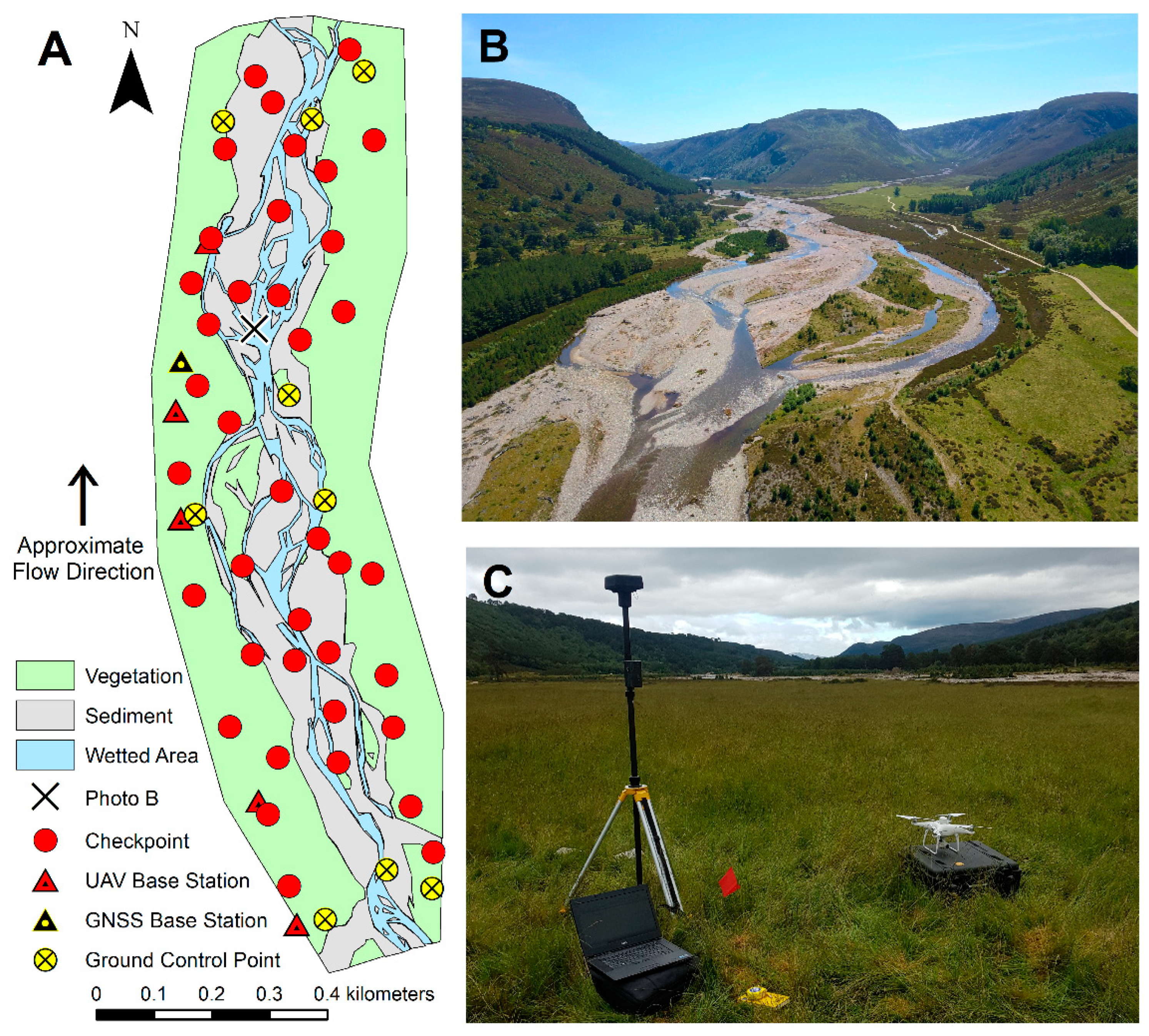
2.1. Field Data Acquisition

A Leica GS10 receiver was set up to occupy a previously established base station within the study area (Figure 1A; [50]). To provide coordinates for the UAV base stations, five semipermanent ground markers were installed along the 2 km length of the study site (Figure 1A). These five markers each provided a base station for one of five flight blocks that were needed to cover the study area and comply with visual line of sight requirements in accordance with the UK Civil Aviation Authority’s Drone Code. The location of each ground marker was observed in GNSS-static mode using a Leica AS10 GNSS Antenna for a period >2 h. These GNSS raw observations were postprocessed using Leica GeoOffice software relative to the already established study area base station. The position of each semiermanent ground marker was input as a known location into the UAV’s base station prior to the completion of each flight. The positional errors associated with the UAV base stations were submillimetre and are therefore be assumed to be negligible in the overall error analysis presented in this paper.
In addition to the benchmarks, 48 ground control targets were deployed across the study area (Figure 1A). Standard photogrammetric targets were used with dimensions of 0.6 × 0.6 m. Targets were subsequently divided into two groups. The first group (n = 9) were the ground control targets for different experiments. The second group (n = 39) provided a consistent set of check points to evaluate errors associated with each experiment. All targets were deployed on dry topography. Each target was observed with a Leica GS10 in GNSS-static mode for a period of five minutes. The AS10 antenna was mounted on a 2 m pole and positioned vertically over the central point of the yellow cross on each ground control target with a bipod. These raw GNSS static observations were postprocessed using the same method as for the ground markers that were used to position the UAV’s base station. These postprocessed point locations were then considered as the true locations of the targets’ centre points.
This investigation used a DJI Phantom 4 RTK UAV with an accompanying DJI base station (Figure 1C). This base station comprised a GNSS receiver and radio transmitter to send positional corrections to the UAV during flight. The product is marketed as consumer grade (<£5000). The hardware and software are relatively trivial to set up in comparison to professional survey grade GNSS or laser scanning equipment. Field setup required only two steps, taking no longer than ten minutes in total. The known coordinates of the ground marker benchmark were entered into the DJI base station, and radio communication was set up between this base and the UAV. Radio communication was maintained throughout the duration of each flight, allowing real-time positioning of the UAV relative to the known base location. This setup consequentially enables each digital image to be associated with an RTK corrected three-dimensional position.
The study area was flown by the UAV (see Table 2) within a 6-h period of overcast conditions to minimise variation in brightness during the survey. Flights were undertaken early in the morning when wind was negligible. The Phantom 4 RTK UAV controller contains an inbuilt electronic display which is programmed with bespoke DJI software to plan and execute UAV flights. For this survey, flights were planned to obtain images of sufficient quality to produce both a 2D orthomosaic image and a 3D Digital Elevation Model. Therefore, a 3D imaging flight plan option was chosen, which programs the UAV flight path to collect images across a double grid, whereby the UAV traverses the flight block in two orthogonal grid patterns. As per SfM photogrammetric best practice [55], and the findings of Taddia et al. [41], when acquiring images to generate 3D outputs the images were obtained at a 20 degree angle to the surface plane.

2.2. SfM Photogrammetry

Pix4D software was used for SfM photogrammetry. Although Pix4D’s interface is relatively automated, a series of parameters were set after importing the images to ensure the software recognised that the dataset was already georeferenced [57]. SfM photogrammetry processing parameters are summarised in Table 2. The DJI Phantom 4 RTK UAV uses the WGS84 coordinate system for flight navigation and to geotag digital images. The WGS84 coordinates were transformed to ETRS89 as this is standard across Europe and is used in the UK as the datum for all Ordnance Survey GNSS positioning [58]. In addition to the image data, RTK-GNSS point data relating to target centre point locations were input into the project, also in ETRS89.
The three-stage SfM photogrammetry processing workflow in Pix4D was used. Stage 1 involved matching keypoints from the UAV image data, and then automatic aerial triangulation and bundle block adjustment to create a 3-D point cloud of the study reach. At this stage, the images were georeferenced by the UAV RTK-GNSS data alone, and all target information is considered as check points. Check points indicate how well the point cloud was georeferenced, and show relative x, y and z errors for a given georeferencing scenario. A consistent set of 39 check points were identified and the remaining 9 targets were alternated between being marked as ground control points or check points depending on the experiment, if a target (n = 9) was marked as a check point it was then omitted from the error analysis so the comparison was consistent. The experiments presented here were all completed at this stage in the processing chain and are therefore related to the georeferencing of the point cloud dataset. Stages 2 and 3 of processing, which involve point cloud densification using multiview stereo and the generation of Digital Surface Model (DSM) and orthoimage products, were undertaken for the 0 and 5 GCP scenarios to further analyse and illustrate the outputs.

2.3. Ground Control Point Test Scenarios

The aim of the test scenarios was to investigate how the accuracy of the SfM point cloud changed as a result of using different numbers and configurations of ground control points. Seven experiments were conducted, ranging from zero to six GCPs, in varying configurations (Figure 2). The specific configurations were designed based on where the current literature suggests that adding ground control has a significant influence on minimising errors in the resultant DSM, for example at the edges of the survey extent [11]. The error analysis focused upon vertical rather than horizontal accuracy as elevation is harder to quantify correctly than horizontal position using GNSS technologies because errors are lower when satellites triangulate a horizontal point on the Earth’s surface than a vertical point some distance above the surface [59]. Additionally, in fluvial applications the error in the vertical dimension is comparatively more significant than horizontal errors because the lateral relief of the active channel belt rarely exceeds a few metres and is often less than this.

2.4. Validation: RTK-GNSS Water Edge Check Points

To assess for systematic vertical errors across the study area, a further ground survey dataset was acquired. An RTK-GNSS point data survey was undertaken along the Water Edge (WE) of all channels (anabranches) of the river. This dataset contained 3300 points that were distributed along the full length and width of the study area. These data were used to assess vertical error across a greater geographic coverage and at a greater density than the 39 check points. Point values from the WE dataset were compared to point elevations from the DSM outputs for both the 0 and 5 GCP scenarios (Figure 2A,F). Summary error statistics were calculated, and the spatial distribution of errors were mapped.

3. Results

3.1. Ground Control Point Analysis

Errors from the consistent set of 39 check points are summarised in Table 3, and z-axis errors are displayed in Figure 3. Mean Absolute Errors (MAEs) for the scenario with zero ground control points were 0.016 m, 0.020 m and 0.056 m, for the x, y and z axes, respectively. Standard Deviations (SDs) for this scenario were also smaller in magnitude for the planimetric axes (SDx = 0.022 m, SDy = 0.024 m) than the vertical axis (SDz = 0.070 m). The RMSEs also followed this trend, with values of 0.023 m, 0.024 m and 0.073 for the x, y and z axes, respectively. Overall, these summary statistics indicate that topography was reconstructed with minimal bias and relatively low variability; the higher errors for elevation are typical for a survey of the Earth’s surface.
The addition of ground control points had limited impact on the MAE in all three axes, with ≤0.007 m discrepancy between the 0 GCP scenario and all other scenarios, for all three axes. The x-axis had the highest range in MAE of 0.007 m, compared to 0.002 m and 0.003 m for the y- and z-axes, respectively. Standard deviations were very similar across all scenarios with a maximum range in SD of 3 mm for the z-axis and ≤2 mm range in SD for both the x- and y-axes. RMSE is again broadly consistent across all scenarios for all three axes with a range of 0.010, 0.003 and 0.005 m for the x, y and z axes, respectively. Six out of seven scenarios have a modal error <0.05 m. This consistency, despite a variation in GCP number and configuration, highlights that errors were constrained when using a DG UAV without any GCPs. This is supported by results for all test scenarios displaying very similar results to the 0 GCP scenario across the four error statistics.
Z-axis absolute errors for scenarios with GCPs ranged from 0.00 to 0.14 m (Figure 3), with all histograms showing a positive skew. The histogram for 0 GCPs (Figure 3A), shows a bimodal distribution which is a result of an area where there were consistently higher errors (area a-a’, Figure 3A). This bimodality is also observed in some of the other scenarios which show a larger range in spatial errors but is most distinct for scenarios with 0, 2, 4 and 6 GCPs. This area (a-a’) of higher errors is also observed when less than three GCPs were used. This spatial clustering of errors is less obvious for scenarios with 3 and 5 GCPs but was still present for the 4 and 6 GCPs scenarios.
The spatial patterns of odd (3,5) and even (4,6) GCPs suggest that having a control point in the centre of the study area, as well as others at the edges, is important to reduce spatially concentrated relatively high vertical errors. Further analysis was carried out on an additional 3300 independent check points to test whether the higher errors in region a-a’ were systematic.

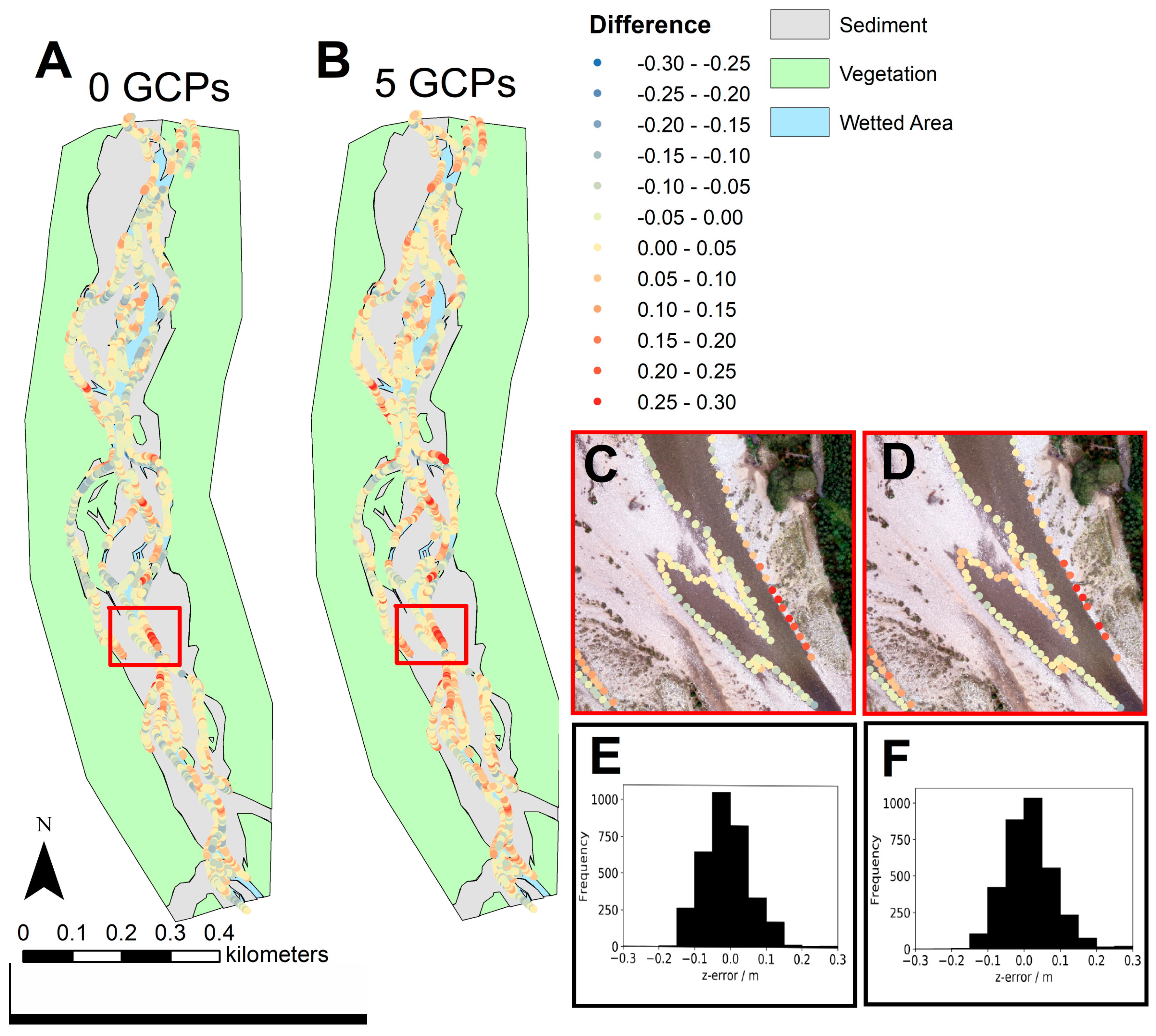
3.2. Check Point Validation

Summary error statistics for the 3300 WE check points (Table 4) have very similar magnitudes to those for the target check point analysis (Table 3). ME, MAE, RMSE and SDE all have z-axis errors within 7 mm of those from the 39 check points. Mean error differences are larger (0.028 and 0.036 m; Table 4) due to the signs of errors in the check point and water edge surveys being different in both scenarios.
The spatial distribution of errors (Figure 4A,B) is similar for the 0 and 5 GCP scenarios. The modelled DSM slightly over and under represents errors in the same locations irrespective of the number of GCPS used. As shown by the ME statistics in Table 4, the modelled DSM for 0 GCPs slightly underestimates elevation and the DSM for five GCPs slightly overestimates elevation. The histograms of errors (Figure 4E,F) also demonstrate this difference in the direction of each DSM’s vertical error.
In contrast to the higher errors for the check points in area a-a’ (Figure 3), Figure 4 does not show any spatially consistent areas of higher errors. Considering the spatial extent of the dataset, the spatial pattern of errors in Figure 4 indicates that systematic errors, such as a doming effect, are not evident within the SfM DSM outputs. Higher MAEs are observed in areas where there is relatively steep (near vertical or vertical) slope and the water edge is positioned on this slope. The nature of the WE survey therefore introduces local features in the data that are associated with the nature of the check point locations and local terrain gradient rather than reflecting systematic DSM errors. Errors are typically closer to 0 when water edge points are on gently sloping bars rather than steep banks (Figure 4C–D).

4. Discussion

4.1. Ground Control

Based on the results of Forlani et al. [32], it was hypothesised that mean absolute error would be greater for a scenario with zero GCPs than with one GCP and that errors would further reduce as the number of GCPs increased. However, the results from the GCP scenarios undertaken here (Table 3 and Table 4) do not support this hypothesis. Instead, summary error statistics are similar whether or not ground control points are included and across all the ground control point scenarios. This point is of particular significance when considering the z-axis error, where the largest decrease in error with increasing numbers of ground control points was expected but is not observed in these results.
Based on the survey results, GCPs could be said to be unnecessary when using an RTK UAV as they do not improve summary error statistics. However, this statement does have some caveats. Without GCPs, it is more likely that errors which do exist within the DSMs produced by SfM photogrammetric processing will be unevenly distributed spatially. Figure 3A (0 GCPs) shows a cluster of points with higher errors in region a-a’ of the reach. These errors will affect the accuracy of the DSM produced based on this point cloud (Figure 5). Therefore, if the resultant DSM were to be used for topographic change analysis (i.e., sediment budgeting) these spatially distributed errors would have to be incorporated into the associated uncertainty analysis. The significance of these errors ultimately depends upon the signal to noise ratio required to meet the aim of the analysis for which the topographic products will be used. For example, a DSM produced without GCPs might give acceptable errors for a broad topographic change analysis, where the magnitude of change is of significantly greater magnitude than the vertical error reported by the summary statistics but might not be as appropriate to define changes that have a similar magnitude to the error.
Mean errors provide an overall indication of the quality of a survey, but the distribution of errors across the surveyed area is also important (Figure 3 and Figure 4). The River Feshie results above have spatially distributed vertical absolute errors with an approximate range of 0.1 m (Figure 3) depending on the GCP configuration used. The topographic roughness (the local range, or standard deviation, in relative bed elevation) in the Feshie is up to 1 m over length scales of a few metres (Figure 5) and c.0.2–0.4 m at a length scale of 10−1 m (between adjacent sediment grains; median sediment size = 60 mm; 95th percentile = 188 mm). Hence, the vertical errors of c.0.1 m in the survey results are insignificant compared to the topographic variability, so long as these errors do not vary systematically across the survey area. The errors associated with DSMs produced in this environment are greater than would be acceptable for a river with less topographic variability and much finer channel sediments. It is expected that errors would be further reduced if a similar analysis were undertaken in a sand-bed river, but further work is needed to confirm this. Taddia et al. [41] surveyed a sandy beach and achieved z-axis RMSE of 0.022 m with no GCPs and 0.016 m with a full set of GCPs suggesting a reduction in errors when this technology is used in an environment with very low topographic roughness. Conversely, there is also a lack of assessment of errors from RTK-GNSS UAV aerial surveys in geographic settings with very high topographic roughness, such as mountain torrents and landslides. Rigorous analyses are therefore needed to determine the extent to which topographic roughness influences DSM accuracy and whether errors are significantly worse in areas with very high topographic roughness.
This study demonstrates that when using an RTK UAV, fewer GCPs are needed than previous literature suggests. These results show that topographic analyses which produce errors that are small relative to the natural topographic variability in the study area can be carried out in a range of km-scale environments both without using GCPs or with a small number in carefully selected positions. This limited use of GCPs leads to significantly reduced survey times, a particular advantage when repeat topographic surveys are needed. The results also inform survey design when high spatial accuracy is required, this accuracy being possible using a small number of GCPs, reiterating the message that much fewer are necessary than previous work suggests.

4.2. Flight Design and Systematic Error

Taddia et al. [41]’s test scenario with oblique images taken in a double grid flight plan is the same setup as used in this paper. Taddia et al. [41] also investigated single grid flight plans with Nadir imagery and a hybrid grid with both oblique and Nadir images but found that z-axis RMSE was lowest when a full set of oblique images were used. However, the double grid survey method is more time-consuming than a single grid so if survey time windows are limited, for example due to tides or weather conditions, and high resolution 3D outputs are not required, other flight plans may be more applicable. The results of this study coupled with Taddia’s [41] demonstrate the applicability of a double grid flight plan for high resolution topographic survey of elongate geomorphic features, such as a coastline or a river corridor. However, Sanz-Ablanedo et al. [45] and James et al. [11] note that oblique images taken at an angle of 15 degrees or less are suboptimal due to the fact they are more likely to cause surface deformation errors such as doming effects. These studies also found surface deformation to be more pronounced when surveying low-relief topography. Sanz-Ablanedo [45] show that Point Of Interest (POI) flights, where images are angled to always point towards the centre of the area of interest at ground level, generate the smallest systematic errors. However, their study area was limited to 300 × 70 m of flat topography. It is notable that errors arising from flight designs with crossed strips of convergent imagery, used in our Feshie investigation, yielded similar dome sizes to single and cross strip POI imagery [45]: Table 5. To avoid systematic errors for small survey areas, users should consider POI flight designs. For wide and longitudinally extensive surveys, where the POI limit of 4–5× flight height is reached, our results indicate that crossed strips of convergent imagery yields acceptable results.
The images in this study were obtained at an angle of 20 degrees from the surface plane; this angle falls within the suggested guidance from James et al., [62] who state images obtained at an angle <15 degrees have the potential to cause surface deformation. Error analysis, using 3300 RTK-GNSS water edge check points (Figure 4; Table 4) distributed along the length of the surveyed reach, indicate that there is no systematic error in the dataset. The summary error statistics for the water edge check points (Table 4) are also similar to those for the 39 check points (Table 3), providing further confidence in the results from the more limited target check point analysis. Errors observed in Figure 3 are of the same magnitude as those observed in Figure 4, suggesting that these errors are likely a result of the DSM not being able to fully replicate local variation in the complex rough topography of this gravel bed river. Spatially distributed check points provide a check for systematic errors and can be collected rapidly and at accessible locations. Additionally, these check points should be taken in areas of relatively flat topography and away from vegetation.
James et al., [11] investigated mitigation of systematic doming errors, specifically interactions between radial lens distortion parameters and estimated decentring. They resolve the errors by modelling and then subtracting systematic error from their SfM results. The method uses 3D precision maps which detail photogrammetric and georeferencing uncertainty. This type of analysis can indicate areas where survey quality could be improved via the use of ground control and also provides insight into precision limiting factors, and therefore helps to aid subsequent survey design. When systematic are observed within the data, James et al. [11] provide guidance on a technique to subtract systematic errors from DSMs. James et al. [11] and others (e.g., [63]) also suggest that the addition of subsequent ground control can help to remove these types of errors. Therefore, depending on the accessibility of the survey site, the availability of natural features that can be used as ground control and the time available, ground control may be added either during the initial survey or retrospectively if systematic errors are detected. However, precise Direct Georeferencing through systems such as RTK-GNSS should be the alternative to improving camera calibration and reducing doming errors through the use of a large number of GCPs.

5. Conclusions

We have performed a rigorous assessment of the impact of using GCPs when producing topographic data using RTK-GNSS UAVs. The results of the seven test scenarios presented above show that summary error statistics remain consistent for all three axes despite variation in the number and configuration of GCPs. This result is also true for error metrics on 3300 independent check points that were analysed for the 0 and 5 GCP scenarios. However, when the spatial distribution of z-axis errors is examined, clusters of higher absolute vertical errors are observed, with a range of approximately 0.1 m dependent on the GCP configuration used. This more complex pattern of spatially distributed errors highlights the need for a distributed set of independent check points across a study area to provide confidence in SfM results and to identify, or rule out, the influence of vertical systematic errors. Users should also consider flight plan design prior to the completion of an RTK-GNSS UAV survey, as suboptimal flight plans can be a cause of systematic errors in SfM outputs. Bearing these considerations in mind, the results of this study show that an RTK-GNSS UAV can be used without any ground control points to produce results that are acceptable for many geographical applications, with z-axis root mean square error in the order of 0.07 m. It should also be noted that this result is specific for the acquisition of images in strips flown in opposing directions to achieve locally convergent imagery geometry. This result contradicts some previous studies that have used RTK-GNSS UAVs in similar contexts, which found that the addition of ground control could reduce vertical errors. These findings can inform the design of topographic mapping campaigns with similar spatial extents and geographical environments, such as corridor mapping, where multiple take-off and landing positions are necessary to provide full coverage of the area of interest given the limitations of UAV battery power. This work demonstrates the applicability of an RTK-GNSS UAV for topographic surveying in longitudinally extensive corridor settings such as river valleys and beaches. In situations where GCPs are not required, this result reduces fieldwork timescales as GCP deployment is labour-intensive. Reduced GCP use therefore increases the size of area that can be surveyed in a given period of time. The results also provide confidence in outputs from aerial surveys completed over dangerous and inaccessible terrain where ground control cannot easily be deployed such as rugged coastal environments and landslides.

Author Contributions

Conceptualization, E.S. and R.D.W.; methodology, E.S., R.D.W.; formal analysis, E.S.; investigation, E.S, R.D.W.; data curation, E.S.; writing—original draft preparation, E.S.; writing—review and editing, R.D.W., T.B.H.; visualization, E.S.; supervision, R.W., T.B.H.; project administration, R.D.W.; funding acquisition, E.S. (NERC GEF); R.D.W., T.B.H. (NERC-SEPA). All authors have read and agreed to the published version of the manuscript.

Funding

ES was funded by UK Natural Environment Research (NERC) Doctoral Training Grant NE/R007934/1, in partnership with the Scottish Environment Protection Agency (SEPA). GNSS equipment was provided by NERC Geophysical Equipment Facility (GEF) loan 1118.

Acknowledgments

Thanks to Kenny Roberts for piloting UAV surveys and field assistance: staff at NERC GEF for technical assistance; Aelaig Cournez, Justine Donsback and Mirijami Lantto for fieldwork assistance; Craig MacDonell for assisting with Figure production; the Glen Feshie Estate for access to the study site; and Kwetishe Joro Danjuma, Richard Boothroyd, Craig MacDonell, Martin Hurst, Neil Jackson and all three MDPI Drones reviewers for valuable reviews during manuscript editing.

Conflicts of Interest

The authors declare no conflict of interest. The funders had no role in the design of the study; in the collection, analyses, or interpretation of data; in the writing of the manuscript, or in the decision to publish the results.

References

  1. Williams, R.D.; Brasington, J.; Vericat, D.; Hicks, D.M. Hyperscale terrain modelling of braided rivers: Fusing mobile terrestrial laser scanning and optical bathymetric mapping. Earth Surf. Process. Landf. 2014, 39, 167–183. [Google Scholar] [CrossRef]
  2. Nahorniak, M.; Wheaton, J.; Volk, C.; Bailey, P.; Reimer, M.; Wall, E.; Whitehead, K.; Jordan, C. How do we efficiently generate high-resolution hydraulic models at large numbers of riverine reaches? Comput. Geosci. 2018, 119, 80–91. [Google Scholar] [CrossRef]
  3. Wheaton, J.M.; Brasington, J.; Darby, S.E.; Sear, D.A. Accounting for uncertainty in dems from repeat topographic surveys: Improved sediment budgets. Earth Surf. Process. Landf. 2010, 35, 136–156. [Google Scholar] [CrossRef]
  4. Lallias-Tacon, S.; Liebault, F.; Piegay, H. Step by step error assessment in braided river sediment budget using airborne lidar data. Geomorphology 2014, 214, 307–323. [Google Scholar] [CrossRef]
  5. Buchanan, D.H.; Naylor, L.A.; Hurst, M.D.; Stephenson, W.J. Erosion of rocky shore platforms by block detachment from layered stratigraphy. Earth Surf. Process. Landf. 2020, 45, 1028–1037. [Google Scholar] [CrossRef]
  6. Gilham, J.; Barlow, J.; Moore, R. Detection and analysis of mass wasting events in chalk sea cliffs using uav photogrammetry. Eng. Geol. 2019, 250, 101–112. [Google Scholar] [CrossRef] [Green Version]
  7. Williams, R.; Bangen, S.; Gillies, E.; Kramer, N.; Moir, H.; Wheaton, J. Allt Lorgy River Restoration Scheme: Geomorphic Change Detection and Geomorphic Unit Mapping. Available online: http://researchdata.gla.ac.uk/947/ (accessed on 22 June 2020).
  8. Demarchi, L.; Bizzi, S.; Piegay, H. Hierarchical object-based mapping of riverscape units and in-stream mesohabitats using lidar and vhr imagery. Remote Sens. 2016, 8, 97. [Google Scholar] [CrossRef] [Green Version]
  9. Wyrick, J.R.; Pasternack, G.B. Geospatial organization of fluvial landforms in a gravel-cobble river: Beyond the riffle-pool couplet. Geomorphology 2014, 213, 48–65. [Google Scholar] [CrossRef] [Green Version]
  10. Anderson, K.; Gaston, K.J. Lightweight unmanned aerial vehicles will revolutionize spatial ecology. Front. Ecol. Environ. 2013, 11, 138–146. [Google Scholar] [CrossRef] [Green Version]
  11. James, M.R.; Robson, S.; d’Oleire-Oltmanns, S.; Niethammer, U. Optimising uav topographic surveys processed with structure-from-motion: Ground control quality, quantity and bundle adjustment. Geomorphology 2017, 280, 51–66. [Google Scholar] [CrossRef] [Green Version]
  12. Woodget, A.S.; Austrums, R. Subaerial gravel size measurement using topographic data derived from a uav-sfm approach. Earth Surf. Process. Landf. 2017, 42, 1434–1443. [Google Scholar] [CrossRef]
  13. Carrivick, J.L.; Smith, M.W. Fluvial and aquatic applications of structure from motion photogrammetry and unmanned aerial vehicle/drone technology. Wiley Interdiscip. Rev. -Water 2019, 6, e1328. [Google Scholar] [CrossRef] [Green Version]
  14. Tamminga, A.; Hugenholtz, C.; Eaton, B.; Lapointe, M. Hyperspatial remote sensing of channel reach morphology and hydraulic fish habitat using an unmanned aerial vehicle (uav): A first assessment in the context of river research and management. River Res. Appl. 2015, 31, 379–391. [Google Scholar] [CrossRef]
  15. Marteau, B.; Vericat, D.; Gibbins, C.; Batalla, R.J.; Green, D.R. Application of structure-from-motion photogrammetry to river restoration. Earth Surf. Process. Landf. 2017, 42, 503–515. [Google Scholar] [CrossRef] [Green Version]
  16. Flener, C.; Vaaja, M.; Jaakkola, A.; Krooks, A.; Kaartinen, H.; Kukko, A.; Kasvi, E.; Hyyppa, H.; Hyyppa, J.; Alho, P. Seamless mapping of river channels at high resolution using mobile lidar and uav-photography. Remote Sens. 2013, 5, 6382–6407. [Google Scholar] [CrossRef] [Green Version]
  17. Schumann, G.J.P.; Muhlhausen, J.; Andreadis, K.M. Rapid mapping of small-scale river-floodplain environments using uav sfm supports classical theory. Remote Sens. 2019, 11, 982. [Google Scholar] [CrossRef] [Green Version]
  18. Javernick, L.; Hicks, D.M.; Measures, R.; Caruso, B.; Brasington, J. Numerical modelling of braided rivers with structure-from-motion-derived terrain models. River Res. Appl. 2016, 32, 1071–1081. [Google Scholar] [CrossRef]
  19. Reid, H.E.; Williams, R.D.; Brierley, G.J.; Coleman, S.E.; Lamb, R.; Rennie, C.D.; Tancock, M.J. Geomorphological effectiveness of floods to rework gravel bars: Insight from hyperscale topography and hydraulic modelling. Earth Surf. Process. Landf. 2019, 44, 595–613. [Google Scholar] [CrossRef]
  20. Williams, R.D.; Reid, H.E.; Brierley, G.J. Stuck at the bar: Larger-than-average grain lag deposits and the spectrum of particle mobility. J. Geophys. Res. -Earth Surf. 2019, 124, 2751–2756. [Google Scholar] [CrossRef] [Green Version]
  21. Woodget, A.S.; Austrums, R.; Maddock, I.P.; Habit, E. Drones and digital photogrammetry: From classifications to continuums for monitoring river habitat and hydromorphology. Wiley Interdiscip. Rev. -Water 2017, 4, e1222. [Google Scholar] [CrossRef] [Green Version]
  22. Martinez-Carricondo, P.; Aguera-Vega, F.; Carvajal-Ramirez, F.; Mesas-Carrascosa, F.-J.; Garcia-Ferrer, A.; Perez-Porras, F.-J. Assessment of uav-photogrammetric mapping accuracy based on variation of ground control points. Int. J. Appl. Earth Obs. Geoinf. 2018, 72, 1–10. [Google Scholar] [CrossRef]
  23. Smith, M.W.; Carrivick, J.L.; Quincey, D.J. Structure from motion photogrammetry in physical geography. Prog. Phys. Geogr. -Earth Environ. 2016, 40, 247–275. [Google Scholar] [CrossRef]
  24. Hardin, P.J.; Lulla, V.; Jensen, R.R.; Jensen, J.R. Small unmanned aerial systems (suas) for environmental remote sensing: Challenges and opportunities revisited. GIScience Remote Sens. 2019, 56, 309–322. [Google Scholar] [CrossRef]
  25. James, M.R.; Robson, S. Mitigating systematic error in topographic models derived from uav and ground-based image networks. Earth Surf. Process. Landf. 2014, 39, 1413–1420. [Google Scholar] [CrossRef] [Green Version]
  26. Wackrow, R.; Chandler, J.H. Minimising systematic error surfaces in digital elevation models using oblique convergent imagery. Photogramm. Rec. 2011, 26, 16–31. [Google Scholar] [CrossRef] [Green Version]
  27. Woodget, A.S.; Carbonneau, P.E.; Visser, F.; Maddock, I.P. Quantifying submerged fluvial topography using hyperspatial resolution uas imagery and structure from motion photogrammetry. Earth Surf. Process. Landf. 2015, 40, 47–64. [Google Scholar] [CrossRef] [Green Version]
  28. Dietrich, J.T. Bathymetric structure-from-motion: Extracting shallow stream bathymetry from multi-view stereo photogrammetry. Earth Surf. Process. Landf. 2017, 42, 355–364. [Google Scholar] [CrossRef]
  29. Zahawi, R.A.; Dandois, J.P.; Holl, K.D.; Nadwodny, D.; Reid, J.L.; Ellis, E.C. Using lightweight unmanned aerial vehicles to monitor tropical forest recovery. Biol. Conserv. 2015, 186, 287–295. [Google Scholar] [CrossRef] [Green Version]
  30. Klingbeil, L.; Eling, C.; Heinz, E.; Wieland, M.; Kuhlmann, H. Direct georeferencing for portable mapping systems: In the air and on the ground. J. Surv. Eng. 2017, 143, 04017010. [Google Scholar] [CrossRef]
  31. Grayson, B.; Penna, N.T.; Mills, J.P.; Grant, D.S. Gps precise point positioning for uav photogrammetry. Photogramm. Rec. 2018, 33, 427–447. [Google Scholar] [CrossRef] [Green Version]
  32. Forlani, G.; Dall’Asta, E.; Diotri, F.; di Cella, U.M.; Roncella, R.; Santise, M. Quality assessment of dsms produced from uav flights georeferenced with on-board rtk positioning. Remote Sens. 2018, 10, 311. [Google Scholar] [CrossRef] [Green Version]
  33. Eltner, A.; Sofia, G. Structure from motion photogrammetric technique. In Developments in Earth Surface Processes; Elsevier: Amsterdam, The Netherlands, 2020; Volulme 23, pp. 1–24. [Google Scholar]
  34. Westoby, M.J.; Brasington, J.; Glasser, N.F.; Hambrey, M.J.; Reynolds, J.M. ‘Structure-from-motion’ photogrammetry: A low-cost, effective tool for geoscience applications. Geomorphology 2012, 179, 300–314. [Google Scholar] [CrossRef] [Green Version]
  35. Chris, M.J.; Edward, M.M.; James, S. Manual of Photogrammetry; ASPRS: Bethesda, MD, USA, 2004. [Google Scholar]
  36. Han, S. Quality-control issues relating to instantaneous ambiguity resolution for real-time gps kinematic positioning. J. Geod. 1997, 71, 351–361. [Google Scholar] [CrossRef]
  37. Hamshaw, S.D.; Bryce, T.; Rizzo, D.M.; O’Neil-Dunne, J.; Frolik, J.; Dewoolkar, M.M. Quantifying streambank movement and topography using unmanned aircraft system photogrammetry with comparison to terrestrial laser scanning. River Res. Appl. 2017, 33, 1354–1367. [Google Scholar] [CrossRef]
  38. Carbonneau, P.E.; Dietrich, J.T. Cost-effective non-metric photogrammetry from consumer-grade suas: Implications for direct georeferencing of structure from motion photogrammetry. Earth Surf. Process. Landf. 2017, 42, 473–486. [Google Scholar] [CrossRef] [Green Version]
  39. Stöcker, C.; Nex, F.; Koeva, M.; Gerke, M. Quality assessment of combined imu/gnss data for direct georeferencing in the context of uav-based mapping. Int. Arch. Photogramm. Remote Sens. Spat. Inf. Sci. 2017, 42, 355. [Google Scholar] [CrossRef] [Green Version]
  40. Lerch, A.W.A.T. Comparing Workflow and Point Cloud Outputs of the Trimble sx10 tls and Sensefly Ebee Plus Drone. Available online: https://www.sensefly.com/app/uploads/2018/05/Comparing-workflow-and-point-cloud-outputs-of-the-Trimble-SX-10-TLS-and-senseFly-eBee-Plus.pdf (accessed on 22 June 2020).
  41. Taddia, Y.; Stecchi, F.; Pellegrinelli, A. Coastal mapping using dji phantom 4 rtk in post-processing kinematic mode. Drones 2020, 4, 9. [Google Scholar] [CrossRef] [Green Version]
  42. Zhang, H.; Aldana-Jague, E.; Clapuyt, F.; Wilken, F.; Vanacker, V.; Van Oost, K. Evaluating the potential of post-processing kinematic (ppk) georeferencing for uav-based structure-from-motion (sfm) photogrammetry and surface change detection. Earth Surf. Dyn. 2019, 7, 807–827. [Google Scholar] [CrossRef] [Green Version]
  43. Hastedt, H.; Luhmann, T. Investigations on the quality of the interior orientation and its impact in object space for uav photogrammetry. In Proceedings of the International Archives of the Photogrammetry, Remote Sensing & Spatial Information Sciences, International Conference on Unmanned Aerial Vehicles in Geomatics, Toronto, ON, Canada, 30 August–2 September 2015; Volume 40. [Google Scholar]
  44. Fraser, C.S. Automatic camera calibration in close range photogrammetry. Photogramm. Eng. Remote Sens. 2013, 79, 381–388. [Google Scholar] [CrossRef] [Green Version]
  45. Sanz-Ablanedo, E.; Chandler, J.H.; Ballesteros-Pérez, P.; Rodríguez-Pérez, J.R. Reducing systematic dome errors in digital elevation models through better uav flight design. Earth Surf. Process. Landf. 2020. [Google Scholar] [CrossRef]
  46. Griffiths, D.; Burningham, H. Comparison of pre-and self-calibrated camera calibration models for uas-derived nadir imagery for a sfm application. Prog. Phys. Geogr. Earth Environ. 2019, 43, 215–235. [Google Scholar] [CrossRef] [Green Version]
  47. Jaud, M.; Passot, S.; Allemand, P.; Le Dantec, N.; Grandjean, P.; Delacourt, C. Suggestions to limit geometric distortions in the reconstruction of linear coastal landforms by sfm photogrammetry with photoscan® and micmac® for uav surveys with restricted gcps pattern. Drones 2019, 3, 2. [Google Scholar] [CrossRef] [Green Version]
  48. Wheaton, J.M.; Brasington, J.; Darby, S.E.; Kasprak, A.; Sear, D.; Vericat, D. Morphodynamic signatures of braiding mechanisms as expressed through change in sediment storage in a gravel-bed river. J. Geophys. Res. -Earth Surf. 2013, 118, 759–779. [Google Scholar] [CrossRef] [Green Version]
  49. Hodge, R.; Brasington, J.; Richards, K. Analysing laser-scanned digital terrain models of gravel bed surfaces: Linking morphology to sediment transport processes and hydraulics. Sedimentology 2009, 56, 2024–2043. [Google Scholar] [CrossRef]
  50. Williams, R.D.; Lamy, M.-L.; Maniatis, G.; Stott, E. Three-dimensional reconstruction of fluvial surface sedimentology and topography using personal mobile laser scanning. Earth Surf. Process. Landf. 2020, 45, 251–261. [Google Scholar] [CrossRef]
  51. Brasington, J.; Rumsby, B.; McVey, R. Monitoring and modelling morphological change in a braided gravel-bed river using high resolution gps-based survey. Earth Surf. Process. Landf. J. Br. Geomorphol. Res. Group 2000, 25, 973–990. [Google Scholar] [CrossRef]
  52. Gilvear, D.; Cecil, J.; Parsons, H. Channel change and vegetation diversity on a low-angle alluvial fan, river feshie, scotland. Aquat. Conserv. Mar. Freshw. Ecosyst. 2000, 10, 53–71. [Google Scholar] [CrossRef]
  53. Werritty, A.; McEwen, L. Glen feshie. In Quaternary of Scotland; Chapman and Hall: London, UK, 1993; Volume 6, pp. 298–303. [Google Scholar]
  54. Stott, E. Rainfall-to-Reach, Modelling of Braided Morphodynamics. University of Glasgow. 2019. Available online: http://theses.gla.ac.uk/70942/7/2019StottMSc.pdf (accessed on 22 June 2020).
  55. Lingua, A.; Noardo, F.; Spanò, A.; Sanna, S.; Matrone, F. 3d model generation using oblique images acquired by uav. In Proceedings of the The International Archives of the Photogrammetry, Remote Sensing and Spatial Information Sciences, FOSS4G-Europe 2017–Academic Track, Marne La Vallée, France, 18–22 July 2017; Volume 42. [Google Scholar]
  56. James, M.R.; Chandler, J.H.; Eltner, A.; Fraser, C.; Miller, P.E.; Mills, J.P.; Noble, T.; Robson, S.; Lane, S.N. Guidelines on the use of structure-from-motion photogrammetry in geomorphic research. Earth Surf. Process. Landf. 2019, 44, 2081–2084. [Google Scholar] [CrossRef]
  57. Pix4D. Processing dji Phantom 4 rtk Datasets with pix4d. Available online: https://community.pix4d.com/t/processing-dji-phantom-4-rtk-datasets-with-pix4d/7823 (accessed on 22 June 2020).
  58. DEFRA. Map Projections Explained. Available online: https://magic.defra.gov.uk/Help_Projections.htm (accessed on 22 June 2020).
  59. Uren, J.; Price, W.F. Surveying for Engineers; Macmillan International Higher Education: London, UK, 2010. [Google Scholar]
  60. Williams, R.D.; Brasington, J.; Hicks, M.; Measures, R.; Rennie, C.; Vericat, D. Hydraulic validation of two-dimensional simulations of braided river flow with spatially continuous adcp data. Water Resour. Res. 2013, 49, 5183–5205. [Google Scholar] [CrossRef] [Green Version]
  61. McKean, J.; Nagel, D.; Tonina, D.; Bailey, P.; Wright, C.W.; Bohn, C.; Nayegandhi, A. Remote sensing of channels and riparian zones with a narrow-beam aquatic-terrestrial lidar. Remote Sens. 2009, 1, 1065–1096. [Google Scholar] [CrossRef] [Green Version]
  62. James, M.R.; Antoniazza, G.; Robson, S.; Lane, S.N. Mitigating systematic error in topographic models for geomorphic change detection: Accuracy, precision and considerations beyond off-nadir imagery. Earth Surf. Process. Landf. 2020. [Google Scholar] [CrossRef]
  63. Sanz-Ablanedo, E.; Chandler, J.H.; Rodríguez-Pérez, J.R.; Ordóñez, C. Accuracy of unmanned aerial vehicle (uav) and sfm photogrammetry survey as a function of the number and location of ground control points used. Remote Sens. 2018, 10, 1606. [Google Scholar] [CrossRef] [Green Version]
Figure 1. (A) Simplified map of the study reach, segmented based on land cover type, displaying locations of base stations, and Ground Control Point and Check Point targets; (B) Aerial photograph of reach looking upstream, taken at 100 m above ground from the location shown on Figure 1A; (C) DJI Phantom 4 RTK base station and UAV.
Drones 04 00055 g001
Figure 2. Seven different scenarios tested with varying numbers and configurations of Ground Control Points (AG), overlain on simplified reach map.
Drones 04 00055 g002
Figure 3. Spatial distribution of absolute z-axis errors for each GCP scenario (AG). Histograms show the distribution of the errors. a-a’ denotes an area of higher spatial errors, discussed in the text.
Drones 04 00055 g003
Figure 4. Spatial distribution of z-axis errors (m) for 3300 validation RTK-GNSS water edge check points, compared with digital surface models for the 0 (A) and 5 (B) GCP scenarios; (C) 0 GCPs and (D) 5 GCPs show an enlarged area of high positive errors where the water edge check points are positioned on a steep channel bank; (E,F) show histograms for the 0 and 5 GCP scenarios, respectively.
Drones 04 00055 g004
Figure 5. Orthoimage (A) and Digital Surface Model, DSM; (B) of the reach, for scenario A (0 GCPs). The DSM has been detrended of longitudinal slope (see McKean et al., [61] for methodological explanation of detrending) to show local relief, resulting in positive and negative elevation differences relative to the local topography only, and output at a resolution of 0.5 m for illustrative purposes (ground sampling distance of the original product was 22.7 mm); (C,D) show a diffluence–confluence unit in the main braidplain to highlight detail in the orthoimage and DSM.
Drones 04 00055 g005
Table 1. Summary of literature on Direct Georeferencing (DG) of Unmanned Aerial Vehicle (UAV) acquired imagery for SfM photogrammetry. For each investigation, the table summarises UAV and camera hardware specifications, key survey and image collection parameters, data processing details and reported errors.
Investigation DetailsHamshaw et al., (2017) [37]Carbonneau and Dietrich (2017) [38]Stocker et al., (2017) [39]Weber and Lerch (2018) [40]Forlani et al., (2018) [32]Zhang et al., (2019) [42]Taddia et al., (2020) [41]Grayson et al., (2020) [31]
UAV Type(i) Sensefly eBee Classic; (ii) SenseFly eBee Plus RTK(i) DJI Phantom 3 Professional; (ii) DJI Inspire 1DelairTech DT 18 UAVSenseFly eBee Plus RTKSenseFly eBee-RTK(i) Custom-Hexacopter (w/DSLR camera and GNSS RTK); (ii) DJI Phantom 3 Advanced UAV (adapted: + fisheye camera and GNSS RTK)DJI Phantom 4 RTKQuestUAV fixed-wing Q-200 aircraft
Camera Type, and Megapixels(i) SenseFly S.O.D.A. (20 Mpixel); (ii) Compact Sony Cyber-Shot DSC-WX220 (18.2 Mpixel)(i) Integrated camera model FC300, 12 Mpixel; (ii) Integrated camera model FC350, 12 MpixelIndustrial grade 5 MP RGB sensor (pixel pitch of 3.45μm)Compact Sony Cyber-Shot DSC-WX220 (18.2 Mpixel)Compact Sony Cyber-Shot DSC-WX220 (18.2 Mpixel)(i) Canon EOS 550D camera (18 Mpixel); (ii) Hero GoPro 3 camera (12 Mpixel)DJI 1” CMOS sensor camera (20 Mpixel) Sony ILCE-6000 digital compact camera (24.3 Mpixel)
Flying Height100 m60 m and 80 m100 m100 and 150 m90 m(i) 20 m, 35 m; (ii) 45 m80 m120 m
Ground Sampling Distance3.6 cmnot given 2.8 cm2.5 cm and 3.6 cm2.3 cm(i) 0.63 cm; (ii) 3.11 cm2 cm3 cm
Number of Targets10 (4 GCPs, 6 CKPs)022923 (Tests: (i) 12 GCPs; (ii) 0 GCPs; (iii) 1 GCP)16. Different GCP/Check Point configurations tested. 40. Different GCP/Check Point configurations tested. 40
Survey SettingRural (500 m × 500 m per site, 7 sites total)Rural (150 × 150 m) and Urban (150 × 90 m)Urban (1400 × 1400 m)Rural (4 ha)Urban (550 × 330 m)Rural (1.7 ha) Rural (2000 m × 130 m)Rural (250 m × 600 m)
Imagery OrientationObliqueNadiral and ObliqueOblique Not statedObliqueNot statedNadiral and Oblique Not stated
GNSS PositioningRTKRTKPPKRTK and PPKRTK and NRTKPPKPPK PPP vs. PPK
GNSS Data ProcessingSenseFly eMotion software package and Pix4DMATLAB and Photoscan Pro and CloudCompareApplanix POSPac UAV softwareAgisoft PhotoScan and Cloud Compare and AutoCAD. PhotoscanRTKLib and Pix4DMATLAB and Agisoft Metashape PANDA scientific software (Liu and Ge, 2003) and APERO Software
Error and Assessment MethodUAV, TLS (RIEGEL VZ-1000) and RTK-GNSS data compared. RMSE 0.022–0.154 m (TLS/RTK). RMSE 0.033–0.698 m (UAV/RTK).Error was determined by PSfM = M7 Ptrue + η. η = precision (scatter) of the SfM point cloud. η ranges from 0.06 to 0.55 m.PPK compared to no post processing (pp). Mean Error (ME) on check point residuals calculated for 8 scenarios (S). S1 and S2 (no pp), ME −9.284 m (S2). S5–8 (PPK) ME range 0.033 to 0.727 m. UAV and TLS (Trimble SX10) point clouds compared. ME and standard deviation (CloudCompare), volume and spatial extent differences (AutoCAD). ME ranged from 0.055 to 0.095 m. RTK only: z RMSE ranged from 0.02 to 0.12 m. GCP and RTK + 1 GCP: z RMSE ranged from 0.018 to 0.045 m. DSM mean error (cm) and standard deviation were also calculated.PPK Compared to no pp for different GCP configurations. (i) z RMSE 3.45 m (no PPK, no GCP), 0.03 m (PPK, 1 GCP); (ii) z RMSE 3.27 m (No PPK, no GCP), 0.03 m (PPK, 1 GCP). Compared image orientation and GCP configuration. z RMSE: Nadiral −0.051 m 1 GCP, 0.021 m (21 GCPs), Oblique −0.022 m (0GCPs), 0.016 m (21 GCPs), Nadiral + Oblique −0.025 m (0 GCPs). Compared PPP to PPK. PPP: z RMSE is 3 pixels (0 GCP), 1 pixel (4 GCPs). PPK: z RMSE is <1 pixel (0GCP).
Table 2. SfM photogrammetry survey and processing specification, based on James et al. [56] guidance.
Setting:Survey TypeBraided River Survey
LocationRiver Feshie, Glen Feshie, Scotland
Latitude, Longitude57.0089°, −3.9020°
Date (dd/mm/yyyy)01/07/2019
Equipment:Camera ManufacturerDJI
Camera Model FC6310R_8.8_5472×3648
Number of Images3390
Number of Flights12, Flying 5 Flight Blocks
Image Size (pixels)5472 × 3648
Sensor Size 1” CMOS; Effective pixels: 20 M (13.2 × 8.8 mm)
Focal Length 8.55 mm; 3658.3 pixels
Lens TypeFOV (Field of View) 84°, 8.8 mm
Sensor Shutter TypeRolling
Mechanical Shutter Speed8-1/2000s
Electronic Shutter Speed 8-1/8000s
Survey Design:Flight Height (m)70
Ground Sampling Distance2.276 cm
Area Covered (m)1710 × 460
Perspective of Images Oblique (15°)
Image Overlap (front)80%
WeatherSun and Cloud, <20 mph Winds, 10 °C
Photogrammetric Processing:SoftwarePix4D Mapper Version 4.4.12
Keypoints Image Scale 1 (original image size)
Matching Image PairsAerial Grid or Corridor
Calibration Method Standard
Internal Parameters Optimization All
External Parameters Optimization All
Lens UsedPerspective Lens
Internal Camera ParametersFocal Length (mm)Principal Point x (mm)Principal Point y (mm)R1R2R3T1T2
Initial Values 8.5806.3854.304−0.2690.112−0.0330.000−0.001
Optimised Values 8.6186.4054.253−0.2670.112−0.0340.000−0.001
Uncertainty (Sigma)0.0000.0000.0000.0000.0000.0000.0000.000
Table 3. Error analysis for the seven ground control point (GCP) scenarios tested, denoting the configuration and number of GCPs used alongside the resultant error metrics in all three dimensions. Formulae for calculating the error metrics can be found in Table 2 of Williams et al. [60].
Mean Error (m)Mean Absolute Error (m)Standard Deviation (m)Root Mean Squared Error (m)
Number of GCPsConfigurationx-axisy-axisz-axisx-axisy-axisz-axisx-axisy-axisz-axisx-axisy-axisz-axis
0Zero−0.0020.0010.0180.0160.0200.0560.0230.0240.0700.0230.0240.073
1Centre−0.0010.0010.0130.0140.0200.0540.0230.0240.0700.0230.0240.071
2Ends0.0000.0010.0300.0140.0200.0570.0220.0230.0690.0220.0240.076
3Ends + Centre0.0200.001−0.0260.0210.0200.0570.0220.0230.0700.0320.0240.074
4Edges0.0150.0090.0020.0180.0210.0550.0220.0230.0710.0280.0260.071
5Edges + Centre0.0130.002−0.0200.0180.0200.0570.0220.0230.0720.0270.0240.075
6Edges 0.002−0.0060.0050.0150.0190.0540.0220.0220.0720.0220.0230.072
Table 4. Summary error statistics for the z-axis for the 3300 independent RTK-GNSS water edge check points shown in Figure 4. Numbers in italics are absolute differences between these errors and those for the 39 target check points reported in Table 3.
Scenario Mean Error (m)Mean Absolute Error (m)Root Mean Squared Error (m)Standard Deviation Error (m)
0 GCPs−0.0100.0530.0670.066
0.0280.0030.0030.007
5 GCPs0.0160.0540.0740.072
0.0360.0030.0020.003

