An Annular Wing VTOL UAV: Flight Dynamics and Control

Abstract

A vertical takeoff and landing, unmanned aerial vehicle is presented that features a quadrotor design for propulsion and attitude stabilization, and an annular wing that provides lift in forward flight. The annular wing enhances human safety by enshrouding the propeller blades. Both the annular wing and the propulsion units are fully characterized in forward flight via wind tunnel experiments. An autonomous control system is synthesized that is based on model inversion, and accounts for the aerodynamics of the wing. It also accounts for the dominant aerodynamics of the propellers in forward flight, specifically the thrust and rotor torques when subject to oblique flow conditions. The attitude controller employed is tilt-prioritized, as the aerodynamics are invariant to the twist angle of the vehicle. Outdoor experiments are performed, resulting in accurate tracking of the reference position trajectories at high speeds.

1. Introduction

Fixed-wing vertical takeoff and landing (VTOL) aircraft (also known as hybrid VTOL) combine both the hovering capability of traditional VTOL aircraft (i.e., helicopters), and efficient high-speed flight of traditional fixed-wing aircraft [1]. Since the 1950s, such vehicles have been of interest primarily for defense applications, where special environmental requirements for takeoff and landing are alleviated, while still allowing for efficient high-speed flight [2]. With the advent of unmanned aerial vehicles (UAVs), there has been renewed interest in hybrid VTOL vehicles, particularly for various civilian applications such as surveillance [3], disaster management [4], and package delivery [5].

Most of the literature has revolved around so-called convertiplanes [6], which use additional mechanisms to transition between hover and fixed-wing mode, such as tilt-rotors/wings. However, such an approach increases the mechanical complexity, thereby increasing cost, maintenance, and risk of failure [7,8]. As a result, there is growing interest in tail-sitter designs, where either control surface or differential thrust based designs are currently under investigation [9]. Although differential thrust tail-sitters typically require more rotors than control surface based tail-sitters, they are more robust due to their larger control authority [9,10]. However, it has been noted that for these types of vehicles, systematic development of flight dynamics models and control system design still need to be explored [4,9,11].

In this paper, a differential thrust tail-sitter is considered based on an annular wing design, as shown in Figure 1. The annular wing acts as a lifting surface in forward flight and encloses the propeller blades to enhance human safety (over a solution without any guard or shroud). Regarding the latter point, there are numerous examples of propeller blades causing serious injuries to the eye or lacerations to the body [12,13,14,15,16,17], and it is claimed in [16,17,18,19] that a propeller guard or rotor shroud will help mitigate such injuries. Furthermore, the annular wing may lead to reduced noise emission by the rotors [20], and may provide better cross-wind resistance at hover than planar wing VTOL UAVs. The vehicle builds upon a previous prototype [21], which augmented the Flying Machine Arena (FMA) quadrotor [22] with a foam ring. A similar closed wing design has been adopted by Amazon in their most recent package delivery drone prototype [23].

A literature review is provided in the remainder of this section. The remainder of this paper is organized as follows:

• Section 2 presents the specifications for the developed annular wing vehicle. The dynamic model of the vehicle is presented and is used both for simulations and subsequent control system design. Wind tunnel tests are performed to obtain accurate models for both the wing and the propellers under oblique flow conditions. The data presented here can be used as a basis for a further optimized vehicle design, or as a basis for comparison to other VTOL UAVs.
• Section 3 presents a novel control system that accounts for the propeller aerodynamics in forward flight, and can be applied to any quadrotor vehicle. The attitude controller presented prioritizes the tilt of the vehicle, as the aerodynamics for the annular wing vehicle are invariant to the vehicle’s twist angle (the angle about the vehicle’s axis of symmetry), and does not rely on feedback linearizing the angular dynamics. Furthermore, unlike most works in the literature, the control system presented is globally defined and requires no switching depending on the operating region of the VTOL UAV.
• Section 4 briefly discusses the software architecture used to achieve high-fidelity software-in-the-loop simulations.
• Section 5 presents the outdoor experimental results, where unlike most works, tracking performance on the outermost loop (i.e., position) is shown. A video of the outdoor experiments can be found at: https://youtu.be/ULc63HrgPro.

Literature Review

An early work that investigated transitioning a fixed-wing UAV to a hover position can be found in [24], where the transition control law is based on an approximate dynamic model of the vehicle and a neural network for additional compensation in the dynamic inversion scheme. The transitions were performed not as a consequence of an outer loop position reference, but rather by defining a pitch angle trajectory given directly to an attitude controller with position regulation disabled. A similar approach is also used in [11,25,26,27,28,29,30,31,32,33]. This approach is related to the work done in [27], where the control system is decomposed into four controllers depending on the operating region of the vehicle: vertical flight, horizontal flight, transition and braking flight. It is noted in [26] that using such a discontinuous control system can cause issues in the form of undesirable transients due to the transitions between each mode. A similar approach is also used in [8,10,28,31,34,35,36,37,38]. One of the earliest works to forgo the switching approach and use a unified control system is [39], however the experiments for the transition flights were performed in open loop.

Other early tail-sitter concepts can be found in [40,41], which describe the design process and theoretical modeling. Another interesting concept was shown in [42], which aims to reduce wing tip vortices using propellers, and mentions that transition flight maneuvers are difficult to perform as the rotors are at high inflow angles/oblique flow conditions, thereby increasing vibration and other complicated aerodynamic effects. A recent work [10] presents a novel tail-sitter vehicle that contains a single large main rotor as the main propulsion device for both hovering and forward flight. The control approach also uses a switching based approach, where during the transition phase the position is not regulated and a pitch trajectory is tracked, resulting in altitude deviations as large as 20 m. The authors state that this will be improved upon in a future work.

With regards to conventional fixed-wing tail-sitters that are based on a control surface design, ref. [25] considers a transition controller that utilizes a pre-planned reference attitude trajectory, which is given to an attitude controller that utilizes gain scheduling. In [43], a hovering controller was presented, and is one of the earliest works to decompose the attitude error into tilt and twist components. In [44], this tail-sitter was made to hover and move in an indoor environment, while avoiding obstacles detected with an ultrasonic range sensor. Other related works include [45], where the transition is performed by using a gain scheduling controller to improve upon the traditional “stall-and-tumble” maneuver to achieve the transition. In [46], a fixed-wing vehicle that uses contra-rotating propellers is presented, and a nonlinear attitude control based on Euler angles is derived and experimentally shown to work under cruise conditions. One of the earliest work on VTOL control that takes into account the propeller aerodynamics under oblique flow conditions is [29], however the model was made for a fixed angle of attack. In [47], a unified control system based on an adaptive control to account for the aerodynamics of the wing is presented and experimentally shown to perform well indoors. In [48], an incremental control structure is used that relies on the control derivatives of the aircraft at certain operating points, as opposed to knowledge of a detailed aerodynamic model, with outdoor experiments showing its effectiveness.

In the context of quadrotor based tail-sitters, early simulation work can be found in [30], where the pitch is commanded directly to perform the transition. In [18], various VTOL design concepts are presented, and it is mentioned that some type of rotor shroud is advantageous to minimize damage after a casual impact, or for human safety when flying at low altitudes. In [31], a switching control system is used on a quadrotor tail-sitter that additionally utilizes control surfaces, where the transition is performed by adjusting the pitch angle reference directly. In [32], it is claimed that fixed-wing tail-sitters have the disadvantage of relying on control surfaces and result in less accurate flight performance. Two different wing arrangements are also tested on a quadrotor. The transition is performed by providing a pre-planned attitude trajectory to an attitude controller that uses a tilt-twist approach similar to [43]. A similar approach is investigated in [35] and in [34], where a switch is implemented for forward flight mode. In a later work [33], it is shown that the standard transition control approach used in their previous work [32] results in significant altitude loss of the vehicle. This was improved upon by computing an optimal trajectory for the transition maneuver and storing it onboard. An interesting design that combines both a quadrotor for attitude stabilization and contra-rotating propellers as the main propulsion source can be found in [37]. In [8], a package delivery drone is designed and a switching based control system is synthesized to perform the various modes of flight, although fully autonomous flight was not implemented. In [11], a novel bi-plane quadrotor is introduced with corresponding theoretical model and controller synthesis. This idea was extended in [49] by incorporating a passive rotary joint in between the two wings, allowing the rotors to swivel and thereby increase yaw torque authority. The recent work [20] improves upon the switching control system approach by designing a unified controller, and is another early work to account for the propeller aerodynamics in forward flight, specifically in axial flow. In contrast to this paper, their approach relies on training based on simulation data. A unified control system approach is also used in [50], capable of continuous transition between hover and fixed-wing flight. Their approach is based on a nonlinear optimization and is shown to perform well in simulations.

Closed wings have also been researched by the aerodynamics community since the 1920s [51], and have the advantage of eliminating wing tip vortices and reducing lift-induced drag [52,53]. There is renewed interest, e.g., from NASA and Lockheed Martin, on using such wing designs for new aircraft [54]. In [55], it is noted that studies on annular wings are lacking in the literature, and a wind tunnel characterization was undertaken for two different aspect ratio wings for small angles of attack. In [56], wind tunnel characterization was also performed for an annular wing, with additional characterization of a ducted propeller mounted in both pusher and tractor configurations.

2. Annular Wing Vehicle

2.1. Overview

Two vehicles were developed, both shown in Figure 1. The annular wing of the white vehicle is based on a flat plate airfoil. The annular wing of the blue vehicle is based on the E169-il airfoil [57], and was manufactured in collaboration with the Product Development Group at ETH Zurich [58]. The dimensions of the vehicle can be found in Figure 2. The dimensions were determined by aiming at a target operating condition as follows: A first principles based model of the wing lift is derived based on integrating the airfoil aerodynamic coefficients around the wing, as shown in Appendix A. The wing diameter D was fixed to 70 cm as a design parameter. The wing chord c was determined to be that which achieves 7 N (about the target weight of the vehicle) of lift at the target operating condition of 10 m/s and 12 degrees angle of attack (approximate location of the optimal lift-to-drag ratio using the theoretical model in Appendix A, and in agreement with [53]), using the aforementioned theoretical model. The vehicle’s center of mass lies on the quarter chord point of the wing, and is the point at which the carbon tubes that connect to the wing intersect.

Table 1. Annular wing vehicle parameters and specifications for both vehicles shown in Figure 1.

Parameter	Value
	White	Blue
Motor	Cobra 1400
ESC	SN20A w/SimonK
Propeller	Master Airscrew MR 8x4.5
CPU	STM32 F4
IMU	Bosch BMI 088
Barometer	Bosch BMP 388
Magnetometer	Bosch BMM 155
GPS	Ublox M8P, Tauglass .35
Radio	Laird RM024
Mass [kg]	0.71	0.75
Specific power at Hover [W/kg]	116	116
Specific power at 10 m/s [W/kg]	139	100

details additional specifications, such as the sensors used and measured power consumption of the vehicles. The blue vehicle ($0.75\mathrm{kg}$) is more efficient than the white one ($0.71\mathrm{kg}$), as expected due to the more optimized airfoil despite being heavier; it is able to sustain level flight at 10 m/s at a specific power [2] of $100\mathrm{W}/\mathrm{kg}$, whereas the white vehicle consumes a slightly larger value of $139\mathrm{W}/\mathrm{kg}$. For reference, the FMA quadrotor [22], which is of similar size and uses similar flexible propellers, consumes $275\mathrm{W}/\mathrm{kg}$ at 10 m/s (determined from the tethered flight experiments performed in [59]).

These numbers can be improved with further design enhancements. The blue vehicle’s wing is very sensitive to heat: the experiments were performed in cold temperatures, around 0 ${}^{\circ }$C, and this would cause the rib structure to contract and the foil to expand, thereby inducing wrinkles in the surface of the airfoil. Both wings are quite flexible, and vibration due to aeroelastic effects was noticed in high-speed forward flight, see Section 2.2.1. The fuselage and the ribs for the blue wing were also printed using standard 3D printed plastic (i.e., PA 2200). Thus, lighter, rigid, and less heat sensitive materials, such as carbon fiber, should be used for a more efficient vehicle design. The tail of the fuselage should also be made less flat to reduce pressure drag and thereby improve aerodynamic efficiency, however the flat tail was used to yield a stable landing surface as the wings were quite fragile. Stiff, high-pitch propellers should also be used to improve the efficiency at high forward flight speeds.

The flight computer and Global Positioning System (GPS) printed circuit boards were custom built, based on the STM32 F4 microcontroller and the Ublox M8P module, respectively.

2.2. Modeling

In the following, the vector $p_{B/I}^{}$ represents the position of the body frame B with respect to the inertial frame I, where the orientation of a frame is defined by the three orthonormal unit vectors $\left\{i,j,k\right\}$. A superscript will be used to realize this vector with respect to a particular frame, e.g., $p_{B/I}^I\in {\mathbb{R}}^3$ represents the vector expressed in frame I. If a dot over a vector is present, the superscript/frame assignment is performed first, then the time derivative is taken. The same is true for the velocity vector $v_{B/I}^{}$, and the angular velocity ${\omega }_{B/I}^{}$. An index subscript, e.g., ${p_{B/I}^I}_l$, represents the lth element, $l\in \{0,1,2\}$, of that vector. The coordinate systems used are shown in Figure 3, where B refers to the body-fixed frame attached to the center of mass of the vehicle, R refers to a similar frame, but is rotated about the k axis and will be used in modeling the rotor force and moments, A denotes the air frame fixed to the incoming airflow to the vehicle, and $P_i$, $i=0,\dots ,3$ represents the propeller frame that is fixed to the ith propeller. Furthermore, the forward frame rotation from frame I to frame B is denoted as $R_B^I\in SO\left(3\right)=\left\{\left.R\in {\mathbb{R}}^{3x3}\right|R^{\top }R=I_{3\times 3},det\left(R\right)=1\right\}$ [60].

The wind velocity vector, or the velocity of the air with respect to the inertial frame, is denoted as $v_{A/I}^{}$. Thus the velocity of the air with respect to the body is given by

$$\begin{array}{c}\hfill v_{A/B}^{}=v_{A/I}^{}-v_{B/I}^{}\end{array}$$

(1)

Let $n\left(·\right)$ denote the normalization operator, that is $n\left(x\right)=x/∥x∥$ for some vector x. The forward frame rotation from the body frame to the air frame is given by

$$\begin{array}{c}\hfill R_A^B=\left[\begin{array}{ccc}{i}_A^B& \left|j_A^B& \right|k_A^B\end{array}\right]\end{array}$$

(2)

where $i_A^B=n\left(v_{A/B}^B\right)$ (arbitrary if $\Vert v_{A/B}^B\Vert =0$), $j_A^B=n\left(k_B^B\times i_A^B\right)$, and $k_A^B=i_A^B\times j_A^B$. Note that $R_A^B$ is solely a function of $v_{A/B}^B$, and that

$$\begin{array}{c}\hfill v_{A/B}^A=\left[\begin{array}{c}{V}_{\infty }\\ 0\\ 0\end{array}\right]\end{array}$$

(3)

where $V_{\infty }$ is the air speed with respect to the body. The other common frame rotation encountered is between the body and the rotor frame:

$$\begin{array}{cc}\hfill R_R^B& =\left[\begin{array}{ccc}{i}_R^B& \left|j_R^B& \right|k_R^B\end{array}\right]\hfill \end{array}$$

(4)

where $i_R^B=n\left(({v_{A/B}^B}_0,{v_{A/B}^B}_1,0)\right)$ (arbitrary if ${v_{A/B}^B}_0={v_{A/B}^B}_1=0$), $k_R^B=k_B^B$, and $j_R^B=k_R^B\times i_R^B$. Note again that $R_R^B$ is solely a function of $v_{A/B}^B$.

The vehicle dynamics are given by

$$\begin{array}{cc}\hfill {\dot{p}}_{B/I}^I& =v_{B/I}^I\hfill \end{array}$$

(5)

$$\begin{array}{cc}\hfill m{\dot{v}}_{B/I}^I& =R_B^I{F}_W^B\left(v_{A/B}^B\right)+R_B^I\sum _{i=0}^3{F}_P^B(v_{A/P_i}^B,{\mathsf{\Omega }}_i)-m{g}_{}^I\hfill \end{array}$$

(6)

$$\begin{array}{cc}\hfill {\dot{R}}_B^I& =R_B^I\left[{\omega }_{B/I}^B\times \right]\hfill \\ \hfill J_B^B{\dot{\omega }}_{B/I}^B& =M_W^B\left(v_{A/B}^B\right)+\sum _{i=0}^3\left[M_P^B(v_{A/P_i}^B,{\mathsf{\Omega }}_i)+p_{P_i/B}^B\times F_P^B(v_{A/P_i}^B,{\mathsf{\Omega }}_i)-J_P^B{\dot{\omega }}_{P_i/B}^B\right]-\hfill \end{array}$$

(7)

$$\begin{array}{cc}\hfill & {\omega }_{B/I}^B\times \left(J_B^B{\omega }_{B/I}^B+\sum _{i=0}^3{J}_P^B{\omega }_{P_i/B}^B\right)\hfill \end{array}$$

(8)

$$\begin{array}{cc}\hfill {\left(J_P^B{\dot{\omega }}_{P_i/B}^B\right)}_2& =(u_i-K_m{\mathsf{\Omega }}_i)/R_m+M_P^B{(v_{A/P_i}^B,{\mathsf{\Omega }}_i)}_2,i=0,\dots ,3\hfill \end{array}$$

(9)

where $\left[{\omega }_{B/I}^B\times \right]$ is the skew symmetric matrix form of ${\omega }_{B/I}^B$, ${\mathsf{\Omega }}_i$ is the rotation rate of the ith propeller, ${\omega }_{P_i/B}^B=(0,0,{\mathsf{\Omega }}_i)$, $g_{}^I=(0,0,9.81){\mathrm{m}/\mathrm{s}}^2$ is the acceleration due to gravity, $v_{A/P_i}^{}=v_{A/B}^{}-{\omega }_{B/I}^{}\times p_{P_i/B}^{}$ is the velocity of the air with respect to the ith rotor, $p_{P_i/B}^{}$ is the position vector of the ith rotor with respect to the center of mass, and $J_B^B,J_P^B$ are the inertia tensors for the entire vehicle and propeller, respectively, represented in the body frame. (9) represents the motor dynamics, where $u_i$ is the input voltage to the ith motor, and $R_m,K_m$ are the motor resistance and torque constants, respectively. Henceforth, the approximation

$$\begin{array}{c}\hfill v_{A/P_i}^{}\approx v_{A/B}^{}\end{array}$$

(10)

will be used, under the reasonable assumption that the body rates and the rotor arm lengths are small. The maps $F_W^B\left(·\right)$, $M_W^B\left(·\right)$ represent aerodynamic wing loads, and $F_P^B\left(·\right)$, $M_P^B\left(·\right)$ represent aerodynamic propeller loads, and will be discussed in the subsequent subsections.

2.2.1. Wing

By construction of the air frame A as shown in Figure 3, the annular wing’s aerodynamic force and moment can be written in the following way:

$$\begin{array}{cc}\hfill F_W^B\left(v_{A/B}^B\right)& :=R_A^B\left(v_{A/B}^B\right)\left[\begin{array}{c}{F}_{WD}\left(v_{A/B}^B\right)\\ 0\\ F_{WL}\left(v_{A/B}^B\right)\end{array}\right]\hfill \end{array}$$

(11)

$$\begin{array}{cc}\hfill M_W^B\left(v_{A/B}^B\right)& :=R_A^B\left(v_{A/B}^B\right)\left[\begin{array}{c}0\\ M_{WP}\left(v_{A/B}^B\right)\\ 0\end{array}\right]\hfill \end{array}$$

(12)

where $F_{WD}\left(·\right),F_{WL}\left(·\right)$ and $M_{WP}\left(·\right)$ map the free-stream velocity expressed in the body frame to the aerodynamic drag, lift, and pitching moment of the wing, respectively, and can be expressed in the following form [61]:

$$\begin{array}{cc}\hfill F_{WL}\left(v_{A/B}^B\right)& :=C_{WL}\left(\alpha \right)\rho V_{\infty }^{2}S/2\hfill \end{array}$$

(13)

$$\begin{array}{cc}\hfill F_{WD}\left(v_{A/B}^B\right)& :=C_{WD}\left(\alpha \right)\rho V_{\infty }^{2}S/2\hfill \end{array}$$

(14)

$$\begin{array}{cc}\hfill M_{WP}\left(v_{A/B}^B\right)& :=C_{WP}\left(\alpha \right)\rho V_{\infty }^{2}Sc/2\hfill \end{array}$$

(15)

where

$$\begin{array}{c}\hfill \alpha :=arccos\left(-{v_{A/B}^B}_2/V_{\infty }\right)\end{array}$$

(16)

is the angle of attack (see Figure 3), $\rho$ is the air density, and $S:=Dc$ is the reference planform area [61]. To account for some of the aeroelastic vibration effects observed during the wind tunnel tests, the coefficients $C_{WL}\left(·\right),C_{WD}\left(·\right)$, and $C_{WP}\left(·\right)$ will be written as the sum of a function dependent solely on the angle of attack and the output of a colored noise process as follows (minding the slight abuse of notation by including the time t as an additional argument to the coefficients):

$$\begin{array}{c}\hfill C_{WL}(\alpha ,t):={\overline{C}}_{WL}\left(\alpha \right)+{\eta }_{C_{WL}}\left(t\right)\end{array}$$

(17)

where ${\eta }_{C_{WL}}\left(t\right)$ is the output of a first-order stochastic process

$$\begin{array}{cc}\hfill {\dot{\eta }}_{C_{WL}}\left(t\right)& =\tau {\eta }_{C_{WL}}\left(t\right)+{\eta }_u\left(t\right)\hfill \end{array}$$

(18)

where ${\eta }_u\left(t\right)$ is drawn from a to-be determined distribution and $\tau$ is a constant to be determined. A similar approach is used for the remaining coefficients $C_{WD}\left(·\right)$ and $C_{WP}\left(·\right)$. The motivation for including this is to add an additional level of realism to the simulation, and to explore the robustness of the control system.

The aerodynamic coefficient maps $C_{WL}\left(·\right),C_{WD}\left(·\right)$, and $C_{WP}\left(·\right)$ are determined using a wind tunnel using the experimental set-up shown in Figure 4. Note that the maps will also incorporate the aerodynamic loads of the vehicle’s body, in addition to the wing. The wind speeds $V_{\infty }$ were set to 3, 5, 6.5, 8, 10, 12 and 15 m/s. For each fixed wind speed, the angle of attack $\alpha$ was swept at a rate of 0.2 deg/s from $-10$ to $90deg$ (hardware limitations prevented sweeping to higher angles of attack). Note that aerodynamic hysteresis effects [62,63] are ignored. The load data was collected at a rate of 1 kHz using a six degree of freedom load cell sensor, and were translated from the point of measurement to the center of mass of the vehicle/quarter chord point of the wing. The load cell used is an ATI Mini40 with the SI-20-1 calibration, which has a negligible noise floor of at most 0.02 N and 0.0005 Nm, peak-to-peak. The load cell communicates the load data to the host computer via a direct Ethernet connection. Both the wind speed $V_{\infty }$, which is measured using a pitot tube and pressure sensor, and servo angle $\alpha$, are sampled via a LabJack U12 data acquisition board and sent to the host PC over a USB connection. Note that the measurements were taken using a different fuselage tail, so the results are expected to differ from the vehicle used in the actual flight tests.

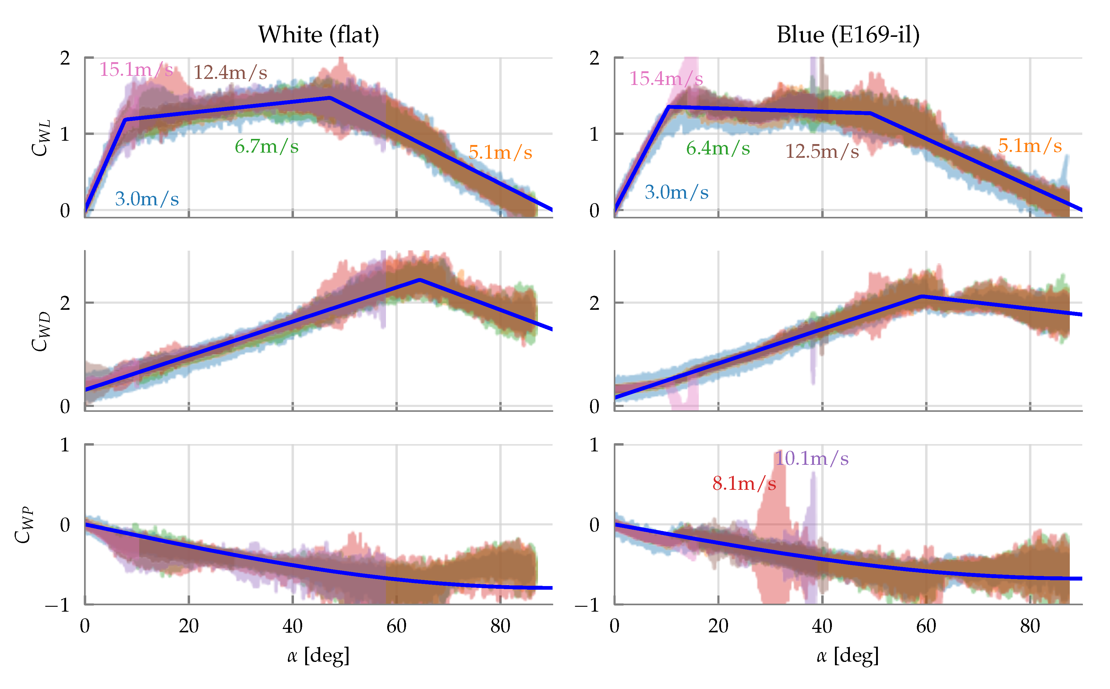
The measured aerodynamic coefficients are shown in Figure 5 as function of $\alpha$. From the figure, it can be seen that the stall behavior is less pronounced than for planar airfoils. This can partly be explained using the theoretical model in Appendix A. Also, the drag curves do not exhibit the usual curves of planar airfoils, which would have maximum drag at $\alpha =\pi /2$. In the case of the annular wing, the drag at $\alpha =\pi /2$ is small because of the curved surface that the incoming air can glide around, similar to a cylinder in cross-flow [64]. These behaviors were also observed in the early wind tunnel testing done in [53]. This could suggest that annular wing vehicles have better cross-wind resistance at hover than more traditional planar wing VTOLs [65]. The mean lift and drag curves are parametrized by a piece-wise linear fit, each assumed to be an odd and even function [66], respectively, where for positive angles of attack have the form:

$$\begin{array}{cc}\hfill {\overline{C}}_{WL}\left(\alpha \right)& =\left\{\begin{array}{cc}{c}_{l,\alpha ,0}\alpha \hfill & \alpha \in [0,{\alpha }_{l,0}]\hfill \\ c_{l,\alpha ,1}\alpha +c_{l,o,1}\hfill & \alpha \in [{\alpha }_{l,0},{\alpha }_{l,1}]\hfill \\ c_{l,\alpha ,2}\alpha +c_{l,o,2}\hfill & \alpha \in [{\alpha }_{l,1},\pi -{\alpha }_{l,1}]\hfill \\ -(c_{l,\alpha ,1}(\pi -\alpha )+c_{l,0,1})\hfill & \alpha \in [\pi -{\alpha }_{l,1},\pi -{\alpha }_{l,0}]\hfill \\ -c_{l,\alpha ,0}(\pi -\alpha )\hfill & \alpha \in [\pi -{\alpha }_{l,0},\pi ]\hfill \end{array}\right.\hfill \end{array}$$

(19)

$$\begin{array}{cc}\hfill {\overline{C}}_{WD}\left(\alpha \right)& =\left\{\begin{array}{cc}{c}_{d,\alpha ,0}\alpha +c_{d,0}\hfill & \alpha \in [0,{\alpha }_{d,0}]\hfill \\ c_{d,\alpha ,1}\alpha +c_{d,1}\hfill & \alpha \in [{\alpha }_{d,0},\pi /2]\hfill \\ c_{d,\alpha ,1}(\pi -\alpha )+c_{d,1}\hfill & \alpha \in [\pi /2,\pi -{\alpha }_{d,0}]\hfill \\ c_{d,\alpha ,0}(\pi -\alpha )+c_{d,0}\hfill & \alpha \in [\pi -{\alpha }_{d,0},\pi ]\hfill \end{array}\right.\hfill \end{array}$$

(20)

where the constants $c_{l,\alpha }$, $c_{l,0}$, ${\alpha }_l$, $c_{d,\alpha }$, $c_{d,0}$, and ${\alpha }_d$ are to be determined. For the lift coefficient, this is done by solving the following optimization

$$\begin{array}{c}\hfill \underset{{\alpha }_l}{minimize}\left(\underset{\begin{array}{c}{c}_{l,\alpha },c_{l,0}\\ \mathrm{s}.\mathrm{t}.c_{l,\alpha ,0}{\alpha }_{l,0}=c_{l,\alpha ,1}{\alpha }_{l,0}+c_{l,0,1}\\ c_{l,\alpha ,1}{\alpha }_{l,1}+c_{l,0,1}=c_{l,\alpha ,2}{\alpha }_{l,1}+c_{l,0,2}\end{array}}{minimize}S\left({[{\overline{C}}_{WL}\left({\alpha }^{\mathrm{meas}}\left[k\right]\right)-C_{WL}^{\mathrm{meas}}\left[k\right]]}_{k\in \mathcal{M}}\right)\right)\end{array}$$

(21)

where $S\left(·\right)$ is the Huber loss function for robustness against outliers [67] (alternatively, the sum of squares function or sum of absolute values can be used), $\mathcal{M}$ is the set of all measurements, and the superscript “$\mathrm{meas}$” is used to denote measured quantities. The constraints on the inner optimization are to ensure ${\overline{C}}_{WL}\left(·\right)$ is continuous in its argument $\alpha$. The inner optimization is convex and can be computed efficiently using CVXPY [68,69], while the outer optimization is not convex and is computed using the minimize routine in Scipy’s optimize package [70]. A similar procedure is performed for fitting the drag coefficient. For the pitching moment coefficient, a simple sinusoid term suffices:

$$\begin{array}{cc}\hfill {\overline{C}}_{WP}\left(\alpha \right)& =c_{p,\alpha }sin\left(\alpha \right)\hfill \end{array}$$

(22)

which can be determined easily from the measured data using a similar convex optimization routine.

The next step is to characterize the colored noise process (18). This is done by first discretizing (18) using an Euler approximation to yield

$$\begin{array}{c}\hfill {\eta }_{C_{WL}}[k+1]=a{\eta }_{C_{WL}}\left[k\right]+{\eta }_u\left[k\right]/T_s\end{array}$$

(23)

where $T_s=0.001\mathrm{s}$ is the sampling period and $a=1-T_s/\tau$. Then, the measured noise sequence is defined as

$$\begin{array}{c}\hfill {\eta }_{C_{WL}}^{\mathrm{meas}}\left[k\right]:=C_{WL}^{\mathrm{meas}}\left[k\right]-{\overline{C}}_{WL}\left({\alpha }^{\mathrm{meas}}\left[k\right]\right)\end{array}$$

(24)

Using this measured noise sequence, the parameter a and the variance of ${\eta }_u\left[k\right]$ can be computed using the autocorrelation (Yule-Walker) method as described in [71]. The distribution of ${\eta }_u\left[k\right]$ can be determined by plotting a histogram of

$$\begin{array}{c}\hfill {\eta }_u^{\mathrm{meas}}\left[k\right]:=({\eta }_{C_{WL}}^{\mathrm{meas}}\left[k\right]-a{\eta }_{C_{WL}}^{\mathrm{meas}}[k-1])Ts\end{array}$$

(25)

as shown in Figure 6, from which it can be observed that the distribution can be approximated by a Gaussian. With the distribution of ${\eta }_u\left[k\right]$ determined, and the parameter a determined earlier, the stochastic process (18) can be simulated and is shown in Figure 7. The simulated noisy sequence resembles the measured ${\eta }_{C_{WL}}^{\mathrm{meas}}\left[k\right]$, though a higher fidelity model can be realized by using a higher order autoregressive model. The fitted aerodynamic parameters can be found in

Table 2. Aerodynamic wing coefficients.

Parameter	Value
	White	Blue
$c_{l,\alpha ,0}$	8.78	7.45
$c_{l,\alpha ,1}$	0.42	−0.12
$c_{l,\alpha ,2}$	−1.97	−1.79
$c_{l,o,1}$	1.13	1.38
$c_{l,o,2}$	3.10	2.81
${\alpha }_{l,0}$	0.135	0.182
${\alpha }_{l,1}$	0.825	0.860
$c_{d,\alpha ,0}$	1.90	1.90
$c_{d,\alpha ,1}$	−2.16	−0.66
$c_{d,0}$	0.31	0.16
$c_{d,1}$	4.87	2.80
${\alpha }_{d,0}$	1.125	1.031
$\tau$	0.02
$\mathrm{Var}\left[{\eta }_u\left(t\right)\right]$	100

.

2.2.2. Propulsion

The rotor force and moment maps are modeled using the parametric models provided in [72]:

$$\begin{array}{cc}\hfill F_P^B(v_{A/B}^B,{\mathsf{\Omega }}_i)& :=R_R^B\left(v_{A/B}^B\right)\left[\begin{array}{c}{F}_{PH}(v_{A/B}^B,{\mathsf{\Omega }}_i)\\ F_{PS}(v_{A/B}^B,{\mathsf{\Omega }}_i)\\ F_{PT}(v_{A/B}^B,{\mathsf{\Omega }}_i)\end{array}\right]\hfill \end{array}$$

(26)

$$\begin{array}{cc}\hfill M_P^B(v_{A/B}^B,{\mathsf{\Omega }}_i)& :=R_R^B\left(v_{A/B}^B\right)\left[\begin{array}{c}{M}_{PR}(v_{A/B}^B,{\mathsf{\Omega }}_i)\\ M_{PP}(v_{A/B}^B,{\mathsf{\Omega }}_i)\\ M_{PQ}(v_{A/B}^B,{\mathsf{\Omega }}_i)\end{array}\right]\hfill \end{array}$$

(27)

where $F_{PH}\left(·\right)$ is the propeller H-force, $F_{PT}\left(·\right)$ is the propeller thrust, $F_{PS}\left(·\right)$ is the lateral/side force, and $M_{PR}\left(·\right)$, $M_{PP}\left(·\right)$, and $M_{PQ}\left(·\right)$ are the rolling, pitching and rotor torque, respectively. It is shown in (Section V, [72]), that these forces and moments can be written as

$$\begin{array}{cc}\hfill F_{PT}(v_{A/B}^B,{\mathsf{\Omega }}_i)& =\left(c_{PT,0}+c_{PT,{\lambda }_c}{\lambda }_c+c_{PT,{\lambda }_c^2}{\lambda }_c^2+c_{PT,{\mu }^2}{\mu }^2\right)(1/2)\rho {\left(\pi R\right)}^2{\left({\mathsf{\Omega }}_{i}R\right)}^2\hfill \end{array}$$

(28)

$$\begin{array}{cc}\hfill F_{PH}(v_{A/B}^B,{\mathsf{\Omega }}_i)& =\left(c_{PH,\mu }\mu \right)(1/2)\rho {\left(\pi R\right)}^2{\left({\mathsf{\Omega }}_{i}R\right)}^2\hfill \end{array}$$

(29)

$$\begin{array}{cc}\hfill F_{PS}(v_{A/B}^B,{\mathsf{\Omega }}_i)& \equiv 0\hfill \end{array}$$

(30)

$$\begin{array}{cc}\hfill M_{PR}(v_{A/B}^B,{\mathsf{\Omega }}_i)& =\left(c_{PR,\mu }\mu \right)(1/2)\rho {\left(\pi R\right)}^2{\left({\mathsf{\Omega }}_{i}R\right)}^{2}Rsign\left({\mathsf{\Omega }}_i\right)\hfill \end{array}$$

(31)

$$\begin{array}{cc}\hfill M_{PP}(v_{A/B}^B,{\mathsf{\Omega }}_i)& =\left(c_{PP,\mu }\mu +c_{PP,{\lambda }_c\mu }{\lambda }_c\mu \right)(1/2)\rho {\left(\pi R\right)}^2{\left({\mathsf{\Omega }}_{i}R\right)}^{2}R\hfill \end{array}$$

(32)

$$\begin{array}{cc}\hfill M_{PQ}(v_{A/B}^B,{\mathsf{\Omega }}_i)& =\left(c_{PQ,0}+c_{PQ,{\lambda }_c}{\lambda }_c+c_{PQ,{\lambda }_c^2}{\lambda }_c^2+c_{PQ,{\mu }^2}{\mu }^2\right)(1/2)\rho {\left(\pi R\right)}^2{\left({\mathsf{\Omega }}_{i}R\right)}^{2}Rsign(-{\mathsf{\Omega }}_i)\hfill \end{array}$$

(33)

where

$$\begin{array}{cc}\hfill {\lambda }_c& :=V_{\infty }cos\left(\alpha \right)/\left(\right|{\mathsf{\Omega }}_i\left|R\right)=-{v_{A/B}^B}_2/\left(\right|{\mathsf{\Omega }}_i\left|R\right)\hfill \end{array}$$

(34)

$$\begin{array}{cc}\hfill \mu & :=V_{\infty }sin\left(\alpha \right)/\left(\right|{\mathsf{\Omega }}_i\left|R\right)=\sqrt{{v_{A/B}^B}_0^2+{v_{A/B}^B}_1^2}/\left(\right|{\mathsf{\Omega }}_i\left|R\right)\hfill \end{array}$$

(35)

are the rotor climb and advance ratios for the ith rotor, respectively, R is the rotor radius, and the twelve $c_P$ constants are to be determined. Note, however, as mentioned in (Section V, [72]), the pitching moment model (32) may be inaccurate.

The constants are again determined by measuring the loads in a wind tunnel. The experimental set-up, shown in Figure 8, is the same as before with the same sweeping performed on $V_{\infty }$ and $\alpha$, but with two propellers mounted onto the vehicle. Two propellers were used because if all four were placed, and if all were sent the same rotation rate commands, the rotor torque $M_{PQ}$ and rolling moments $M_{PR}$ would cancel each other out. Furthermore, if only one was used, then this might cause a biased reading at that location. The propellers are commanded to sweep between 150 and 600 rad/s, sinusoidally with a period of $60\mathrm{s}$. The measured rotation rates ${\mathsf{\Omega }}_i$ are computed by the onboard STM32F4 microcontroller (see Section 3.1), which is then communicated to the host computer via the Laird RM024 radio.

The mean wing force and moment are subtracted from the measured loads using the identified model (19)–(22), to yield the measured rotor forces and moments from which the constants in the propeller model (28)–(33) are identified using a convex Huber regression [67]. The results are shown in Figure 9.

The thrust and rotor torque models fit very well, outperforming the standard hover model typically used in the drone literature [72], which is also shown for reference in Figure 9. The propeller H-force is very small for small angles of attack. The pitching moment model is inaccurate, however it can be shown that this is about an order of magnitude smaller than the pitching moment of the wing, and thus can be neglected. The slightly non-zero side force, and slightly inaccurate rolling and H-force models, may be the result of an asymmetrical induced flow observed by the rotor disk [73], resonance from the aeroelastic and vibration effects, or due to a slight misalignment of the load cell/vehicle. The numerical values of the aerodynamic coefficients can be found in

Table 3. Aerodynamic propeller coefficients.

Parameter	Value
$c_{PT,0}$	0.0368
$c_{PT,{\lambda }_c}$	−0.107
$c_{PT,{\mu }^2}$	0.060
$c_{PT,{\lambda }_c^2}$	−0.306
$c_{PH,\mu }$	0.0883
$c_{PQ,0}$	0.00483
$c_{PQ,{\lambda }_c}$	0.00202
$c_{PQ,{\mu }^2}$	−0.0299
$c_{PQ,{\lambda }_c^2}$	−0.111
$c_{PR,\mu }$	0.0594
$c_{PP,\mu }$	−0.00758
$c_{PP,{\lambda }_c\mu }$	0

.

3. Control System

3.1. Overview

The overall control architecture is based on a cascaded scheme as shown in Figure 10. A state estimator is used to fuse the sensor readings and is based on an extended Kalman filter (EKF) using an attitude reset scheme as described in [74], fusing the inertial measurement unit (IMU), magnetometer, pressure sensor and GPS. The state estimator provides an estimate of the body frame, denoted $\widehat{B}$, in the form of a position estimate $p_{\widehat{B}/I}^I$, velocity estimate $v_{\widehat{B}/I}^I$, and attitude estimate $R_{\widehat{B}}^I$. The estimate of the angular velocity, ${\omega }_{\widehat{B}/I}^{\widehat{B}}$, is read directly from the inertial measurement unit. The estimate of the propeller rotation rates, ${\widehat{\mathsf{\Omega }}}_i$, is measured using a timer on the STM32F4 and a pulse representing the zero-phase crossings that is provided by the SimonK firmware running on the ESCs [75,76]. GPS latency is also taken into account, by capturing the EKF estimate at the time of a measurement epoch to generate the innovation.

3.2. Position Controller

Consider the position trajectory of the reference frame, $p_{B^{\mathrm{ref}}/I}^I$, with corresponding time derivatives $v_{B^{\mathrm{ref}}/I}^I$ and $a_{B^{\mathrm{ref}}/I}^I$. A PID control loop is used to to generate the commanded acceleration $a_{B^{\mathrm{cmd}}/I}^I$ as follows:

$$\begin{array}{cc}\hfill a_{B^{\mathrm{cmd}}/I}^I& :=k_{p,p}(p_{B^{\mathrm{ref}}/I}^I-p_{\widehat{B}/I}^I)+k_{p,i}{\int }_0^t(p_{B^{\mathrm{ref}}/I}^I-p_{\widehat{B}/I}^I)\mathrm{d}t+k_{p,d}(v_{B^{\mathrm{ref}}/I}^I-v_{\widehat{B}/I}^I)+a_{B^{\mathrm{ref}}/I}^I\hfill \end{array}$$

(36)

where $k_{p,p}$, $k_{p,i}$, and $k_{p,d}$ are scalars representing the PID gains. This describes the acceleration of the frame $B^{\mathrm{cmd}}$. The orientation of $B^{\mathrm{cmd}}$ will be determined in the Outer Control Allocation block, described in the following section.

3.3. Outer Control Allocation

The commanded acceleration $a_{B^{\mathrm{cmd}}/I}^I$ is then fed to a control allocation scheme which determines the corresponding vehicle attitude, $R_{B^{\mathrm{cmd}}}^I$, and total collective vehicle thrust, $T^{\mathrm{cmd}}$, to achieve the commanded acceleration. To do so, the approximation $F_{PH}\approx 0$ is made, as the resulting tracking performance is adequate (see Section 5), although taking this into account may be subject for future work. Furthermore, as shown in Section 2.2.2, although the propeller H-force can become significant at high flight speeds at large angles of attack, this is not an operating condition in which the vehicle will spend much time.

Additionally, the approximation $v_{A/I}^{}\approx 0$ is made as no onboard wind speed estimator is available, and thus the feedback loop (36) will be used to compensate for this. Then, the control allocation problem can be formulated as follows:

$$\begin{array}{c}\hfill find{T}^{\mathrm{cmd}},R_{B^{\mathrm{cmd}}}^I\mathrm{s}.\mathrm{t}.R_{B^{\mathrm{cmd}}}^I{\overline{F}}_W^B(-R_I^{B^{\mathrm{cmd}}}{v}_{B^{\mathrm{ref}}/I}^I)+R_{B^{\mathrm{cmd}}}^I\left[\begin{array}{c}0\\ 0\\ T^{\mathrm{cmd}}\end{array}\right]=m\left(a_{B^{\mathrm{cmd}}/I}^I+g_{}^I\right)\end{array}$$

(37)

where ${\overline{F}}_W\left(·\right)=F_W\left(·\right)$ from (11), but with the aeroelastic noise component set to zero. This is done by first constructing an intermediate frame $A^{\mathrm{cmd}}$ (see Figure 11) as follows:

$$\begin{array}{cc}\hfill i_{A^{\mathrm{cmd}}}^I& :=\left\{\begin{array}{cc}n\left(v_{B^{\mathrm{ref}}/I}^I\right)\hfill & v_{B^{\mathrm{ref}}/I}^I\ne 0\hfill \\ \mathrm{arbitrary}\hfill & \mathrm{else}\hfill \end{array}\right.\hfill \end{array}$$

(38)

$$\begin{array}{cc}\hfill j_{A^{\mathrm{cmd}}}^I& :=\left\{\begin{array}{cc}n\left(i_{A^{\mathrm{cmd}}}^I\times \left(a_{B^{\mathrm{cmd}}/I}^I+g_{}^I\right)\right)\hfill & a_{B^{\mathrm{cmd}}/I}^I+g_{}^I\ne 0\hfill \\ \mathrm{arbitrary}(\mathrm{but}\mathrm{perpendicular}\mathrm{to}{i}_{A^{\mathrm{cmd}}}^I)\hfill & \mathrm{else}\hfill \end{array}\right.\hfill \end{array}$$

(39)

$$\begin{array}{cc}\hfill k_{A^{\mathrm{cmd}}}^I& :=i_A^I\times j_A^I\hfill \end{array}$$

(40)

Now the commanded force $m\left(a_{B^{\mathrm{cmd}}/I}^{}+g\right)$ must lie on the 2-dimension $i_{A^{\mathrm{cmd}}}^{},k_{A^{\mathrm{cmd}}}^{}$ plane. Let

$$\begin{array}{c}\hfill \left[\begin{array}{c}{f}_x(T^{\mathrm{cmd}},{\alpha }^{\mathrm{cmd}})\\ f_z(T^{\mathrm{cmd}},{\alpha }^{\mathrm{cmd}})\end{array}\right]:=\left[\begin{array}{c}-{\overline{C}}_{WD}\left({\alpha }^{\mathrm{cmd}}\right)\rho \Vert {v_{B^{\mathrm{ref}}/I}^I\Vert }^{2}S/2+T^{\mathrm{cmd}}cos\left({\alpha }^{\mathrm{cmd}}\right)\\ {\overline{C}}_{WL}\left({\alpha }^{\mathrm{cmd}}\right)\rho \Vert {v_{B^{\mathrm{ref}}/I}^I\Vert }^{2}S/2+T^{\mathrm{cmd}}sin\left({\alpha }^{\mathrm{cmd}}\right)\end{array}\right]\end{array}$$

(41)

The control allocation problem can thus be simplified to the following 2-dimensional problem:

$$\begin{array}{cc}\hfill find{T}^{\mathrm{cmd}},{\alpha }^{\mathrm{cmd}}\mathrm{s}.\mathrm{t}.\left[\begin{array}{c}{f}_x(T^{\mathrm{cmd}},{\alpha }^{\mathrm{cmd}})\\ f_z(T^{\mathrm{cmd}},{\alpha }^{\mathrm{cmd}})\end{array}\right]& =\left[\begin{array}{c}〈m\left(a_{B^{\mathrm{cmd}}/I}^I+g_{}^I\right),i_{A^{\mathrm{cmd}}}^I〉\\ 〈m\left(a_{B^{\mathrm{cmd}}/I}^I+g_{}^I\right),k_{A^{\mathrm{cmd}}}^I〉\end{array}\right]\hfill \end{array}$$

(42)

where $〈·,·〉$ is the inner product operator. A solution to the above always exists. This can be verified visually in Figure 12, where the range of (41) is plotted over all ${\alpha }^{\mathrm{cmd}}$ and $T^{\mathrm{cmd}}$. It can be observed that the range space of (41) is simply-connected (and also convex), and thus for sufficiently small commanded forces $f_x=〈m\left(a_{B^{\mathrm{cmd}}/I}^I+g_{}^I\right),i_{A^{\mathrm{cmd}}}^I〉,f_z=〈m\left(a_{B^{\mathrm{cmd}}/I}^I+g_{}^I\right),k_{A^{\mathrm{cmd}}}^I〉$, there will always be a solution $T^{\mathrm{cmd}},{\alpha }^{\mathrm{cmd}}$ that solves the allocation problem (42). Thus Newton’s method [67] is used to solve (42). Although ${\overline{C}}_{WL}\left(·\right)$ and ${\overline{C}}_{WD}\left(·\right)$ are continuous but not differentiable at the knot points, simple heuristics or the Secant method [4] can be used to circumvent this at the knots. Alternatively, the piece-wise linear curves can be made smooth by using a suitable sigmoid function at each knot.

With $T^{\mathrm{cmd}}$, ${\alpha }^{\mathrm{cmd}}$ determined, the rotation $R_{B^{\mathrm{cmd}}}^I$ in (37) can be constructed by

$$\begin{array}{cc}\hfill k_{B^{\mathrm{cmd}}}^I& :=cos\left({\alpha }^{\mathrm{cmd}}\right)i_{A^{\mathrm{cmd}}}^I+sin\left({\alpha }^{\mathrm{cmd}}\right)k_{A^{\mathrm{cmd}}}^I\hfill \end{array}$$

(43)

and the $i_{B^{\mathrm{cmd}}}^I$, $j_{B^{\mathrm{cmd}}}^I$ vectors can be suitably chosen to match the desired twist or yaw angle ${\psi }^{\mathrm{ref}}$. Note that this choice is arbitrary due to symmetry of the vehicle, and would not be possible for hybrid VTOL UAVs based on a planar airfoil, where coordinated turn maneuvers are required [47].

3.4. Feedforward Body Rates

For accurate tracking, the reference body rates need to be sent to the attitude controller, as shown in Figure 10. This is done by repeating the control allocation steps of Section 3.3 but using $a_{B^{\mathrm{ref}}/I}^I$ in place of $a_{B^{\mathrm{cmd}}/I}^I$ to generate the reference attitude $R_{B^{\mathrm{ref}}}^I$. The generated $R_{B^{\mathrm{ref}}}^I$ trajectory is then numerically differentiated using backwards differencing for rotations [77] to yield the reference body rates ${\omega }_{B^{\mathrm{ref}}/I}^{B^{\mathrm{ref}}}$. The feedforward angular accelerations may also be computed by numerically differentiating the feedforward body rates to yield ${\dot{\omega }}_{B^{\mathrm{ref}}/I}^{B^{\mathrm{ref}}}$.

3.5. Attitude Controller

The attitude error is the difference between the estimated body frame $\widehat{B}$ and the commanded body frame $B^{\mathrm{cmd}}$, represented as a rotation matrix as follows:

$$\begin{array}{cc}\hfill R_{\widehat{B}}^{B^{\mathrm{cmd}}}& :=R_I^{B^{\mathrm{cmd}}}{R}_{\widehat{B}}^I\hfill \end{array}$$

(44)

An intermediate error frame, called $\mathrm{tilt}$, is introduced, such that the attitude can be decomposed into a tilt and twist component:

$$\begin{array}{cc}\hfill R_{\widehat{B}}^{B^{\mathrm{cmd}}}& =R_{\mathrm{tilt}}^{B^{\mathrm{cmd}}}{R}_{\widehat{B}}^{\mathrm{tilt}}\hfill \end{array}$$

(45)

$$\begin{array}{cc}\hfill R_{\widehat{B}}^{\mathrm{tilt}}& =exp\left((*,*,0)\right)\hfill \end{array}$$

(46)

$$\begin{array}{cc}\hfill R_{\mathrm{tilt}}^{B^{\mathrm{cmd}}}& =exp\left((0,0,*)\right)\hfill \end{array}$$

(47)

where $exp\left(·\right)$ maps a rotation vector to the corresponding rotation matrix [60], $R_{\widehat{B}}^{\mathrm{tilt}}$ represents the tilt error, and $R_{\mathrm{tilt}}^{B^{\mathrm{cmd}}}$ represents a pure twist error. This decomposition can be done efficiently using unit-quaternions, see [78] or Appendix B. This is done because the twist error of the vehicle has no consequence on the tracking of the commanded acceleration, due to symmetry of the vehicle. Thus, the decomposition will be used to prioritize the tilt errors over twist errors, as follows: Let $q_{}^{}$ be the unit-quaternion representation of the rotation matrix $R_{}^{}$, and ${\overrightarrow{q}}_{}^{}$ its vector part. Then, the control law used for the attitude subsystem is given by

$$\begin{array}{cc}\hfill {\tau }^{\mathrm{cmd}}& =\underset{\mathrm{feedback}}{\underbrace{-k_{\mathrm{p},\mathrm{tilt}}{\overrightarrow{q}}_{\widehat{B}}^{\mathrm{tilt}}-k_{\mathrm{p},\psi }{\overrightarrow{q}}_{\widehat{B}}^{B^{\mathrm{cmd}}}-K_D{\omega }_{\widehat{B}/B^{\mathrm{ref}}}^{\widehat{B}}}}+\underset{\mathrm{feedforward}}{\underbrace{{\omega }_{B^{\mathrm{ref}}/I}^{\widehat{B}}\times J_B^B{\omega }_{B^{\mathrm{ref}}/I}^{\widehat{B}}+J_B^B{R}_{B^{\mathrm{ref}}}^{\widehat{B}}{\dot{\omega }}_{B^{\mathrm{ref}}/I}^{B^{\mathrm{ref}}}}}\hfill \end{array}$$

(48)

where $k_{\mathrm{p},\mathrm{tilt}},k_{\mathrm{p},\psi }$ are positive scalars representing the proportional gains for the tilt and twist errors, respectively, and $K_D$ is a positive definite matrix representing the derivative gains. The stability proof can be found in Appendix C. Another approach would be to replace the full attitude error term ${\overrightarrow{q}}_{\widehat{B}}^{B^{\mathrm{cmd}}}$ in (48) with the pure twist term ${\overrightarrow{q}}_{\mathrm{tilt}}^{B^{\mathrm{cmd}}}$, although the corresponding stability proof has not been found and is a suitable direction for future work. This approach differs from the tilt prioritization controller of [78,79], which includes (additional) feedback terms to linearize the angular dynamics.

3.6. Inner Control Allocation

The commanded body torques ${\tau }^{\mathrm{cmd}}$ and thrust $T^{\mathrm{cmd}}$ are then fed to a control allocation block which determines the corresponding propeller rates ${\mathsf{\Omega }}^{\mathrm{cmd}}$. Again, assuming that $v_{A/I}^{}=0$ as discussed in Section 3.3, this can be written formally as follows:

$$\begin{array}{c}\hfill find{\mathsf{\Omega }}^{\mathrm{cmd}}\mathrm{s}.\mathrm{t}.\left[\begin{array}{c}{\overline{M}}_W^B(-v_{B^{\mathrm{ref}}/I}^{B^{\mathrm{cmd}}})+\sum _{i=0}^3\left(M_P^B(-v_{B^{\mathrm{ref}}/I}^{B^{\mathrm{cmd}}},{\mathsf{\Omega }}_i^{\mathrm{cmd}})+p_{P_i/B}^B\times F_P^B(-v_{B^{\mathrm{ref}}/I}^{B^{\mathrm{cmd}}},{\mathsf{\Omega }}_i^{\mathrm{cmd}})\right)\\ \sum _{i=0}^3{F}_{PT}(-v_{B^{\mathrm{ref}}/I}^{B^{\mathrm{cmd}}},{\mathsf{\Omega }}_i^{\mathrm{cmd}})\end{array}\right]=\left[\begin{array}{c}{\tau }^{\mathrm{cmd}}\\ T^{\mathrm{cmd}}\end{array}\right]\end{array}$$

(49)

where the maps $F_{PT}\left(·\right),M_P^B\left(·\right),F_P^B\left(·\right)$ are given in (26)–(27), respectively, and ${\overline{M}}_W^B\left(·\right):=M_W^B\left(·\right)$ from (12), but with the aeroelastic noise component set to zero. To solve (49), the approximation of $F_{PH}\approx 0$ is made, as discussed in Section 3.3, and additionally

$$\begin{array}{cc}\hfill M_{PR}& \approx 0\hfill \end{array}$$

(50)

$$\begin{array}{cc}\hfill M_{PP}& \approx 0\hfill \end{array}$$

(51)

are made, although taking this into account is a suitable direction for future work. From a modeling perspective, the approximation $M_{PP}\approx 0$ is reasonable since as mentioned in Section 2.2, the pitching moment of the propeller is dominated by the wing. Next, the approximation $M_{PR}\approx 0$ is reasonable if the propeller rotation rate of a clockwise rotating propeller is roughly similar to that of a counter clockwise rotating propeller, such that the rolling moments approximately cancel each other out. From an experimental perspective, these approximations provide adequate tracking even at the high speed regime (see Section 5).

With these simplifications, (49) can be written equivalently as:

$$\begin{array}{c}\hfill find{\mathsf{\Omega }}^{\mathrm{cmd}}\mathrm{s}.\mathrm{t}.C{\left({\mathsf{\Omega }}^{\mathrm{cmd}}\right)}^2+D{\mathsf{\Omega }}^{\mathrm{cmd}}=C{\mathsf{\Omega }}_H^2-\left[\begin{array}{c}-{\overline{M}}_W^B\left(-v_{B^{\mathrm{ref}}/I}^{B^{\mathrm{cmd}}}\right)\\ -4\left(k_{T,{\lambda }_c^2}+k_{T,{\mu }^2}\right)\end{array}\right]\end{array}$$

(52)

where ${\left({\mathsf{\Omega }}^{\mathrm{cmd}}\right)}^2$ is performed element-wise,

$$\begin{array}{cc}\hfill C& =\left[\begin{array}{cccc}-l_{\mathrm{arm}}{k}_{T,0}/\sqrt{2}& -l_{\mathrm{arm}}{k}_{T,0}/\sqrt{2}& l_{\mathrm{arm}}{k}_{T,0}/\sqrt{2}& l_{\mathrm{arm}}{k}_{T,0}/\sqrt{2}\\ -l_{\mathrm{arm}}{k}_{T,0}/\sqrt{2}& l_{\mathrm{arm}}{k}_{T,0}/\sqrt{2}& l_{\mathrm{arm}}{k}_{T,0}/\sqrt{2}& -l_{\mathrm{arm}}{k}_{T,0}/\sqrt{2}\\ k_{\tau ,0}& -k_{\tau ,0}& k_{\tau ,0}& -k_{\tau ,0}\\ k_{T,0}& k_{T,0}& k_{T,0}& k_{T,0}\end{array}\right]\hfill \end{array}$$

(53)

$$\begin{array}{cc}\hfill D& =\left[\begin{array}{cccc}-l_{\mathrm{arm}}{k}_{T,{\lambda }_c}/\sqrt{2}& -l_{\mathrm{arm}}{k}_{T,{\lambda }_c}/\sqrt{2}& l_{\mathrm{arm}}{k}_{T,{\lambda }_c}/\sqrt{2}& l_{\mathrm{arm}}{k}_{T,{\lambda }_c}/\sqrt{2}\\ -l_{\mathrm{arm}}{k}_{T,{\lambda }_c}/\sqrt{2}& l_{\mathrm{arm}}{k}_{T,{\lambda }_c}/\sqrt{2}& l_{\mathrm{arm}}{k}_{T,{\lambda }_c}/\sqrt{2}& -l_{\mathrm{arm}}{k}_{T,{\lambda }_c}/\sqrt{2}\\ k_{\tau ,{\lambda }_c}& -k_{\tau ,{\lambda }_c}& k_{\tau ,{\lambda }_c}& -k_{\tau ,{\lambda }_c}\\ k_{T,{\lambda }_c}& k_{T,{\lambda }_c}& k_{T,{\lambda }_c}& k_{T,{\lambda }_c}\end{array}\right]\hfill \end{array}$$

(54)

where $l_{\mathrm{arm}}$ is the distance between the vehicle center and a propeller’s center,

$$\begin{array}{cc}\hfill k_{T,0}& :=c_{PT,0}(1/2)\rho {\left(\pi R\right)}^2{R}^2\hfill \end{array}$$

(55)

$$\begin{array}{cc}\hfill k_{T,{\lambda }_c}& :=c_{PT,{\lambda }_c}(1/2)\rho {\left(\pi R\right)}^{2}R\Vert v_{B^{\mathrm{ref}}/I}^I\Vert cos\left({\alpha }^{\mathrm{cmd}}\right)\hfill \end{array}$$

(56)

$$\begin{array}{cc}\hfill k_{T,{\mu }^2}& :=c_{PT,{\mu }^2}(1/2)\rho {\left(\pi R\right)}^2{\left(\Vert v_{B^{\mathrm{ref}}/I}^I\Vert sin\left({\alpha }^{\mathrm{cmd}}\right)\right)}^2\hfill \end{array}$$

(57)

$$\begin{array}{cc}\hfill k_{T,{\lambda }_c^2}& :=c_{PT,{\lambda }_c^2}(1/2)\rho {\left(\pi R\right)}^2{\left(\Vert v_{B^{\mathrm{ref}}/I}^I\Vert cos\left({\alpha }^{\mathrm{cmd}}\right)\right)}^2\hfill \end{array}$$

(58)

$$\begin{array}{cc}\hfill k_{\tau ,0}& :=c_{PQ,0}(1/2)\rho {\left(\pi R\right)}^2{R}^3\hfill \end{array}$$

(59)

$$\begin{array}{cc}\hfill k_{\tau ,{\lambda }_c}& :=c_{PQ,{\lambda }_c}(1/2)\rho {\left(\pi R\right)}^2{R}^2\Vert v_{B^{\mathrm{ref}}/I}^I\Vert cos\left({\alpha }^{\mathrm{cmd}}\right)\hfill \end{array}$$

(60)

are defined for brevity, and where ${\mathsf{\Omega }}_H$ is the standard quadrotor hover solution:

$$\begin{array}{c}\hfill {\mathsf{\Omega }}_H^2:=C^{-1}\left[\begin{array}{c}{\tau }^{\mathrm{cmd}}\\ T^{\mathrm{cmd}}\end{array}\right]\end{array}$$

(61)

Note that the C and D matrices are defined if the body frame B is as shown in Figure 3, modulo the ordering of the rotors. If they are instead aligned with the rotor arms, as is typically done in the quadrotor literature, then:

$$\begin{array}{c}\hfill C=\left[\begin{array}{cccc}0& -l_{\mathrm{arm}}{k}_{T,0}& 0& l_{\mathrm{arm}}{k}_{T,0}\\ -l_{\mathrm{arm}}{k}_{T,0}& 0& l_{\mathrm{arm}}{k}_{T,0}& 0\\ k_{\tau ,0}& -k_{\tau ,0}& k_{\tau ,0}& -k_{\tau ,0}\\ k_{T,0}& k_{T,0}& k_{T,0}& k_{T,0}\end{array}\right],D=\left[\begin{array}{cccc}0& -l_{\mathrm{arm}}{k}_{T,{\lambda }_c}& 0& l_{\mathrm{arm}}{k}_{T,{\lambda }_c}\\ -l_{\mathrm{arm}}{k}_{T,{\lambda }_c}& 0& l_{\mathrm{arm}}{k}_{T,{\lambda }_c}& 0\\ k_{\tau ,{\lambda }_c}& -k_{\tau ,{\lambda }_c}& k_{\tau ,{\lambda }_c}& -k_{\tau ,{\lambda }_c}\\ k_{T,{\lambda }_c}& k_{T,{\lambda }_c}& k_{T,{\lambda }_c}& k_{T,{\lambda }_c}\end{array}\right]\end{array}$$

(62)

One way to solve (52) is to use Newton’s method, as done in the outer loop control allocation block. However, this results in excessive computation, requiring the inverse of a 4 × 4 Hessian matrix. As an alternative, let

$$\begin{array}{c}\hfill f\left(\mathsf{\Omega }\right):=\sqrt{{\mathsf{\Omega }}_H^2-C^{-1}D\mathsf{\Omega }-C^{-1}\left[\begin{array}{c}-{\overline{M}}_W^B\left(-v_{B^{\mathrm{ref}}/I}^{B^{\mathrm{cmd}}}\right)\\ -4\left(k_{T,{\lambda }_c^2}+k_{T,{\mu }^2}\right)\end{array}\right]}\end{array}$$

(63)

where the square-root is applied element-wise. The goal is to find the fixed point ${\mathsf{\Omega }}^{\mathrm{cmd}}:={\mathsf{\Omega }}^{*}$ such that ${\mathsf{\Omega }}^{*}=f\left({\mathsf{\Omega }}^{*}\right)$. Note that

$$\begin{array}{cc}\hfill ∥{\left.\frac{\partial f\left(\mathsf{\Omega }\right)}{\partial \mathsf{\Omega }}\right|}_{{\mathsf{\Omega }}^{*}}∥& =(1/2)∥diag\left(1/f{\left({\mathsf{\Omega }}^{*}\right)}_0,1/f{\left({\mathsf{\Omega }}^{*}\right)}_1,1/f{\left({\mathsf{\Omega }}^{*}\right)}_2,1/f{\left({\mathsf{\Omega }}^{*}\right)}_3\right)(-C^{-1}D)∥\hfill \end{array}$$

(64)

$$\begin{array}{cc}\hfill & =(1/2)∥diag\left(1/{\mathsf{\Omega }}_0^{*},1/{\mathsf{\Omega }}_1^{*},1/{\mathsf{\Omega }}_2^{*},1/{\mathsf{\Omega }}_3^{*}\right)(-C^{-1}D)∥\hfill \end{array}$$

(65)

$$\begin{array}{cc}\hfill & \le ∥C^{-1}D∥/\left(2\underset{i}{min}{\mathsf{\Omega }}_i^{*}\right)\hfill \end{array}$$

(66)

$$\begin{array}{cc}\hfill & =max\left\{|k_{T,{\lambda }_c}/k_{T,0}|,|k_{\tau ,{\lambda }_c}/k_{\tau ,0}|\right\}/\left(2\underset{i}{min}{\mathsf{\Omega }}_i^{*}\right)\hfill \end{array}$$

(67)

$$\begin{array}{cc}\hfill & =(1/2)max\left\{|c_{PT,{\lambda }_c}/c_{PT,0}|,|c_{PQ,{\lambda }_c}/c_{PQ,0}|\right\}\underset{i}{max}\left|{{\lambda }_c^{*}}_i\right|\hfill \end{array}$$

(68)

where the norm applied to the Jacobian is the induced matrix 2-norm, and ${{\lambda }_c^{*}}_i:=\Vert v_{B^{\mathrm{ref}}/I}^I\Vert cos\left({\alpha }^{\mathrm{cmd}}\right)/\left({\mathsf{\Omega }}_i^{*}R\right)$. $f\left(·\right)$ will be a local contraction mapping if (68) is strictly less than 1 [80]. This will always be the case for a sufficiently small operating region in the climb ratio ${\lambda }_c$. For example, using the parameter values from Table 3, this means that for the annular wing vehicle, the operating ${\lambda }_c$ ratio must be less than 0.68. This is a very extreme operating condition and will not be encountered in practice, as a climb ratio of 0.2 corresponds roughly to when UAV propellers produce zero thrust [72]. Since $f\left(·\right)$ is a local contraction about the solution, then by Banach’s Fixed Point Theorem [80], Algorithm 1 can be used to find the fixed point ${\mathsf{\Omega }}^{*}$.

Algorithm 1: Iterative algorithm to solve the inner control allocation problem (52)

In practice, Algorithm 1 works for ${\lambda }_c$ larger than 0.68, as Banach’s Fixed Point Theorem is only a sufficiency condition, although such a scenario is not so interesting as this would not be encountered in practice. In practice, Algorithm 1 is initialized with the previous time-step’s solution.

See Figure 13 for a simulation of Algorithm 1, where the commanded operating condition is the target operating speed of $\Vert v_{B^{\mathrm{ref}}/I}^I\Vert =10\mathrm{m}/\mathrm{s}$. The hover solution ${\mathsf{\Omega }}_H$ is used to initialize Algorithm 1 in this case. This figure demonstrates two things: at this high speed, the hover solution is off by a large amount, as the propellers need to rotate faster to produce the same thrust (under predominantly axial flow), as evident during the modeling done in Section 2.2. The second is that Algorithm 1 converges very quickly, often only requiring a couple of iterations in practice. Figure 14 shows the closed loop tracking results when using the proposed scheme presented herein, and if the hover solution ${\mathsf{\Omega }}_H$ were applied instead (both schema use the same feedback control gains as used in the experiments in Section 5). Here it can be seen that the proposed scheme tracks the desired high-speed maneuver accurately, whereas the hover solution fails to even hit the target reference speed of $10\mathrm{m}/\mathrm{s}$. Of course, the standard hover approach can be improved with further tuning (i.e., increasing) the feedback gains, however doing so will have undesirable consequences, such as causing the system to be more sensitive to disturbances and noise.

3.7. Motor Controller

The commanded propeller rates ${\mathsf{\Omega }}^{\mathrm{cmd}}$ are then fed to the motor controller, which uses a combination of a PI controller for feedback compensation and a feedforward term as follows:

$$\begin{array}{c}\hfill u_i^{\mathrm{cmd}}:=\underset{\mathrm{feedback}}{\underbrace{k_{p,\mathsf{\Omega }}({\widehat{\mathsf{\Omega }}}_i-{\mathsf{\Omega }}_i^{\mathrm{cmd}})+k_{i,\mathsf{\Omega }}{\int }_0^t({\widehat{\mathsf{\Omega }}}_i-{\mathsf{\Omega }}_i^{\mathrm{cmd}})\mathrm{d}t}}+\underset{\mathrm{feedforward}}{\underbrace{(R_m/K_m)M_{PQ}(-v_{B^{\mathrm{ref}}/I}^{B^{\mathrm{cmd}}},{\mathsf{\Omega }}_i^{\mathrm{cmd}})}}\end{array}$$

(69)

where $k_{p,\mathsf{\Omega }},k_{i,\mathsf{\Omega }}$ are the PI gains. The feedforward term is again necessary for accurate tracking and compensation of the propeller torque that is encountered in both hover and forward flight.

3.8. Trajectories

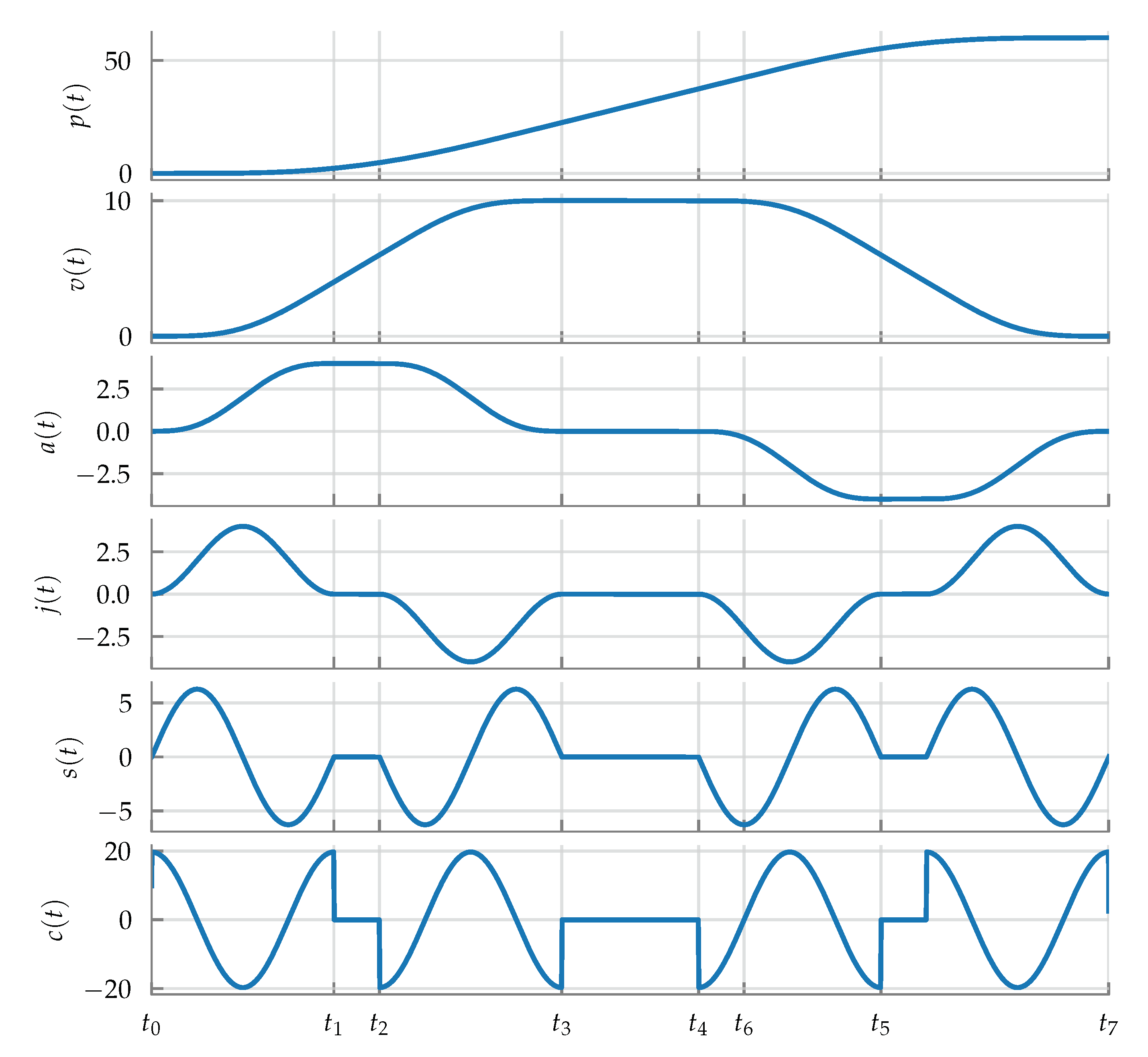
It can be shown that the current draw of the motors is a function of the crackle (5th derivative) of the vehicle’s position trajectory. Thus, to minimize current spikes, trajectories that have bounded crackle (see Figure 15) are used to generate the reference position trajectory and its derivatives. This is done by using the harmonic jerk model of [81]:

$$\begin{array}{c}\hfill j^{\mathrm{ref}}\left(t\right):=\left\{\begin{array}{cc}{j}_{\max }\left(1-cos\left(2\pi (t-t_i)/T_j\right)\right)/2\hfill & t\in [t_0,t_1],t\in [t_6,t_7]\hfill \\ 0\hfill & t\in [t_1,t_2],t\in [t_3,t_4],t\in [t_5,t_6]\hfill \\ -j_{\max }\left(1-cos\left(2\pi (t-t_i)/T_j\right)\right)/2\hfill & t\in [t_2,t_3],t\in [t_4,t_5]\hfill \end{array}\right.\end{array}$$

(70)

where $j_{\max }$, $T_J$ are design parameters, and $t_i$ is the initial time instant of the corresponding segment. These parameters are selected so that a desired position set-point is achieved in each axis.

4. Software Implementation

An important aspect of the control system is the software architecture used to implement it. The approach here uses the NuttX real-time operating system (RTOS), which is a light-weight, POSIX compliant RTOS [82]. The POSIX compliance is the critical ingredient used to achieve high fidelity software-in-the-loop simulations, as the application software written for the embedded platform can also be compiled to run on a host’s POSIX compliant personal computer (PC) (such as a distribution based on GNU/Linux). This allows for certain bugs such as stack overflows, race-conditions arising from context switches and interprocess communication (IPC) to be simulated [83], and thus can be caught in advance instead of having to debug software directly on the embedded platform. This is unlike the approach of [22,84], where only the control algorithms are simulated as common library routines, or a Simulink (or equivalent) approach [7,20,37,85,86,87,88,89,90], where there is a clear separation or distinction between simulated code and code implemented on the embedded platform.

The software architecture employed is shown in Figure 16. The onboard task can run either on the embedded platform, or on the host PC for simulation. The onboard task is oblivious to whether it is being run as a simulation or not. It reads in sensor values using dedicated polling threads through the virtual file interface via the device drivers [83], and then sends the motor voltages $u^{\mathrm{cmd}}$ via the same interface. The device drivers provide the needed abstraction, where they are implemented to communicate with the real sensors and actuators on NuttX. For simulation, they are implemented on a GNU/Linux machine via kernel modules [91], which relay information to and from the simulator process.

All of the control laws discussed in Section 3 are implemented in the fast thread running within the onboard main task. It runs at a fixed frequency of $500\mathrm{Hz}$ that is controlled by a dedicated timer driver /dev/timer0 via signalling [83]. The slow thread communicates with the radio device for sending telemetry and receiving high level commands from the user (such as takeoff, land, or fly a certain trajectory). It is also responsible for monitoring for any sensor faults and bringing the vehicle to an emergency land state. The offboard task runs only on the host PC and runs regardless of whether a simulation or real experiment is being run. The offboard task communicates with the host radio device for sending high level commands to the vehicle and receiving telemetry. It also provides the user with a real time visualization of the received telemetry data. The simulator task runs on the host PC, using the system model described in Section 2 to drive the ordinary differential equation (ODE) solver [92].

5. Experimental Results

The experiments were performed outdoors; a video can be found at https://youtu.be/ULc63HrgPro. The experiments were performed in conditions with wind speeds of $2\mathrm{m}/\mathrm{s}$ and occasional wind gusts of up to $5\mathrm{m}/\mathrm{s}$, according to local weather forecasts provided by [93].

Two experiments are performed. The first is a straight line trajectory, shown in Figure 17 and Figure 18, where the vehicle is commanded to traverse $60\mathrm{m}$ reaching a top speed of $10\mathrm{m}/\mathrm{s}$. The results show good tracking of the position reference, even at the high-speed part of the trajectory. No significant altitude fluctuations were encountered, even during the transition. The vehicle’s tilt angle computed by

$$\begin{array}{cc}\hfill \mathrm{tilt}\mathrm{angle}& =arccos\left({R_{\widehat{B}}^I}_{2,2}\right)\hfill \end{array}$$

(71)

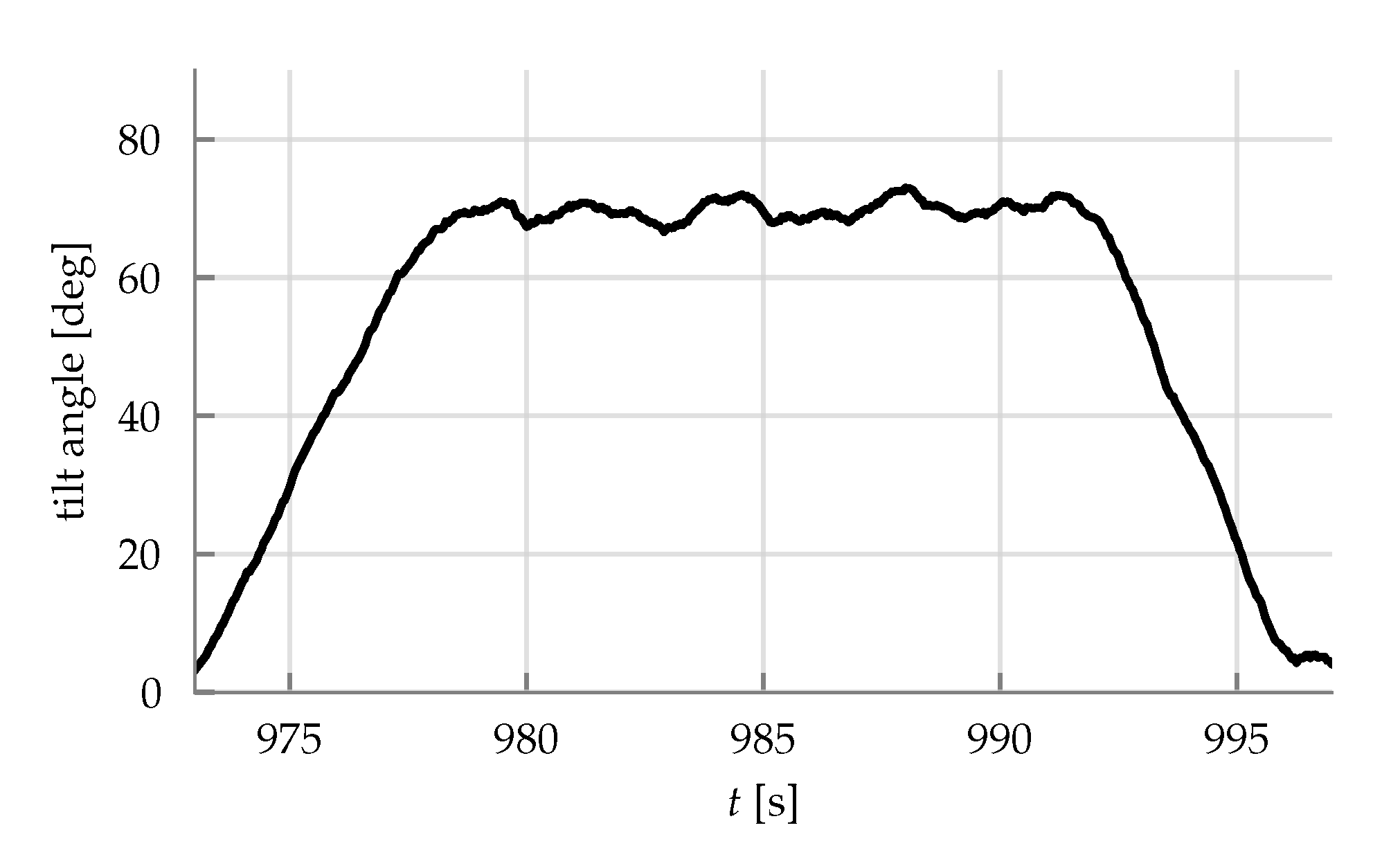
i.e., the arccos of the last entry of the rotation matrix, is shown in Figure 19. The tilt angle varies between 0 and 80 degrees during the straight line maneuver. The forward and reverse pass differ due to external wind disturbances and possibly by asymmetries due to manufacturing imperfections.

The second trajectory is shown in Figure 20, Figure 21 and Figure 22, where the vehicle is commanded to travel in a circle of radius $10\mathrm{m}$ at a speed of $10\mathrm{m}/\mathrm{s}$. The results again show good tracking of the reference trajectory throughout the high-speed maneuver. Figure 22 shows that the vehicle’s k-axis is not tangent with the circle, as the annular wing is not only providing lift to counteract gravity, but also generating lift in the plane of the circle to provide the required centripetal acceleration, mixed of course with the rotor thrust. This mixing is done automatically by the outer control allocation block as discussed in Section 3.

6. Conclusions

A quadrotor with an annular wing has been presented that enhances human safety and can provide efficient forward flight. The annular wing and propellers have been characterized through wind tunnel experiments. The designed model-based control system accounts for the dominant aerodynamics of the propellers under general oblique flow conditions using an iterative algorithm, and utilizes a tilt-prioritized attitude controller that takes advantage of the symmetry of the vehicle. The control system has been demonstrated through outdoor experiments and shown to provide accurate transition maneuvers and high-speed trajectory tracking.

The iterative control allocation algorithm presented in Section 3.6 can be applied to any quadrotor vehicle, and is a suitable direction for future work for improving tracking performance at high speeds. A more optimized vehicle design, using lighter and more rigid materials, is a suitable direction for future work. Other directions include taking into account the propeller H-force and incorporating an onboard wind speed estimate in the control allocation blocks, and seeking the attitude control stability proof when a pure twist term is used in the control law (48). Other directions include performing a rigorous comparison on cross-wind resistance and noise emission of the proposed annular wing vehicle with conventional planar wing tail-sitters.

References

- Campbell, J.P. Research on VTOL and STOL aircraft in the United States. In Advances in Aeronautical Sciences: Proceedings of the First International Congress in the Aeronautical Sciences, Madrid, Spain, 8–13 September 1958; Elsevier: Amsterdam, The Netherlands, 2014; p. 845. [Google Scholar]
- Anderson, S.B. Historical Overview of V/STOL Aircraft Technology; NASA-TM-81280, A-8511; NASA Ames Research Center: Moffett Field, CA, USA, 1981. [Google Scholar]
- Sigala, A.; Langhals, B. Applications of Unmanned Aerial Systems (UAS): A Delphi Study Projecting Future UAS Missions and Relevant Challenges. Drones 2020, 4, 8. [Google Scholar] [CrossRef] [Green Version]
- Saeed, A.S.; Younes, A.B.; Islam, S.; Dias, J.; Seneviratne, L.; Cai, G. A review on the platform design, dynamic modeling and control of hybrid UAVs. In Proceedings of the International Conference on Unmanned Aircraft Systems, Denver, CO, USA, 9–12 June 2015; pp. 806–815. [Google Scholar] [CrossRef]
- Xu, J. Design Perspectives on Delivery Drones; RAND: Santa Monica, CA, USA, 2017. [Google Scholar]
- Woods, R.J. Convertiplanes and Other VTOL Aircraft; Technical Report, SAE Technical Paper; SAE International: Warrendale, MI, USA, 1957. [Google Scholar] [CrossRef]
- Stone, R.; Clarke, G. The T-Wing: A VTOL UAV for Defense and Civilian Applications; University of Sydney: Sydney, Australia, 2001. [Google Scholar]
- Hochstenbach, M.; Notteboom, C.; Theys, B.; Schutter, J.D. Design and Control of an Unmanned Aerial Vehicle for Autonomous Parcel Delivery with Transition from Vertical Take-off to Forward Flight— VertiKUL, a Quadcopter Tailsitter. Int. J. Micro Air Veh. 2015, 7, 395–405. [Google Scholar] [CrossRef] [Green Version]
- Saeed, A.S.; Younes, A.B.; Cai, C.; Cai, G. A survey of hybrid Unmanned Aerial Vehicles. Prog. Aerospace Sci. 2018, 98, 91–105. [Google Scholar] [CrossRef]
- De Wagter, C.; Ruijsink, R.; Smeur, E.J.J.; van Hecke, K.G.; van Tienen, F.; van der Horst, E.; Remes, B.D.W. Design, control, and visual navigation of the DelftaCopter VTOL tail-sitter UAV. J. Field Robot. 2018, 35, 937–960. [Google Scholar] [CrossRef] [Green Version]
- Swarnkar, S.; Parwana, H.; Kothari, M.; Abhishek, A. Biplane-Quadrotor Tail-Sitter UAV: Flight Dynamics and Control. J. Guid. Control Dyn. 2018, 41, 1049–1067. [Google Scholar] [CrossRef]
- News, B. Toddler’s Eyeball Sliced in Half by Drone Propeller. Available online: http://www.bbc.com/news/uk-england-hereford-worcester-34936739 (accessed on 1 January 2020).
- Alphonse, V.D.; Kemper, A.R.; Rowson, S.; Duma, S.M. Eye injury risk associated with remote control toy helicopter blades. Biomed. Sci. Instrum. 2012, 48, 20–26. [Google Scholar]
- DroneImpact-T0005—3200 fps to 25 fps (Pork, Carbon Propeller, 9 m/s). Available online: https://youtu.be/QQoTQZcwZWE (accessed on 13 April 2020).
- MythBusters: Flights of Fantasy. Episode 230, Discovery Channel. 2015. Available online: https://go.discovery.com/tv-shows/mythbusters (accessed on 1 January 2020).
- Arterburn, D.R.; Duling, C.T.; Goli, N.R. Ground Collision Severity Standards for UAS Operating in the National Airspace System (NAS). In Proceedings of the 17th AIAA Aviation Technology, Integration, and Operations Conference, Denver, CO, USA, 5–9 June 2017. [Google Scholar] [CrossRef]
- Johnson, J.A.; Svach, M.R.; Brown, L.H. Drone and Other Hobbyist Aircraft Injuries Seen in U.S. Emergency Departments, 2010–2017. Am. J. Prev. Med. 2019, 57, 826–829. [Google Scholar] [CrossRef]
- Young, L.; Aiken, E.; Johnson, J.; Demblewski, R.; Andrews, J.; Klem, J. New Concepts and Perspectives on Micro-Rotorcraft and Small Autonomous Rotary-Wing Vehicles. In Proceedings of the AIAA Applied Aerodynamics Conference, Chicago, IL, USA, 28 June–1 July 2010. [Google Scholar] [CrossRef] [Green Version]
- Waibel, M.; Keays, B.; Augugliaro, F. Drone Shows: Creative Potential and Best Practices; Technical Report; ETH Zurich: Zurich, Switzerland, 2017. [Google Scholar] [CrossRef]
- Theys, B.; De Vos, G.; De Schutter, J. A control approach for transitioning VTOL UAVs with continuously varying transition angle and controlled by differential thrust. In Proceedings of the International Conference on Unmanned Aircraft Systems, Arlington, VA, USA, 7–10 June 2016; pp. 118–125. [Google Scholar] [CrossRef]
- Gill, R. Flying Ring Robot Can Fly on Its Side. Available online: https://robohub.org/flying-ring-robot-can-fly-on-its-side/ (accessed on 1 January 2016).
- Lupashin, S.; Hehn, M.; Mueller, M.W.; Schoellig, A.P.; Sherback, M.; D’Andrea, R. A platform for aerial robotics research and demonstration: The Flying Machine Arena. Mechatronics 2014, 24, 41–54. [Google Scholar] [CrossRef]
- Wilke, J. A Drone Program Taking Off. Available online: https://blog.aboutamazon.com/transportation/a-drone-program-taking-flight (accessed on 1 January 2020).
- Johnson, E.; Turbe, M.; Wu, A.; Kannan, S.; Neidhoefer, J. Flight Results of Autonomous Fixed-Wing UAV Transitions to and from Stationary Hover. In Proceedings of the AIAA Guidance, Navigation, and Control Conference and Exhibit, Keystone, CO, USA, 21–24 August 2006. [Google Scholar] [CrossRef] [Green Version]
- Kita, K.; Konno, A.; Uchiyama, M. Transition between Level Flight and Hovering of a Tail-Sitter Vertical Takeoff and Landing Aerial Robot. Adv. Robot. 2010, 24, 763–781. [Google Scholar] [CrossRef]
- Stone, R.H. Control architecture for a tail-sitter unmanned air vehicle. In Proceedings of the Asian Control Conference, Melbourne, Australia, 20–23 July 2004; Volume 2, pp. 736–744. [Google Scholar]
- Stone, R.H.; Anderson, P.; Hutchison, C.; Tsai, A.; Gibbens, P.; Wong, K.C. Flight Testing of the T-Wing Tail-Sitter Unmanned Air Vehicle. J. Aircraft 2008, 45, 673–685. [Google Scholar] [CrossRef]
- Argyle, M.E.; Beard, R.W.; Morris, S. The Vertical Bat tail-sitter: Dynamic model and control architecture. In Proceedings of the American Control Conference, Washington, DC, USA, 17–19 June 2013; pp. 806–811. [Google Scholar] [CrossRef]
- Verling, S.; Weibel, B.; Boosfeld, M.; Alexis, K.; Burri, M.; Siegwart, R. Full Attitude Control of a VTOL tailsitter UAV. In Proceedings of the IEEE International Conference on Robotics and Automation, Stockholm, Sweden, 16–21 May 2016; pp. 3006–3012. [Google Scholar] [CrossRef] [Green Version]
- Udagawa, T.; Chisaka, T.; Ishii, R. Tail-sitter VTOL-UAV—Research project overview. In Proceedings of the 24th Congress of International Council of the Aeronautical Sciences, Yokohama, Japan, 29 August–3 September 2004. [Google Scholar]
- Sinha, P.; Esden-Tempski, P.; Forrette, C.A.; Gibboney, J.K.; Horn, G.M. Versatile, modular, extensible vtol aerial platform with autonomous flight mode transitions. In Proceedings of the IEEE Aerospace Conference, Big Sky, MT, USA, 3–10 March 2012; pp. 1–17. [Google Scholar] [CrossRef]
- Oosedo, A.; Abiko, S.; Konno, A.; Koizumi, T.; Furui, T.; Uchiyama, M. Development of a quad rotor tail-sitter VTOL UAV without control surfaces and experimental verification. In Proceedings of the IEEE International Conference on Robotics and Automation, Karlsruhe, Germany, 6–10 May 2013; pp. 317–322. [Google Scholar] [CrossRef]
- Oosedo, A.; Abiko, S.; Konno, A.; Uchiyama, M. Optimal transition from hovering to level-flight of a quadrotor tail-sitter UAV. Auton. Robots 2017, 41, 1143–1159. [Google Scholar] [CrossRef]
- Wang, Y.; Lyu, X.; Gu, H.; Shen, S.; Li, Z.; Zhang, F. Design, implementation and verification of a quadrotor tail-sitter VTOL UAV. In Proceedings of the International Conference on Unmanned Aircraft Systems, Miami, FL, USA, 13–16 June 2017; pp. 462–471. [Google Scholar] [CrossRef]
- Lyu, X.; Gu, H.; Wang, Y.; Li, Z.; Shen, S.; Zhang, F. Design and implementation of a quadrotor tail-sitter VTOL UAV. In Proceedings of the IEEE International Conference on Robotics and Automation, Singapore, 29 May–3 June 2017; pp. 3924–3930. [Google Scholar] [CrossRef]
- Forshaw, J.L.; Lappas, V.J.; Briggs, P. Transitional Control Architecture and Methodology for a Twin Rotor Tailsitter. J. Guid. Control Dyn. 2014, 37, 1289–1298. [Google Scholar] [CrossRef]
- Wang, X.; Chen, Z.; Yuan, Z. Modeling and control of an agile tail-sitter aircraft. J. Frankl. Inst. 2015, 352, 5437–5472. [Google Scholar] [CrossRef] [Green Version]
- Jung, Y.; Cho, S.; Shim, D.H. A Comprehensive Flight Control Design and Experiment of a Tail-Sitter UAV. In Proceedings of the AIAA Guidance, Navigation, and Control Conference, Boston, MA, USA, 19–22 August 2013. [Google Scholar] [CrossRef]
- Bapst, R.; Ritz, R.; Meier, L.; Pollefeys, M. Design and implementation of an unmanned tail-sitter. In Proceedings of the IEEE/RSJ International Conference on Intelligent Robots and Systems, Hamburg, Germany, 28 September–2 October 2015; pp. 1885–1890. [Google Scholar] [CrossRef]
- Hogge, J.V. Development of a Miniature VTOL Tail-Sitter Unmanned Aerial Vehicle; Brigham Young University: Provo, UT, USA, 2008. [Google Scholar]
- Kubo, D.; Suzuki, S. Tail-Sitter Vertical Takeoff and Landing Unmanned Aerial Vehicle: Transitional Flight Analysis. J. Aircraft 2008, 45, 292–297. [Google Scholar] [CrossRef]
- Moore, M. NASA Puffin Electric Tailsitter VTOL Concept. In Proceedings of the AIAA Aviation Technology, Integration, and Operations Conference, Fort Worth, TX, USA, 13–15 September 2010. [Google Scholar] [CrossRef] [Green Version]
- Matsumoto, T.; Kita, K.; Suzuki, R.; Oosedo, A.; Go, K.; Hoshino, Y.; Konno, A.; Uchiyama, M. A hovering control strategy for a tail-sitter VTOL UAV that increases stability against large disturbance. In Proceedings of the IEEE International Conference on Robotics and Automation, Anchorage, AK, USA, 3–7 May 2010; pp. 54–59. [Google Scholar] [CrossRef]
- Suzuki, R.; Matsumoto, T.; Konno, A.; Hoshino, Y.; Go, K.; Oosedo, A.; Uchiyama, M. Teleoperation of a tail-sitter VTOL UAV. In Proceedings of the IEEE/RSJ International Conference on Intelligent Robots and Systems, Taipei, Taiwan, 10–12 October 2010; pp. 1618–1623. [Google Scholar] [CrossRef]
- Jung, Y.; Shim, D.H. Development and Application of Controller for Transition Flight of Tail-Sitter UAV. J. Intell. Robot. Syst. 2012, 65, 137–152. [Google Scholar] [CrossRef]
- Garcia, O.; Castillo, P.; Wong, K.C.; Lozano, R. Attitude Stabilization with Real-time Experiments of a Tail-sitter Aircraft in Horizontal Flight. J. Intell. Robot. Syst. 2012, 65, 123–136. [Google Scholar] [CrossRef] [Green Version]
- Ritz, R.; D’Andrea, R. A global controller for flying wing tailsitter vehicles. In Proceedings of the IEEE International Conference on Robotics and Automation, Singapore, 29 May–3 June 2017; pp. 2731–2738. [Google Scholar] [CrossRef]
- Smeur, E.J.J.; Bronz, M.; de Croon, G.C.H.E. Incremental Control and Guidance of Hybrid Aircraft Applied to a Tailsitter Unmanned Air Vehicle. J. Guid. Contro Dyn. 2020, 43, 274–287. [Google Scholar] [CrossRef] [Green Version]
- Raj, N.; Banavar, R.; Abhishek; Kothari, M. Attitude Control of Novel Tail Sitter: Swiveling Biplane–Quadrotor. J. Guid. Control Dyn. 2019, 1–9. [Google Scholar] [CrossRef]
- Zhou, J.; Lyu, X.; Li, Z.; Shen, S.; Zhang, F. A unified control method for quadrotor tail-sitter UAVs in all flight modes: Hover, transition, and level flight. In Proceedings of the IEEE/RSJ International Conference on Intelligent Robots and Systems, Vancouver, BC, Canada, 24–28 September 2017; pp. 4835–4841. [Google Scholar] [CrossRef]
- Zafirov, D. Closed wing aircraft classification. Int. J. Eng. Res. Technol. 2014, 3, 10–15. [Google Scholar]
- Kroo, I.; Mcmasters, J.; Smith, S. Highly Nonplanar Lifting Systems; NASA-CP-10184-Pt-1; NASA Ames Research Center: Moffett Field, CA, USA, 1995; pp. 331–370. [Google Scholar]
- Fletcher, H.S. Experimental Investigation of Lift, Drag, and Pitching Moment of Five Annular Airfoils; NACA-TN-4117; Langley Aeronautical Laboratory: Langley Field, VA, USA, 1957. [Google Scholar]
- NASA. Green Aviation: A First Look at Flight in 2025. Available online: https://www.nasa.gov/topics/aeronautics/features/flight_2025.html (accessed on 4 January 2017).
- Traub, L.W. Experimental Investigation of Annular Wing Aerodynamics. J. Aircraft 2009, 46, 988–996. [Google Scholar] [CrossRef]
- Anderson, M.; Lehmkuehler, K.; Ho, D.; Wong, K.; Hendrick, P. Propeller location optimisation for annular wing design. In Proceedings of the International Micro Air Vehicle Conference and Flight Competition (IMAV2013), Toulouse, France, 17–20 September 2013. [Google Scholar]
- Airfoil Tools. Available online: http://airfoiltools.com/airfoil/details?airfoil=e169-il (accessed on 1 January 2017).
- Türk, D.A.; Fontana, F.; Rüegg, F.; Gill, R.; Meboldt, M. Assessing the performance of additive manufacturing applications. In Proceedings of the International Conference on Engineering Design; The Design Society: Glasgow, UK, 2017; pp. 259–268. [Google Scholar]
- Gill, R.; D’Andrea, R. Propeller thrust and drag in forward flight. In Proceedings of the IEEE Conference on Control Technology and Applications, Mauna Lani, HI, USA, 27–30 August 2017; pp. 73–79. [Google Scholar] [CrossRef]
- Shuster, M.D. A survey of attitude representations. Navigation 1993, 8, 439–517. [Google Scholar]
- Darmofal, D.; Drela, M.; Uranga, A. Introduction to Aerodynamics—Lecture Notes; Massachusetts Institute of Technology: Cambridge, MA, USA, 2016. [Google Scholar]
- Hu, H.; Yang, Z.; Igarashi, H. Aerodynamic Hysteresis of a Low-Reynolds-Number Airfoil. J. Aircraft 2007, 44, 2083–2086. [Google Scholar] [CrossRef]
- McCroskey, W.J. Unsteady airfoils. Annu. Rev. Fluid Mech. 1982, 14, 285–311. [Google Scholar] [CrossRef]
- Jorgensen, L.H. Prediction of Static Aerodynamic Characteristics for Space-Shuttle-Like and Other Bodies at Angles of Attack from 0 deg to 180 deg; NASA-TN-D-6996; NASA Ames Research Center: Moffett Field, CA, USA, 1973. [Google Scholar]
- Lyu, X.; Zhou, J.; Gu, H.; Li, Z.; Shen, S.; Zhang, F. Disturbance Observer Based Hovering Control of Quadrotor Tail-Sitter VTOL UAVs Using H∞ Synthesis. IEEE Robot. Autom. Lett. 2018, 3, 2910–2917. [Google Scholar] [CrossRef]
- Zazkis, D. Odd dialogues on odd and even functions. In Proceedings of the Conference on Research in Undergraduate Mathematics Education, Denver, CO, USA, 21–23 February 2013. [Google Scholar]
- Boyd, S.; Vandenberghe, L. Convex Optimization; Cambridge University Press: Cambridge, UK, 2004. [Google Scholar]
- Diamond, S.; Boyd, S. CVXPY: A Python-Embedded Modeling Language for Convex Optimization. J. Mach. Learn. Res. 2016, 17, 1–5. [Google Scholar]
- Agrawal, A.; Verschueren, R.; Diamond, S.; Boyd, S. A Rewriting System for Convex Optimization Problems. J. Control Decis. 2018, 5, 42–60. [Google Scholar] [CrossRef]
- Jones, E.; Oliphant, T.; Peterson, P. SciPy: Open source scientific tools for Python. Available online: http://www.scipy.org/ (accessed on 1 February 2019).
- Salzmann, M.; Teunissen, P.; Sideris, M. Detection and Modelling of Coloured Noise for Kalman Filter Applications. In Kinematic Systems in Geodesy, Surveying, and Remote Sensing; Schwarz, K.P., Lachapelle, G., Eds.; Springer: New York, NY, USA, 1991; pp. 251–260. [Google Scholar]
- Gill, R.; D’Andrea, R. Computationally Efficient Force and Moment Models for Propellers in UAV Forward Flight Applications. Drones 2019, 3, 77. [Google Scholar] [CrossRef] [Green Version]
- Theys, B.; Dimitriadis, G.; Andrianne, T.; Hendrick, P.; De Schutter, J. Wind tunnel testing of a VTOL MAV propeller in tilted operating mode. In Proceedings of the International Conference on Unmanned Aircraft Systems, Orlando, FL, USA, 27–30 May 2014; pp. 1064–1072. [Google Scholar] [CrossRef]
- Gill, R.; Mueller, M.W.; D’Andrea, R. A Full-order Solution to the Attitude Reset Problem for Kalman Filtering of Attitudes. J. Guid. Control Dyn. 2020, in press. [Google Scholar] [CrossRef]
- Kirby, S. TGY–Open Source Firmware for ATmega-based Brushless ESCs. Available online: https://github.com/sim-/tgy (accessed on 1 January 2018).
- Brescianini, D.; D’Andrea, R. An omni-directional multirotor vehicle. Mechatronics 2018, 55, 76–93. [Google Scholar] [CrossRef]
- Diebel, J. Representing attitude: Euler angles, unit quaternions, and rotation vectors. Matrix 2006, 58, 1–35. [Google Scholar]
- Brescianini, D.; D’Andrea, R. Tilt-Prioritized Quadrocopter Attitude Control. IEEE Trans. Control Syst. Technol. 2018, 1–12. [Google Scholar] [CrossRef]
- Mueller, M.W. Multicopter attitude control for recovery from large disturbances. arXiv 2018, arXiv:1802.09143. [Google Scholar]
- Hefti, A. A differentiable characterization of local contractions on Banach spaces. Fixed Point Theory Appl. 2015, 2015, 106. [Google Scholar] [CrossRef] [Green Version]
- Fang, Y.; Hu, J.; Liu, W.; Shao, Q.; Qi, J.; Peng, Y. Smooth and time-optimal S-curve trajectory planning for automated robots and machines. Mech. Mach. Theory 2019, 137, 127–153. [Google Scholar] [CrossRef]
- Nutt, G. NuttX Operating System User’s Manual. Available online: https://cwiki.apache.org/confluence/display/NUTTX/Nuttx (accessed on 1 January 2020).
- Stevens, W.R.; Rago, S.A. Advanced Programming in the UNIX Environment; Addison-Wesley: Boston, MA, USA, 2008. [Google Scholar]
- Lara, D.; Sanchez, A.; Lozano, R.; Castillo, P. Real-time embedded control system for VTOL aircrafts: Application to stabilize a quad-rotor helicopter. In Proceedings of the IEEE Conference on Computer Aided Control System Design, IEEE International Conference on Control Applications, IEEE International Symposium on Intelligent Control, Munich, Germany, 4–6 October 2006; pp. 2553–2558. [Google Scholar] [CrossRef]
- Rothhaar, P.M.; Murphy, P.C.; Bacon, B.J.; Gregory, I.M.; Grauer, J.A.; Busan, R.C.; Croom, M.A. NASA Langley Distributed Propulsion VTOL TiltWing Aircraft Testing, Modeling, Simulation, Control, and Flight Test Development. In Proceedings of the AIAA Aviation Technology, Integration, and Operations Conference, Atlanta, GA, USA, 16–20 June 2014. [Google Scholar] [CrossRef] [Green Version]
- Zhang, F.; Lyu, X.; Wang, Y.; Gu, H.; Li, Z. Modeling and Flight Control Simulation of a Quadrotor Tailsitter VTOL UAV. In Proceedings of the AIAA Modeling and Simulation Technologies Conference, Grapevine, TX, USA, 9–13 January 2017. [Google Scholar] [CrossRef]
- Chu, D.; Sprinkle, J.; Randall, R.; Shkarayev, S. Simulator Development for Transition Flight Dynamics of a VTOL MAV. Int. J. Micro Air Veh. 2010, 2, 69–89. [Google Scholar] [CrossRef] [Green Version]
- Poinsot, D.; Bérard, C.; Krashanitsa, R.; Shkarayev, S. Investigation of Flight Dynamics and Automatic Controls for Hovering Micro Air Vehicles. In Proceedings of the AIAA Guidance, Navigation and Control Conference and Exhibit, Honolulu, HI, USA, 18–21 August 2008. [Google Scholar] [CrossRef]
- Tayebi, A.; McGilvray, S. Attitude stabilization of a VTOL quadrotor aircraft. IEEE Trans. Control Syst. Technol. 2006, 14, 562–571. [Google Scholar] [CrossRef] [Green Version]
- Chu, D.; Sprinkle, J.; Randall, R.; Shkarayev, S. Automatic Control of VTOL Micro Air Vehicle During Transition Maneuver. In Proceedings of the AIAA Guidance, Navigation, and Control Conference, Chicago, IL, USA, 10–13 August 2009. [Google Scholar] [CrossRef]
- Salzman, P.J.; Burian, M.; Pomerantz, O. The Linux Kernel Module Programming Guide; CreateSpace Independent Publishing Platform: Scotts Valley, CA, USA, 2007. [Google Scholar]
- Gough, B. GNU Scientific Library Reference Manual; Network Theory Ltd.: Bristol, UK, 2009. [Google Scholar]
- Meteoblue. Available online: https://www.meteoblue.com/en/weather/week/47.406N8.512E541_Europe2FZurich (accessed on 1 January 2020).
- Beard, R.W.; McLain, T.W. Small Unmanned Aircraft: Theory and Practice; Princeton University Press: Princeton, NJ, USA, 2012. [Google Scholar]
- Sommer, H.; Gilitschenski, I.; Bloesch, M.; Weiss, S.; Siegwart, R.; Nieto, J. Why and How to Avoid the Flipped Quaternion Multiplication. Aerospace 2018, 5, 72. [Google Scholar] [CrossRef] [Green Version]
- Pfeiffer, F.; Glocker, C. Multibody Dynamics with Unilateral Contacts; John Wiley & Sons: Hoboken, NJ, USA, 1996. [Google Scholar]
- Lee, T. Global Exponential Attitude Tracking Controls on SO(3). IEEE Trans. Autom. Control 2015, 60, 2837–2842. [Google Scholar] [CrossRef]
- Khalil, H.K.; Grizzle, J.W. Nonlinear Systems; Prentice Hall: Upper Saddle River, NJ, USA, 2002; Volume 3. [Google Scholar]
Figure 1.
The annular wing vehicles. The two vehicles are the same except for the wings, where the one on the left uses a simple foam construction. The one on the right is manufactured using a combination of 3D printing and the application of an adhesive film, see [58] for more details.
Figure 2.
Annular wing vehicle front and side view; dimensions are in millimeters.
Figure 3.
Frame B, defined by , is fixed to the center of mass of the vehicle as shown. Frame A is fixed to the incoming air which forms an angle of attack with the vehicle’s k-axis. The rotor frame R has its k axis aligned with that of the body frame, but is rotated such that the incoming air lies solely on its -plane.
Figure 4.
Wind tunnel testing of the vehicle without the propulsion units at the Institute of Fluid Dynamics at ETH Zurich. The vehicle is mounted onto a sting. The sting is connected to a servo motor underneath the tunnel that rotates about the vertical axis to test various angles of attack. The loads measured at the load cell are translated to the center of mass of the vehicle.
Figure 5.
Measured aerodynamic coefficients for the wing and body, across all wind speeds (labeled) tested, for both vehicles. The pitching moment is with respect to the quarter chord point at the center of the wing. Negative pitching moment corresponds to pitch down. The resulting mean fits , and , are shown as the opaque blue lines.
Figure 6.
Distribution of as defined in (25), where a is determined using the Youle-Walker method [71] for the first-order autoregressive model (23).
Figure 7.
Simulation of the first-order autoregressive model (23) and the measured noisy sequence (24).
Figure 8.
Wind tunnel testing of the vehicle’s propulsion units at the Institute of Fluid Dynamics at ETH Zurich. The experimental set-up is the same as depicted in Figure 4, but with two propulsion units mounted.
Figure 9.
Measured rotor forces in the wind tunnel for a single rotor. The standard hover model is shown for reference. The experiment is restarted for every wind speed, and thus the x-axis doesn’t necessarily represent contiguous samples in time.
Figure 10.
Control system for the annular wing UAV. The position, velocity, and acceleration of the reference body frame, , described in the inertial frame, are the inputs to be tracked, with the desired twist or yaw angle.
Figure 11.
Visualization of the control allocation problem (42): given the reference velocity , the objective is to determine the collective thrust of the vehicle and the frame such that the resulting forces equal the commanded force of . This can be simplified to a planar 2D problem, due to symmetry of the vehicle, as shown.
Figure 12.
Range of as defined in (41), in black, over all and , for three different values of .
Figure 13.
Algorithm 1 performed with inputs , which corresponds to the typical target flight condition of the annular wing vehicle. The initial guess was set to the hover solution, i.e., as defined in (61). The bottom plot shows the error of the solution.
Figure 14.
Simulated closed loop response using two different inner control allocation schemes: the hover approach, where as defined in (61), and the proposed approach using Algorithm 1. The feedback gains used are the same as those used in the experiments in Section 5. The difference in the responses can be exaggerated by using a less aggressive outer loop controller.
Figure 15.
Example of a bounded crackle trajectory using the harmonic jerk model (70).
Figure 16.
Software architecture used to implement the control system. Multiple threads are run within each process/task, as shown, and communicate amongst each other using standard IPC mechanisms [83]. The onboard main task runs either on the GNU/Linux machine for simulation, or on the embedded NuttX platform.
Figure 17.
Estimated and reference trajectories of the straight line maneuver. The shaded region of the estimator trajectory represents one standard deviation as reported by the onboard state estimator.
Figure 18.
Side view of the straight line maneuver. The snapshots are plotted at , between times 430 and corresponding to Figure 17 and Figure 19. The vehicle’s k axis is shown for reference.
Figure 19.
Tilt angle (71) of the straight line maneuver as reported by the onboard state estimator.
Figure 20.
Estimated and reference trajectories of the circle maneuver. The shaded region of the estimator trajectory represents one standard deviation as reported by the onboard state estimator.
Figure 21.
Tilt angle (71) of the circle maneuver as reported by the onboard state estimator.
Figure 22.
Top view of the circle maneuver. The snapshots are plotted at , between times 981 and corresponding to Figure 20 and Figure 21, where the vehicle is traveling at a speed of . The vehicle’s k axis is shown for reference.