Article

Assessing the Accuracy of Digital Surface Models Derived from Optical Imagery Acquired with Unmanned Aerial Systems

1
Dipartimento delle Culture Europee e del Mediterraneo, Architettura, Ambiente, Patrimoni Culturali (DiCEM), Università degli Studi della Basilicata, 75100 Matera, Italy
2
Institute of Aerospace Engineering, Brno University of Technology, Technicka 2, 61669 Brno, Czech Republic
3
Department GIS and Remote Sensing, Institute of Botany of the Czech Academy of Sciences, 252 43 Pruhonice, Czech Republic
4
Politehnica University of Timisoara, Traian Lalescu 2A, 300223 Timisoara, Romania
5
Scuola di Ingegneria, Università degli Studi della Basilicata, 85100 Potenza, Italy
6
ETSI Topografía, Geodesia y Cartografía, Universidad Politécnica de Madrid, 28031 Madrid, Spain
7
School of Geography, Politics and Sociology, Newcastle University, Newcastle upon Tyne NE1 7RU, UK
*
Author to whom correspondence should be addressed.
Drones 2019, 3(1), 15; https://doi.org/10.3390/drones3010015
Submission received: 10 December 2018 / Revised: 22 January 2019 / Accepted: 27 January 2019 / Published: 30 January 2019
(This article belongs to the Special Issue Drones for Topographic Mapping)

Abstract

:
Small unmanned aerial systems (UASs) equipped with an optical camera are a cost-effective strategy for topographic surveys. These low-cost UASs can provide useful information for three-dimensional (3D) reconstruction even if they are equipped with a low-quality navigation system. To ensure the production of high-quality topographic models, careful consideration of the flight mode and proper distribution of ground control points are required. To this end, a commercial UAS was adopted to monitor a small earthen dam using different combinations of flight configurations and by adopting a variable number of ground control points (GCPs). The results highlight that optimization of both the choice and combination of flight plans can reduce the relative error of the 3D model to within two meters without the need to include GCPs. However, the use of GCPs greatly improved the quality of the topographic survey, reducing error to the order of a few centimeters. The combined use of images extracted from two flights, one with a camera mounted at nadir and the second with a 20° angle, was found to be beneficial for increasing the overall accuracy of the 3D model and especially the vertical precision.

Graphical Abstract

1. Introduction

Digital surface models (DSMs) are traditionally delivered using terrestrial or aerial surveys (e.g., aerial photogrammetry and laser scanning), which are often time-consuming, difficult to organize, and costly [1]. Aerial photogrammetry has significantly advanced DSMs with the introduction of the new global position system (GPS) and digital camera technology that have led to reduced costs and increased efficiency [2,3,4,5].
Technological miniaturization has led to further reductions in the cost of aerial photogrammetry with the introduction of Unmanned Aerial Systems (UASs), which are becoming increasingly popular for landscape mapping [6]. UASs equipped with GPS and optical cameras are low-cost alternatives to the classical manned aerial photogrammetry in the short- and close-range domain applications [7].
The introduction of a user-friendly photogrammetric technique, called Structure-from-Motion (SfM), has produced a significant revolution in the field, where any researcher or technician can afford high-resolution topographic reconstruction for even low-budget research and applications [8]. SfM produces orthoimagery and digital surface/elevation models (DSM/DEMs) with very high spatial resolution in the order of centimeters [9,10], which is crucial for many applications, especially for change detection studies [11,12].
SfM and multi-view stereo (MVS) algorithms allow the creation of DSMs and orthomosaics without prior information on camera parameters, such as focal length or radial distortion, and provide a flexible and low-cost alternative, enabling high temporal frequency and optimal timing of the missions [3,8]. However, unlike with laser scanning, SfM-MVS methods are not capable of penetrating vegetation cover. Therefore, the choice between these two options depends on the purpose of the mapping and available sensors.
The accuracy of SfM-derived DSMs is highly variable, and the causes are still not fully understood, as explained in the review by Smith and Vericat [13]. A number of factors may affect the precision of UAS-derived orthoimagery and digital elevation data, such as flight parameters (e.g., elevation above ground level; AGL), flight speed, direction, orientation of the camera, and the camera’s focal length), image quality, processing software, the morphology of the studied area, and the type of vehicle (fixed or rotary wing). For instance, short focal length lenses used for low altitude flights introduce considerable geometric distortion into UAS-derived imagery, compromising its overall accuracy.
Most available SfM software packages operate like a black-box with several default parameter settings. It has been shown that appropriate settings can reduce the positioning error of SfM-MVS products [14], but processing workflow and accuracy assessment methodologies need to be optimized and standardized [15,16].
In this context, ground control points (GCPs) are commonly used to increase the precision of SfM-MVS products, even though their collection is a laborious and time-intensive part of UAS campaigns. Generally, at least three GCPs are necessary to allow the SfM-MVS algorithms to take advantage of such information, but the minimum number of GCPs needed to produce a specific quality is still uncertain. James et al. [14] recommended a minimum of four to five GCPs and emphasized accurate camera calibration. They showed that a high Root Mean Square Error (RMSE) for three GCPs decreases markedly for six GCPs, especially when considering the vertical component. These results may be influenced by the characteristics of the study case, the equipment (e.g., camera, drone and software), and the workflow adopted.
Singh and Frazier [17], when exploring this issue, analyzed approximately 66 studies and did not identify a discernible relationship between the number of GCPs and the size of the study area. They identified a weak negative relationship between the number of GCPs collected per hectare and the RMSE with significant scattering.
The literature offers a wide range of choices for the number and spatial distribution of GCPs used to support SfM-MVS algorithms. Such experiences, taken individually, do not provide clear guidance for the identification of the appropriate number of GCPs, but together, these studies provide a valuable source of information for the definition of some recommendations for reducing planar and vertical errors. A selection of the most recent publications dealing with the impact of GCPs, in terms of configurations and numbers, on DSM quality is reported in Table 1.
Having extracted all the available data contained in the mentioned references, we were able to depict the relationship between the measured planar and the vertical RMSE as a function of the GCP density (Figure 1). This allowed us to compare the outcomes of different studies and identify the relative dependence between DSM accuracy and GCP density. The graph in Figure 1 presents a mixture of studies completed at different sites and under different configurations, but all studies highlighted a clear trend—DSM accuracy tends to increase with the number of GCPs, and asymptotic behavior is rapidly reached.
This result was confirmed by Rock et al. [18] and Tonkin and Midgley [29], who observed similar behavior. Gindraux et al. [30] suggested that the optimal number of GCPs can be determined at that point at which there is no significant decrease in error. Based on this concept, Figure 2 provides some indications as to the optimal number of GCPs necessary to produce good DSM quality. For all the experiments, the errors observed in the vertical precision are systematically higher compared with the horizontal precision and decrease more slowly with an increase in GCPs. The planar error tends to stabilize after reaching 5 GCP/ha, whereas 10 GCPs/ha are needed to reach the same condition for vertical precision. This emphasizes the need to find new strategies to improve DSM accuracy, especially regarding the vertical accuracy.
The literature review offered useful indications about the optimization of the number of GCPs. However, the synergic effects of their number and spatial arrangement, as well as flight characteristics, are not yet fully understood [12,23,26]. Optimizing UAS campaigns would, therefore, be an important step toward improving the effectiveness and reliability of UAS-derived products.
In this study, we explored the impact of both UAS flight characteristics (e.g., altitude, camera tilt, and flight plan) and GCP density on the accuracy of a three-dimensional (3D) model of a small earthen dam. Analyses helped with understanding the procedure to increase the reliability of digital surface models, which provide critical information in environmental and hydrological science.

2. Materials and Methods
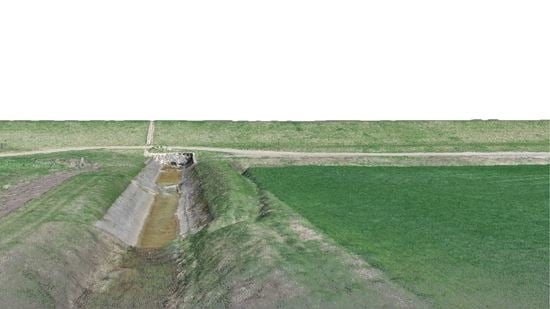
2.1. Study Area

The survey experiment was executed on an earthen dam next to a village called Pișchia, 20 km northwest from Timisoara in Western Romania. The Pișchia dam, managed by the National Water Administration, has a volume of approximately 500,000 m3, which is used to supply drinking water and for recreational activities (e.g., fishing). It has a trapezoidal cross-section with a side slope of 1:3 and a maximum elevation of about 10 m. The surrounding area is characterized by agricultural land with gentle slopes (Figure 2).

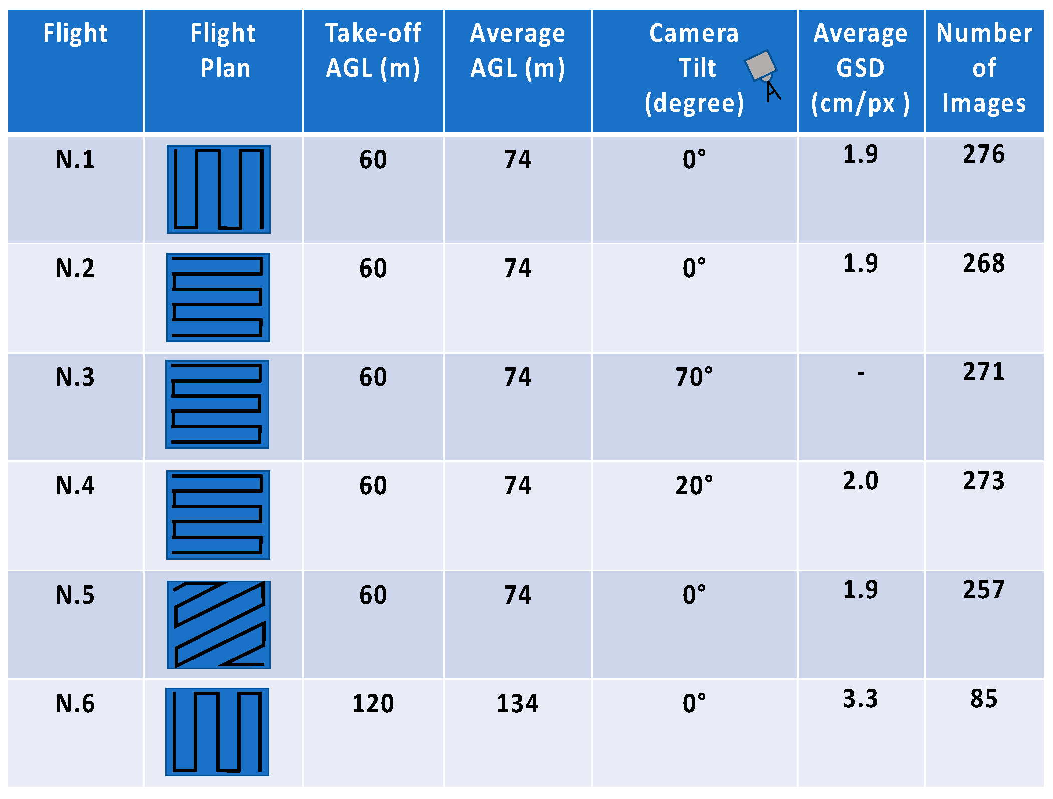
2.2. Primary Data Collection

All flights were performed with DJI Phantom 4 Pro quadcopter (DJI, Shenzhen, China), featuring a gimbaled 1-inch 20-megapixel CMOS sensor with a mechanical shutter. The focal length of the lens was 24 mm (full-frame equivalent). The data were stored in 24 bit JPG format, and the pixel size was 2.41 μm. The camera sensitivity was set to ISO100 for all images, with the aperture ranging from 4 to 5.6 and the shutter times ranging between 1/120 and 1/500 s. All images were georeferenced with the on-board GPS. The WGS84 coordinates were stored in JPG EXIF. Mission planning was executed in Pix4Dcapture, which enabled control of the camera tilt. All six flights were performed on 4 April 2018, between 10:00 a.m. and 12:50 p.m. UTC. Flight missions were planned with a side overlap of 60% and a front overlap of 80%.
In order to explore the impact of mission planning on the overall accuracy of UAS-derived DSM, different flight plans were created, with changing flight trajectories, camera tilt, and the elevation of the flight. Several characteristics of the six flights are summarized in Figure 3, whereas other parameters, such as camera settings and additional mission flight settings (e.g., overlap), were kept constant. The reference elevation refers to the take-off location, which was about 14 m above the average elevation of the surface. Some examples of the images obtained by different configurations are shown in Figure 4, where an area from the central part of the dam is reproduced. From these images, the outlet tower and the spillway of the dam can be recognized.
Flights were planned to cover an area of approximately 100 × 270 m (about 2.7 ha) and the extent is highlighted in Figure 2B (see red line boundaries). In the same figure, we report the UAS-derived DSM of the area.
For the aim of the present study, only a portion of the dam was studied using about 16 GCPs distributed along the main structure of the dam and in the adjacent agricultural area. They were placed along five longitudinal alignments, trying to measure the full range of elevation changes. The maximum vertical variation of the GCP positions was about 10.6 m.
The GCP positions were determined using the Leica 1200 system of RTK (Real-Time Kinematic) GNSS (Global Navigation Satellite System) rover (Leica Geosystems AG, Heerbrugg, Switzerland) and a precise Leica 1201 Total Station to achieve a precision better than 3 mm for all GCPs. To determine a geodetic base, corrections were acquired from the Romanian Position Determination System (ROMPOS) network of GNSS permanent stations. The study area where determinations were realized is located at a distance of 18.5 km from the TIM1 reference station (http://rompos.ro/index.php/en/).

2.3. Data Processing

Images retrieved by each flight were processed using Agisoft PhotoScan v.1.4.3 to derive a 3D model of the area. The same workflow was repeated each time while keeping the software settings constant, and following a sequence of commands: (1) photo alignment with high accuracy, (2) optimizing alignment, (3) dense cloud building with high quality aggressive depth filtering, (4) mesh building using a dense cloud, (5) texture building with the default blending mode, (6) tiled model building, (7) DSM building using the default settings, and (8) orthomosaic generation.
In the preliminary phase, we focused on the use of the geotagged images alone, excluding the use of GCPs. Measured GCPs were adopted as check points only to validate the results. Elaboration without the GCPs allowed us to better understand the role of the flight mode and the combination of different flights on the resulting DSM. This was completed by exploring the accuracies of DSMs obtained using imagery extracted from a single flight and from the combinations of two flights. The resulting combinations displayed wide variability in the precision of planar coordinates and elevation. This preliminary analysis allowed the identification of the best performing flight configuration and the benefits due to the use of combined flights.
To increase the quality of the 3D model, GCPs should be included in the Bundle Block Adjustment (BBA). The number and distribution of GCPs per unit area are not univocally identified in the literature, as highlighted in the introduction [28]. The number of GCPs necessary for the survey is influenced by the extent of the study area and its morphology, camera deployed, internal GPS precision, and the type of survey.
In the second phase, we analyzed the two previously identified imagery datasets in order to explore the role played by GCP density and distribution. For the second phase of the analysis, a variable number of GCPs ranging from 3 to 9 were randomly selected from the 16 control points available, while the remaining GCPs were employed as check points. This second analysis was useful for understanding the mutual benefit of flight combinations and well-designed GCP distribution. Proper use of the two settings enhances the potential of SfM-MVS algorithms in providing good quality DSMs. The comparison between single and multiple flights combined with the use of GCPs was stimulated by the need to better understand the benefits of combining multiple flights.

3. Accuracy Assessment of the 3D Models

3.1. Impact of Mission Planning on DSMs

The results of the quality assessment based on individual flights with different settings (Figure 3) and their combinations are summarized in Table 2, where we report the RMSE estimated between the DSM raster model derived by the SfM-MVS algorithms of Agisoft PhotoScan and the 16 check points distributed in the area. Table 2 provides four groups of information in the following order starting from the top: the planar error of the topographic surface, the absolute elevation, the relative elevation defined as elevation reduced by the minimum value observed among the considered validation points, and the total error due to both the planar and vertical errors. The columns and rows identify the combination of flights adopted for the analysis, including single flight configurations reported on the diagonal of each table.
These preliminary results summarize the impact of flight configuration on DSM accuracy. The relative error in the planar coordinates is significantly lower with respect to the vertical absolute error. This result can be explained by the photogrammetric principles. When the camera is not calibrated and we have weak image block geometry, reconstructing the correct height is much more difficult than reconstructing the horizontal location. The SfM-MVS estimated elevation is affected by an error of one or two orders of magnitude larger than planar georeferencing. This is a common problem of the DJI Phantom 4 that often produces a large offset between the correct height and that recorded by its GPS. Therefore, it is relatively common to apply a correction to the height values in order to remove this offset. In fact, this systematic error becomes less critical when considering the relative elevation of the surface, which is defined as the relative difference between the elevation of the point and the minimum value of the considered GCPs.
The best results in terms of planar coordinates were obtained by combining the flights N.1 and N.4, whereas the best performance in terms of relative elevation was produced by flight N.4. We observed that all combinations, including flight N.4, provided improved the accuracy of the relative elevation. Considering the total error due to both planar and vertical errors (considering the relative elevation), the best performing set of images was produced by the combination of flights N.1 and N.4. Among the tests based on a single flight, the results obtained with flight N.2 produced good results with a total error slightly higher than the best combination of two flights.
Note the low quality of the 3D models derived with images captured with a camera tilt of 70°. This camera configuration produced images with a limited amount of information that deteriorated the result in all combinations, especially for planar coordinates. In fact, it was impossible to derive a DSM using the only the data from flight N.3 alone. This survey is only beneficial in reducing the error of the absolute elevation of the DSM, but its value is limited in terms of relative elevation (see the third panel of Table 2). This result is due to the perspective distortion of the images captured with this camera tilt at this elevation (see the example given in Figure 4C).

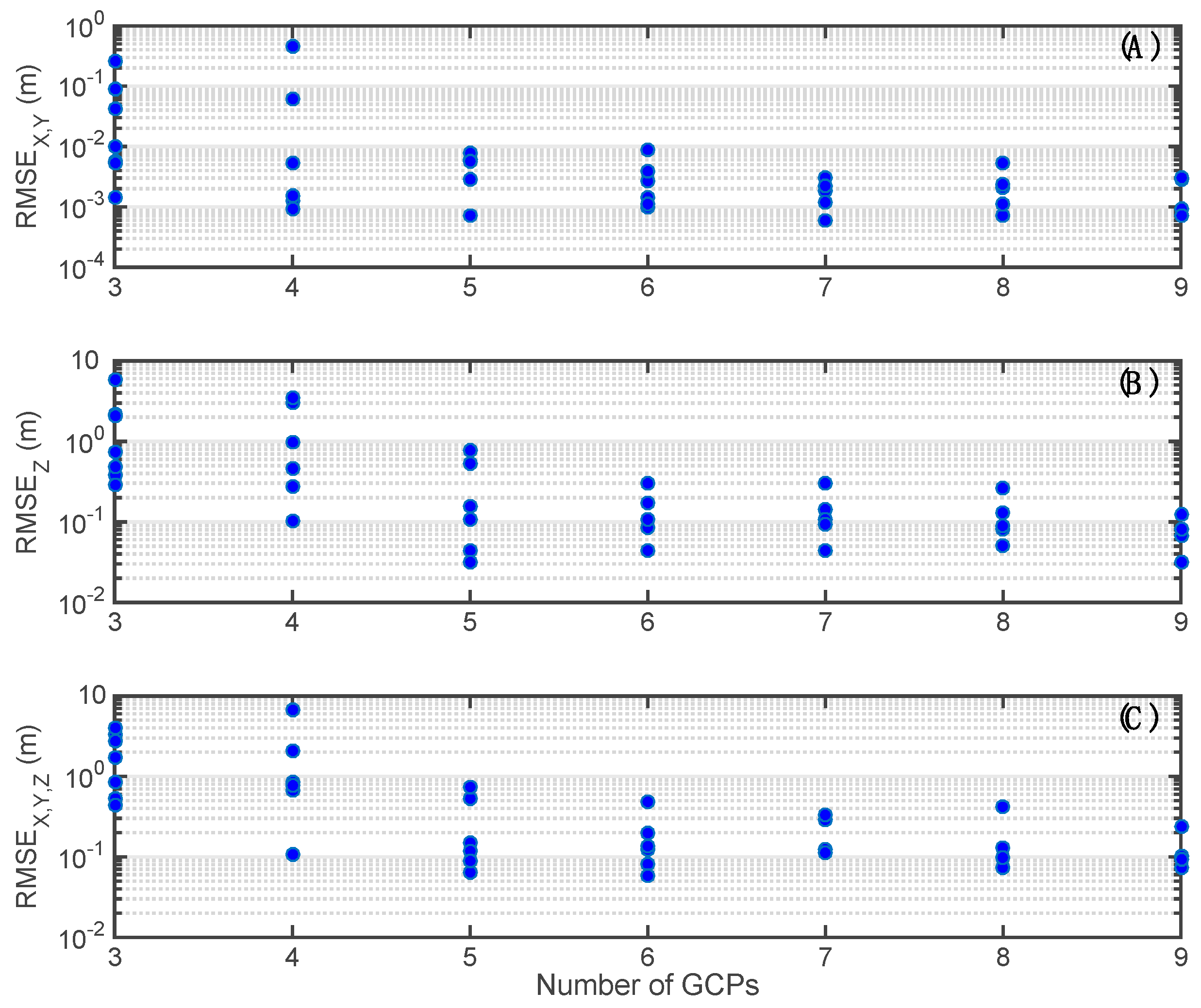
3.2. Use of GCPs in SfM-MVS Processing

The required number of GCPs was explored using several combinations of GCPs selected from the 16 check points available. We tested the planar and vertical accuracy of the 3D model generated using survey N.2 and the ensemble of images obtained from the combination of flights N.1 and N.4. Approximately 64 combinations of GCPs, with a variable number ranging from three to nine (55% of the available check points), were tested for each dataset, providing useful insight into the appropriate strategy to improve the overall accuracy of the resulting DSMs.

3.2.1. DSMs Derived from a Single Flight

In this section, we describe the accuracy assessment of the DSMs derived using the images from flight N.2. This flight was selected from those presented in the previous section because it produced the best accuracy among the single flight options explored as evidenced by the diagonal values of RMSE in Table 2.
Several DSMs were generated using different combinations of GCPs, modifying their number and relative distribution in space. The results of these analyses are summarized in Figure 5, where a sharp increase in DSM accuracy can be observed, moving from 3–4 GCPs to 5–6 GCPs. The magnitude of planar errors seems to be fairly stable after five GCPs. Vertical errors are always larger and tend to be more stable after six GCPs. The planar error reaches values of a few centimeters when adopting as few as five GCPs (Figure 5), whereas the vertical accuracy ranges from 6–74 cm for the same number of GCPs. Therefore, the total error of DSMs is mostly influenced by higher values of RMSEZ.

3.2.2. DSMs Derived from the Combination of Two Flights

By combining two flights, the general patterns were similar to those observed in the previous section. Therefore, similar considerations can be made regarding the impact of GCP number. However, some key differences were identified. Most notably, the RMSEs were generally lower when two flights of differing configurations were used, especially when more than six GCPs were adopted. Comparing the results of Figure 5 and Figure 6, the errors in terms of planar coordinates (RMSEX,Y) are comparable, but there is a critical difference in the elevation accuracy (RMSEZ). RMSEZ was less than 10 cm when more than six GCPs were adopted. This highlights the relative advantage of introducing a two-flight combination in the process because the nadir orientation provides the best configuration for the planar coordinates, whereas the 20° tilted camera increases the vertical accuracy (see Table 2 for comparison).
To emphasize the relative differences between the two configurations explored herein, the results obtained with a single flight and two flights are compared in Figure 7. This highlights the benefits of flight combinations in terms of planar (Figure 7A) and vertical (Figure 7B) accuracy. The two configurations display minimal differences in terms of planar accuracy, while the vertical precision results are significantly improved when two flights are adopted. The DSMs obtained using the best combination of two flights produced a vertical accuracy of about 3.5 cm if six or more GCPs were used. The results appeared to be relatively stable with more than six GCPs.

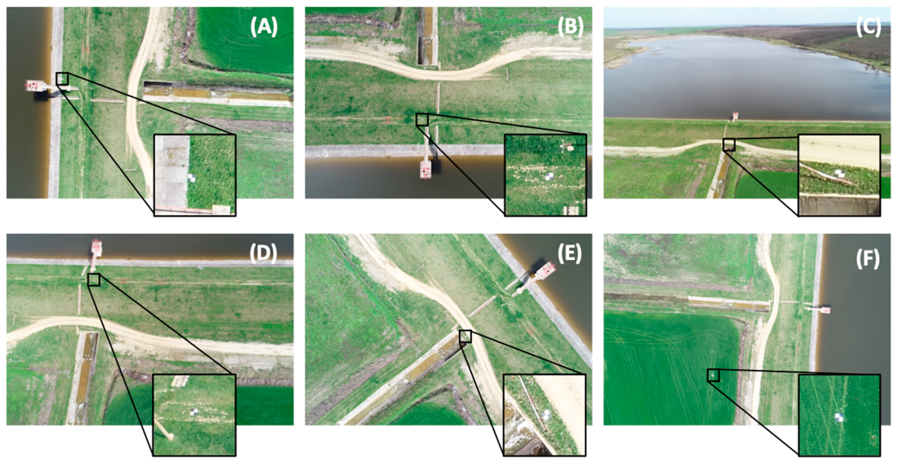
3.2.3. Spatial Distribution of GCPs

The spatial distribution of GCPs strongly controls the DSM accuracy. Its influence was explored considering the relative changes in the planar and vertical RMSE as a function of the mean relative to the distance between the GCPs on the plane (Figure 8A,C) and in elevation (Figure 8B,D). Notably, the mean distance is a measure of dispersion and, therefore, its increase means an increase in the spatial dispersion of the points.
We analyzed the two cases under investigation: (1) the single flight (Figure 8A,B) and (2) the combination of two flights (Figure 8C,D). The comparison of the performance associated with different numbers of GCPs adopted for the elaboration revealed significantly different RMSE values. Therefore, we used the relative change of RMSE, which is computed with respect to the average RMSE estimated for a subset of data associated with a given number of GCPs, in order to remove the effect of differences in GCP number. Relative changes in the planar RMSE show a clear decrease with an increasing mean distance, whereas vertical errors seem to be less influenced by the vertical spread of GCPs, especially in the case of two flights.
Therefore, the spatial distribution of GCPs strongly controls the planar and vertical DSM accuracy. We observed that the accuracy increases with mean GCP distance especially when analysis is based on a single flight (see Figure 8A,B). This suggests that GCPs should be spread in space as much as possible to cover the entire range of variability in elevation and fulfill the extent of the area. These results corroborate the findings of James and Robson [31] and Smith and Vericat [13] in suggesting that the distribution of GCPs is both across and to the edges of the target area. Therefore, the GCP distribution could have been improved including four GCPs at the corners of the study area.
The impact of the spatial distribution of GCPs seems to be less relevant when a combination of two flights including a tilted camera is adopted. In this case, vertical accuracy is not influenced by the vertical spread of GCPs. In practice, the regular spread of GCPs is not always possible due to site inaccessibility, forest cover, etc., emphasizing the value of our findings in showing how a combination of two flights can improve vertical accuracy.

4. Discussion

UAS-derived 3D models provide a new strategy for monitoring land surfaces with an extremely high level of detail. The literature offers a wide range of applications for the operational use of UASs for 3D model reconstruction based on SfM-MVS algorithms, offering different strategies aimed at minimizing the errors of these 3D models. A review of these studies enabled the identification of the control exerted by GCP density on the planar and vertical accuracy of UAS-derived DSMs. The planar accuracy of SfM-MVS outputs is generally higher than the vertical accuracy. Therefore, the number of GCPs needed to produce stable results is generally lower for planar coordinates. On average, five GCPs/ha are enough to produce a good performance on the plane, but doubled density is needed for elevation (Figure 1). The final result is highly influenced by other factors such as flight pattern and configuration, camera quality, and local morphological complexity.
In our analysis, we focused on 3D model optimization exploiting the combination of different flight configurations and the optimal GCP design. For this reason, we explored the impact of: (1) the combined use of images obtained from different flight patterns and configurations, and (2) the use of a variable number of GCPs. Both approaches are already used in a practical application without clear identification of the benefits associated with combining images acquired using different flight plans and camera settings, or the quantification of the impact of such choices. The optimum density and distribution of GCPs remain poorly understood.
According to our results, mission planning is a critical preliminary step that may significantly affect the final results. In certain circumstances, a well-defined single flight may be sufficient to produce adequate quality for the overall survey. The combination of flights with differing configurations can retrieve information from different viewpoints and angles that can increase the resulting accuracy. Given the optical nature of SfM-MVS algorithms, the challenge is then to maximize the number of observations of each individual point retrieved across the area of interest. The use of a tilted camera may be beneficial in order to improve the robustness of the geometrical model, thereby increasing the number of tie points describing inclined surfaces. The tilt of the camera should be defined according to both the local morphology and the resolution required. For the studied case, characterized by a trapezoidal earthen dam with an elevation of about 10 m and gentle slopes with elevation changes of 15 m, a tilt of 20° combined with a 0° flight provided the best results. This result can be justified by examining the results reported on the diagonal of Table 2. The accuracy of planar coordinates was generally higher when using a nadir camera setting with lower flight altitude, but the vertical error was always lower for the flight with a 20° tilted camera. Therefore, a combination of two flights tends to optimize both characteristics of DSMs.
The flights operated on two orthogonal routes provided additional benefits to the description of the area, allowing a relevant reduction of error (for comparison, see the results of the combination 1–2). Comparing the accuracy of different DSMs obtained with a single flight or a combination of flights, the flight combination and tilted camera significantly increased the vertical accuracy, clearly benefiting to the process of DSM construction.
The error magnitude is also influenced by the flight altitude that controls the image resolution. The use of multiple flights at different flight altitudes is a common practice to improve survey accuracy in aerial photogrammetry [32]. We observed a beneficial effect on the relative elevation accuracy of DSM, but such improvement is probably also influenced by the lower resolution of the images and is less effective in general than the use of a 20° tilted camera. In the literature, contrasting results on the relative impact of the flight altitude have been reported. For example, Gómez-Candón et al. [23] showed a weak relationship of RMSE with flight height.
The orthorectification of images is traditionally performed using GCPs. Other options should also be considered, such as investing in carrier-phase GPS receivers and processing workflow that can reduce the amount of fieldwork needed in terms of GCP collection [33], which is especially useful if monitoring larger areas.
Our results show that, with an increasing number of GCPs, the quality of the 3D model increases. With five GCPs, a planar RMSE of less than one centimeter (about 0.2 cm) was reached. High vertical accuracy requires significant additional effort. Our dataset confirms the need to increase the number of GCPs to achieve a stable result in terms of the vertical RMSE. Even if the maximum number of nine GCPs was adopted, the obtained vertical accuracy was still one order of magnitude larger than the planar accuracy. Only adopting a combination of flights significantly in the vertical accuracy of the DSM, reaching a precision of about 4 cm after more than seven GCPs were adopted.
High planar accuracy can be obtained with a relatively small number of GCPs well spread in space, whereas vertical accuracy requires a larger number of GCPs and is less sensitive to their relative distribution in space. As shown in our study, the vertical accuracy, a critical variable in several studies, can be significantly improved using a combination of flights, including the use of a tilted camera, thereby reducing the laborious and complicated collection of GCPs. Notably, this method is the most efficient approach to reduce vertical error among the many methods explored herein.
The proposed study is based on low-cost technology that is commonly used, but there is a tendency toward the inclusion of more accurate positioning systems in UASs that will dramatically reduce the need for ground operations. These new systems are still expensive, but will certainly become more affordable shortly. For instance, Gerke and Przybilla [34] explored the impact of onboard RTK-GNSS on DSM accuracy and observed a significant enhancement in absolute image orientation accuracy with this option.

5. Conclusions

In this paper, we provided recommendations for UAS-surveys aimed at the derivation of 3D surface models. Exploiting the available literature on this topic and our field experiences, a number of suggestions are put forward:
(1)
UAS-derived orthomosaics can produce a planar accuracy of a few centimeters, whereas the vertical accuracy of DSMs is always lower. This is likely due to the fact that most UASs adopt a camera in a zenithal position that provides a more accurate description of planar features. Vertical measurements are generally more complex, but also critical for studies of change detection.
(2)
The flight plan and camera configuration may significantly impact the overall quality of the resulting DSM. Therefore, it should be planned thoroughly to produce the best depiction of the entire area. For instance, a transversal survey with respect to a given structure provides better description and quality of the resulting 3D surface.
(3)
The use of a tilted camera can improve the amount of information (retrieved number of points) for inclined surfaces, providing higher DSM elevation accuracy. The tilted camera images increase the robustness of the geometrical model, providing also a possible strategy to reduce the total number of GCPs adopted over a given area. This can be beneficial especially in inaccessible areas.
(4)
The combination of several flights may be extremely beneficial for DSM accuracy. This improves the overall quality of the results, exploiting information redundancy derived by different flight plans and camera configurations.
(5)
The planar and vertical accuracies can be improved by increasing the number of GCPs and their relative distances. It is therefore convenient to evenly spread GCPs in space. In many cases, such ideal settings are not possible and a combination of flights, that include the use of a tilted camera, can be used to reduce sensitivity to this parameter in the final vertical accuracy of the DSMs.
Our described experiment cannot be considered exhaustive; however, it provides insights into the problems discussed and can serve as a guideline for future applications. Extending the analysis to new case studies and landscape morphologies is highly desirable to provide clear and more detailed guidelines for UAS applications to considering other factors influencing DSM accuracy, such as site area and morphology, sensor, and internal GPS precision. The outcomes of the presented research lead to a number of useful results applicable to UAS applications in different conditions. There is no simple solution for the optimal number of GCPs, but our analysis helps with understanding some general concepts. To conclude, the flight should be planned carefully in order to optimize the amount of information retrieved by the camera deployed, and combined flight settings can significantly improve the overall quality of the 3D models, even for the most critical dimension—the vertical accuracy.
The present manuscript represents a preliminary step for the definition of guidelines for UAS-derived DSMs. Nevertheless, the procedure is influenced by several additional factors that have not been taken into consideration in the present study. Therefore, we plan to extend our study considering different morphologies, SfM-algorithms and devices in future activities.

Author Contributions

S.M. conceived and coordinated the work and the writing; P.D., S.H., and J.J.A.J. supported the field activities and interpretation of the results; P.V. performed the numerical analysis; J.M. and M.P. supported the interpretation of the results and the writing.

Funding

This research was funded by the COST Action CA16219 “HARMONIOUS—Harmonization of UAS techniques for agricultural and natural ecosystems monitoring”. JM was supported by LTC18007 and RVO 67985939. PD was supported by LTC18007 and by the MEYS under the National Sustainability Programme I (Project LO1202).

Conflicts of Interest

The authors declare no conflict of interest.

References

  1. Cook, S.J.; Clarke, L.E.; Nield, J.M. Geomorphological Techniques (Online Edition); British Society for Geomorphology: London, UK, 2012. [Google Scholar]
  2. Kraus, K.; Waldhausl, P. Photogrammetry, Volume 1: Fundamentals and Standard Processes; Ferd. Dümmlers Verlog: Bonn, Germany, 1993. [Google Scholar]
  3. Krauss, K.; Jansa, J.; Kager, H. Photogrammetry, Volume 2: Advanced Methods and Applications; Ferd. Dümmlers Verlog: Bonn, Germany, 1997. [Google Scholar]
  4. Luhmann, T.; Robson, S.; Kyle, S.A.; Harley, I.A. Close Range Photogrammetry: Principles, Techniques and Applications; Whittles: Dunbeath, UK, 2006. [Google Scholar]
  5. Mikhail, E.M.; Bethel, J.S.; McGlone, J.C. Introduction to Modern Photogrammetry; John Wiley & Sons: Hoboken, NJ, USA, 2001. [Google Scholar]
  6. Manfreda, S.; McCabe, M.F.; Miller, P.; Lucas, R.; Pajuelo Madrigal, V.; Mallinis, G.; Ben Dor, E.; Helman, D.; Estes, L.; Ciraolo, G.; et al. On the Use of Unmanned Aerial Systems for Environmental Monitoring. Remote Sens. 2018, 10, 641. [Google Scholar] [CrossRef]
  7. Nex, F.; Remondino, F. UAV for 3D mapping applications: A review. Appl. Geomat. 2014, 6, 1–15. [Google Scholar] [CrossRef]
  8. Westoby, M.J.; Brasington, J.; Glasser, N.F.; Hambrey, M.J.; Reynolds, J.M. ‘Structure-from-Motion’ photogrammetry: A low-cost, effective tool for geoscience applications. Geomorphology 2012, 179, 300–314. [Google Scholar] [CrossRef] [Green Version]
  9. Colomina, I.; Molina, P. Unmanned aerial systems for photogrammetry and remote sensing: A review. ISPRS J. Photogramm. Remote Sens. 2014, 92, 79–97. [Google Scholar] [CrossRef] [Green Version]
  10. Whitehead, K.; Hugenholtz, C.H.; Myshak, S.; Brown, O.; LeClair, A.; Tamminga, A.; Barchyn, T.E.; Moorman, B.; Eaton, B. Remote sensing of the environment with small unmanned aircraft systems (UASs), part 2: Scientific and commercial applications. J. Unmanned Veh. Syst. 2014, 2, 86–102. [Google Scholar] [CrossRef]
  11. Lucieer, A.; Jong, S.M.D.; Turner, D. Mapping landslide displacements using Structure from Motion (SfM) and image correlation of multi-temporal UAV photography. Progr. Phys. Geogr. 2014, 38, 97–116. [Google Scholar] [CrossRef]
  12. Clapuyt, F.; Vanacker, V.; Van Oost, K. Reproducibility of UAV-based earth topography reconstructions based on Structure-from-Motion algorithms. Geomorphology 2016, 260, 4–15. [Google Scholar] [CrossRef]
  13. Smith, M.W.; Vericat, D. From experimental plots to experimental landscapes: Topography, erosion and deposition in sub-humid badlands from structure-from-motion photogrammetry. Earth Surf. Process. Landf. 2015, 40, 1656–1671. [Google Scholar] [CrossRef]
  14. James, M.R.; Robson, S.; d’Oleire-Oltmanns, S.; Niethammer, U. Optimising UAV topographic surveys processed with structure-from-motion: Ground control quality, quantity and bundle adjustment. Geomorphology 2017, 280, 51–66. [Google Scholar] [CrossRef]
  15. Carrivick, J.L.; Smith, M.W.; Quincey, D.J. Structure from Motion in the Geosciences; John Wiley & Sons: Hoboken, NJ, USA, 2016. [Google Scholar]
  16. Ridolfi, E.; Buffi, G.; Venturi, S.; Manciola, P. Accuracy Analysis of a Dam Model from Drone Surveys. Sensors 2017, 17, 1777. [Google Scholar] [CrossRef]
  17. Singh, K.K.; Frazier, A.E. A meta-analysis and review of unmanned aircraft system (UAS) imagery for terrestrial applications. Int. J. Remote Sens. 2018. [Google Scholar] [CrossRef]
  18. Rock, G.; Ries, J.B.; Udelhoven, T. Sensitivity analysis of UAV-photogrammetry for creating digital elevation models (DEM). In Proceedings of the Conference on Unmanned Aerial Vehicle in Geomatics, Zurich, Switzerland, 14–16 September 2011. [Google Scholar]
  19. Tahar, K.N. An evaluation on different number of ground control points in unmanned aerial vehicle photogrammetric block. Int. Arch. Photogramm. Remote Sens. Spat. Inf. Sci. 2013, 40, 93–98. [Google Scholar] [CrossRef]
  20. Mancini, F.; Dubbini, M.; Gattelli, M.; Stecchi, F.; Fabbri, S.; Gabbianelli, G. Using unmanned aerial vehicles (UAV) for high-resolution reconstruction of topography: The structure from motion approach on coastal environments. Remote Sens. 2013, 5, 6880–6898. [Google Scholar] [CrossRef]
  21. Hugenholtz, C.H.; Whitehead, K.; Brown, O.W.; Barchyn, T.E.; Moorman, B.J.; LeClair, A.; Riddell, K.; Hamilton, T. Geomorphological mapping with a small unmanned aircraft system (sUAS): Feature detection and accuracy assessment of a photogrammetrically-derived digital terrain model. Geomorphology 2013, 194, 16–24. [Google Scholar] [CrossRef] [Green Version]
  22. Cryderman, C.; Mah, S.B.; Shufletoski, A. Evaluation of UAV photogrammetric accuracy for mapping and earthworks computations. Geomatica 2014, 68, 309–317. [Google Scholar] [CrossRef]
  23. Gómez-Candón, D.; De Castro, A.I.; López-Granados, F. Assessing the accuracy of mosaics from unmanned aerial vehicle (UAV) imagery for precision agriculture purposes in wheat. Precis. Agric. 2014, 15, 44–56. [Google Scholar] [CrossRef]
  24. Uysal, M.; Toprak, A.S.; Polat, N. DEM generation with UAV Photogrammetry and accuracy analysis in Sahitler hill. Measurement 2015, 73, 539–543. [Google Scholar] [CrossRef]
  25. Küng, O.; Strecha, C.; Beyeler, A.; Zufferey, J.C.; Floreano, D.; Fua, P.; Gervaix, F. The accuracy of automatic photogrammetric techniques on ultra-light UAV imagery. Int. Arch. Photogramm. Remote Sens. Spat. Inf. Sci. 2011, 125–130. [Google Scholar] [CrossRef]
  26. Agüera-Vega, F.; Carvajal-Ramírez, F.; Martínez-Carricondo, P. Assessment of photogrammetric mapping accuracy based on variation ground control points number using unmanned aerial vehicle. Measurement 2017, 98, 221–227. [Google Scholar] [CrossRef]
  27. Koci, J.; Jarihani, B.; Leon, J.X.; Sidle, R.C.; Wilkinson, S.N.; Bartley, R. Assessment of UAV and ground-based Structure from Motion with multi-view stereo photogrammetry in a gullied savanna catchment. ISPRS Int. Geo-Inf. 2017, 6, 328. [Google Scholar] [CrossRef]
  28. Oniga, V.-E.; Breaban, A.-I.; Statescu, F. Determining the Optimum Number of Ground Control Points for Obtaining High Precision Results Based on UAS Images. Proceedings 2018, 2, 352. [Google Scholar] [CrossRef]
  29. Tonkin, T.N.; Midgley, N.G. Ground-Control Networks for Image Based Surface Reconstruction: An Investigation of Optimum Survey Designs Using UAV Derived Imagery and Structure-from-Motion Photogrammetry. Remote Sens. 2016, 8, 786. [Google Scholar] [CrossRef]
  30. Gindraux, S.; Boesch, R.; Farinotti, D. Accuracy Assessment of Digital Surface Models from Unmanned Aerial Vehicles’ Imagery on Glaciers. Remote Sens. 2017, 9, 186. [Google Scholar] [CrossRef]
  31. James, M.R.; Robson, S. Straightforward reconstruction of 3D surfaces and topography with a camera: Accuracy and geoscience application. J. Geophys. Res. Earth Surf. 2012, 117, F03017. [Google Scholar] [CrossRef]
  32. Pepe, M.; Fregonese, L.; Scaioni, M. Planning airborne photogrammetry and remote-sensing missions with modern platforms and sensors. Eur. J. Remote Sens. 2018, 51, 412–436. [Google Scholar] [CrossRef]
  33. Müllerová, J.; Bartaloš, T.; Brůna, J.; Dvořák, P.; Vítková, M. Unmanned aircraft in nature conservation—An example from plant invasions. Int. J. Remote Sens. 2017, 38, 2177–2198. [Google Scholar] [CrossRef]
  34. Gerke, M.; Przybilla, H.-J. Accuracy analysis of photogrammetric UAV image blocks: Influence of onboard RTK-GNSS and cross flight patterns. Photogramm.-Fernerkund.-Geoinf. 2016, 2016, 17–30. [Google Scholar] [CrossRef]
Figure 1. Digital surface models (DSMs) accuracy in terms of planar and vertical root mean squared error (RMSE) as a function of the ground control points (GCPs) density (data extracted from the literature reported in Table 1).
Drones 03 00015 g001
Figure 2. (A) Position of the study area within Europe (45.927N, 21.335E). (B) Description of the study area and distribution of the GCPs. (C) Unmanned aerial system (UAS)-derived DSM of the area.
Drones 03 00015 g002
Figure 3. Characteristics of the different surveys carried out during the experiment: flight pattern, above ground level (AGL) at the take-off, average AGL, camera tilt, average ground sample distance (GSD), and number of images.
Drones 03 00015 g003
Figure 4. Images of the central part of the dam body acquired during flight (A) N.1, (B) N.2, (C) N.3, (D) N.4, (E) N.5, and (F) N.6. In each image, a GCP is emphasized and magnified.
Drones 03 00015 g004
Figure 5. RMSE of the DSM raster model as a function of the number of GCPs adopted for the elaboration: (A) RMSE in planar coordinates, (B) RMSE in relative elevation, and (C) RMSE in X, Y, and Z obtained for the flight N.2.
Drones 03 00015 g005
Figure 6. RMSE of the 3D model as a function of the number of GCPs adopted in the model run. (A) The RMSE in planar coordinates, (B) the RMSE in relative elevation, and (C) the RMSE in X, Y, and Z directions for the combination of flights N.1 and N.4.
Drones 03 00015 g006
Figure 7. Comparison of results obtained changing the number of GCPs and adopting a single flight or a two-flight combination dataset on the (A) plane and (B) z-axis.
Drones 03 00015 g007
Figure 8. Relative change in RMSE with respect to the mean value associated with a given number of GCPs as a function of the mean distance between GCPs obtained for (A,B) flight N.2 and (C,D) the combination of flights N.1 and N.4. In each panel, linear regression is reported to provide a measure of the existing dependence between the two variables.
Drones 03 00015 g008
Table 1. Precision of digital surface models (DSMs) created using a variable number of ground control points (GCPs).
ReferenceArea
(ha)
Number
of GCPs
AGL
(m)
RMSEX,Y
(cm)
RMSEZ
(cm)
RMSE
Total (cm)
Rock et al. [18]N/A104250–550N/A5.5N/A
Tahar [19]1508–9N/A50.078.0N/A
Mancini et al. [20]2.7518400.810.0N/A
Hugenholtz et al. [21]4.5282001829N/A
Lucieer et al. [11]0.7539N/A7.46.2N/A
Cryderman et al. [22]7.12111183.33.14.6
Gómez–Candón et al. [23]1.011–4530–100N/AN/A0.29–0.12
Uysal et al. [24]5.02760N/A6.62N/A
Kung et al. [25]210.01926238107125
Agüera-Vega et al. [26]17.644–15–201207–4.5–1.733–5.8–4.7N/A
Koci et al. [27]41–45–726–7100N/A30.9–68.7–95.9N/A
James et al. [14]7.54–271004.9N/A1.6
Oniga et al. [28]1.03–4028–354.5–8.96.6–4.07.4–7.9
Table 2. Root Mean Square Error (RMSE) estimated on 16 GCPs for planar coordinates, absolute elevation, relative elevation defined as elevation reduced by the minimum value observed among the considered validation points, and the sum of the planar and vertical error obtained using different images taken from different flight combinations (for description, see Figure 3). The values written in bold represent the best performing configuration for each specific sub-group.
Planar Coordinates—RMSEX,Y (m)
FlightN.1N.2N.3N.4N.5N.6
N.14.47
N.22.392.03
N.3136.051497.25-
N.41.643.083835.207.75
N.52.091.9515,042.568.057.15
N.63.063.351750.118.636.9419.70
Elevation—RMSEZ (m)
FlightN.1N.2N.3N.4N.5N.6
N.182.90
N.281.1878.72
N.380.3256.94-
N.479.2176.9415.5175.02
N.577.9077.867.7073.3571.86
N.678.7975.4820.2572.8570.2759.75
Relative Elevation—RMSEZ (m)
FlightN.1N.2N.3N.4N.5N.6
N.11.06
N.20.390.37
N.33.7419.55-
N.40.550.425.880.11
N.50.390.258.000.470.26
N.60.220.9413.850.800.403.44
Planar and vertical—RMSE (m)
FlightN.1N.2N.3N.4N.5N.6
N.14.59
N.22.422.06 Performances
N.3136.101497.38- Good
N.41.733.113835.207.75 Medium
N.52.131.9715,042.568.067.15 Low
N.63.073.481750.168.676.9520.00

