Acoustic Detection of a Fixed-Wing UAV

Abstract

The following paper presents results obtained from experiments conducted to investigate the viability of acoustic sensing to form the basis of a non-cooperative aircraft collision avoidance system. An unmanned aerial vehicle (UAV) fitted with two microphones was flown in the vicinity of another airborne UAV to determine the maximum distance at which the intruding aircraft could be detected. A two-dimensional analytical model to approximate the minimum detection distance required to facilitate an avoidance maneuver for a given spatial configuration is presented. A method to increase detection distances by exploiting the harmonic nature of acoustic signals generated by propeller-driven aircraft is also presented. The method significantly increases the detection distances compared to the commonly used incoherent spectral mean. It was found that a small gasoline-powered UAV could be detected at distances up to 678 m, which is more than double the minimum required to avoid a head-on collision.

1. Introduction

Unmanned aerial vehicles (UAVs) are a rapidly advancing technology with many applications in the private, commercial, and government sectors. Currently, however, no safeguards exist to facilitate the safe operation of these devices in populated uncontrolled airspace without posing potential hazards to other manned or unmanned aircraft. Conventional anti-collision systems are only required for passenger aircraft greater than 5700 kg, and must be present on both to enable operation [1]. Since autonomous UAVs do not meet these requirements and do not have the benefit of an onboard pilot, a non-cooperative system must be established to facilitate the detection and subsequent avoidance of other approaching aircraft. It is believed that acoustic sensing may be used to serve such a purpose.

Acoustic sensing is a passive technology that involves the detection of acoustic wave energy produced by some oscillating body. The most common form involves using sensors known as microphones that detect pressure fluctuations created during wave transmission. Acoustic sensing has many potential benefits over the more traditional non-cooperative technologies such as electro-optic (EO), infrared (IR), and radar. Since sensors are typically omnidirectional, complete spherical sensing coverage can be achieved. This is a very important feature as the bulk of midair collisions take place from behind, the side, above, or below; locations that would typically fall outside the field of view for most other sensing technologies [2]. Sensing systems are typically very small and lightweight since they consist of only a few microphones and a data recording/processing unit. Data acquisition and processing requirements are also much less than that of EO or IR due to decreased sensor data rates. By simultaneously using a number of spatially separated microphones in an array configuration, the detection, localization, and tracking of an acoustic source such as an aircraft can be achieved [3,4,5,6,7,8]. In some instances, analyzing the Doppler-induced frequency shift of the source signal over a period of time may also allow one to determine the velocity and heading of the sound source [8,9,10,11,12].

The general use of acoustic sensing to detect, localize, and track moving targets has been well studied and documented in the literature [3,4,5,6,7,8]. However, there have been very few accounts of using this technology for UAV sense-and-avoid (SAA) purposes. There have been no reports of air-to-air detection and localization of another aircraft from either a fixed-wing or rotary-wing UAV. Work in this area has involved either the detection of airborne UAVs from stationary platforms such as ground-based microphone arrays or tethered aerial balloons [2,10,13,14,15,16], simulating a UAV-based detection system [2,17,18,19], detecting ground-based impulse sources from fixed-wing UAVs, [20,21], or localizing continuous ground-based sources from stationary low-altitude rotary-wing UAVs [22,23].

Ferguson [20] utilized a small UAV (Aerosonde) fitted with two microphones to detect and localize acoustic impulses from a propane cannon located on the ground. Detection distances of up to 300 m were said to have been achieved with a localization bearing angle error of 3°; although, evidence for these claims was not clearly presented. Robertson [21] also conducted experiments where a ground-based propane cannon was detected and localized from a small UAV fitted with four microphones. Detection distances of up to 180 m were claimed with an average localization error of 8°. Ohata used a multirotor fitted with a large number of MEMS microphones to detect and localize an acoustic source located on the ground while hovering at altitudes less than 5 m [22,23]. Although a high localization accuracy was achieved, detection distances were far too low to constitute any form of practical anti-collision system. Scientific Applications and Research Associates Inc. (SARA) has developed a compact acoustic sensor system known as the Passive Acoustic Non-Cooperative Collision Alert System (PANCAS) for use on small UAVs [24]. It has been integrated on a number of small gasoline-powered UAVs and supposedly obtained detection ranges of up to 2 km [25]. However, there are currently no accounts published in the scientific literature regarding this technology to support this particular claim. One publication did, however, briefly indicate that the system was capable of detecting a shockwave emitted from a ground-based propane cannon from a distance of approximately 180 m via a fixed-wing UAV [21]. Finally, Harvey showed that a ground-based loudspeaker emitting a 119 dBc audio recording of a small gasoline-powered UAV should be detectable at distances up to 1 km by a fixed-wing UAV fitted with four microphones [26].

Although acoustic sensing is a relatively new idea in the context of collision avoidance technologies, it is evident that results obtained from studies conducted thus far appear promising. However, significant work is still required to fully evaluate the capabilities and limitations of the technology. Thus, the purpose of the following paper is to provide results from experiments conducted to further investigate the use of acoustic sensing as a collision avoidance technology. These results consist of determining the maximum distance at which a gasoline-powered fixed-wing UAV can be detected by an electric powered fixed-wing UAV fitted with microphones. It should be noted that details regarding localization and tracking of the intruding aircraft are not presented in the current paper due to the increased length that it would entail and will be presented in a future paper instead. In addition to experimental results, a method to enhance the detection of harmonic signals such as those generated by propeller-driven aircraft is also provided.

2. Experimental Methods

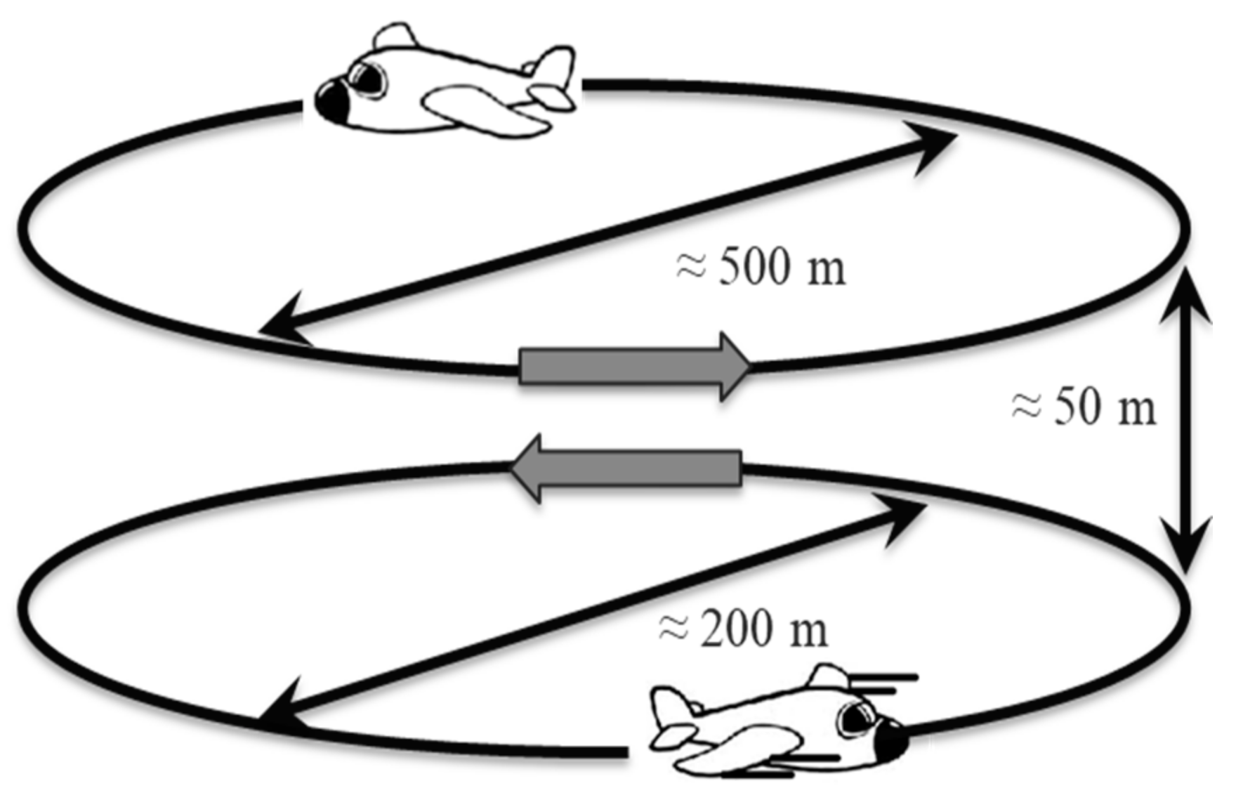
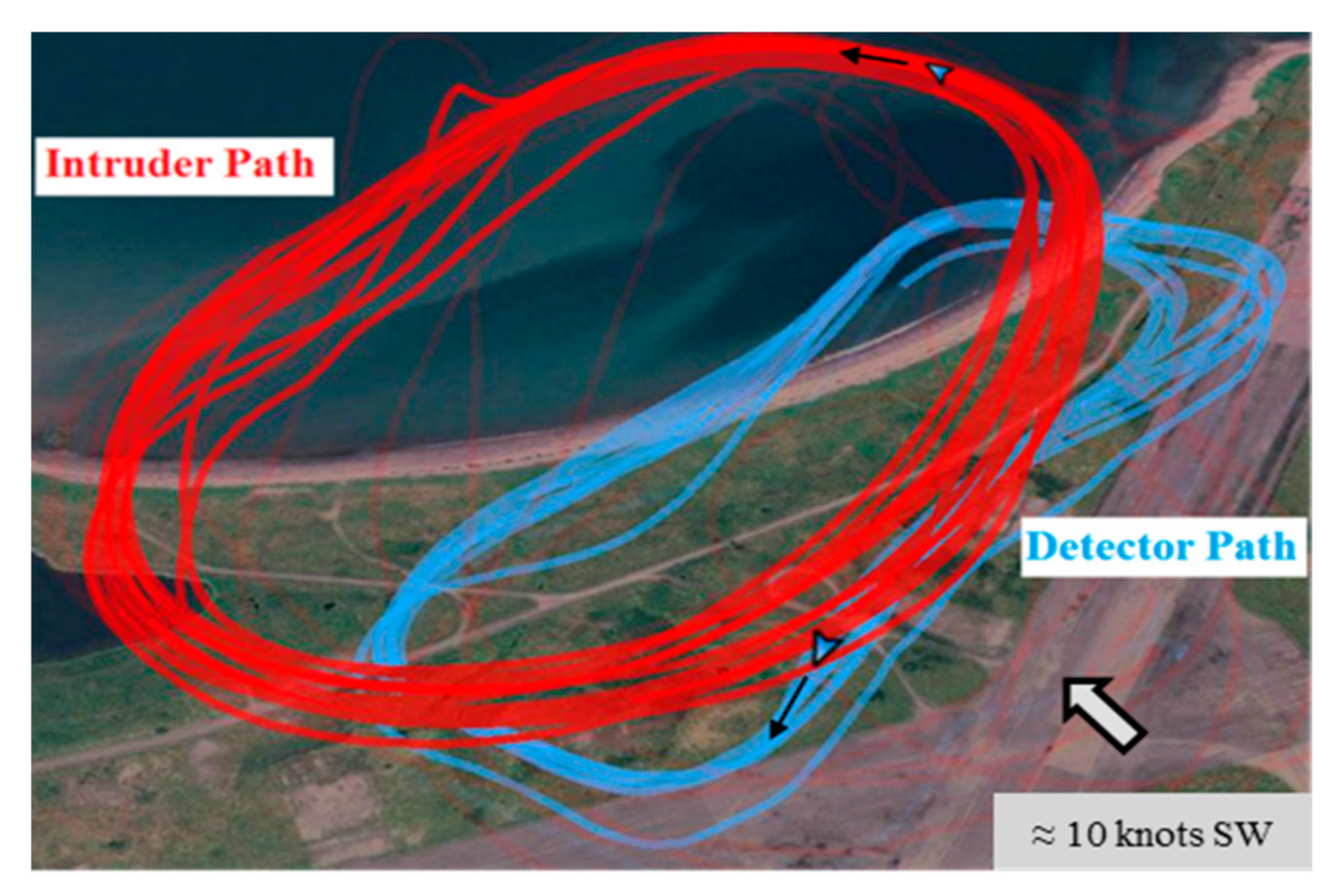
The conducted experiment involved flying two aircraft (sensing and intruding) in circuit formation with opposing flight paths to facilitate close mid-air encounters. The aircraft were assigned different altitudes and circuit radii to avoid any actual mid-air collision from taking place. The intruder was given an altitude of 150 m with a circuit radius of approximately 500 m, while the detecting aircraft was given an altitude and circuit radius of 100 m and 200 m, respectively. Figure 1 and Figure 2 provide a depiction of the experimental setup and a Google Earth image of the aircraft GPS tracks. The total duration of the experiment was 830 s and consisted of 25 close encounters.

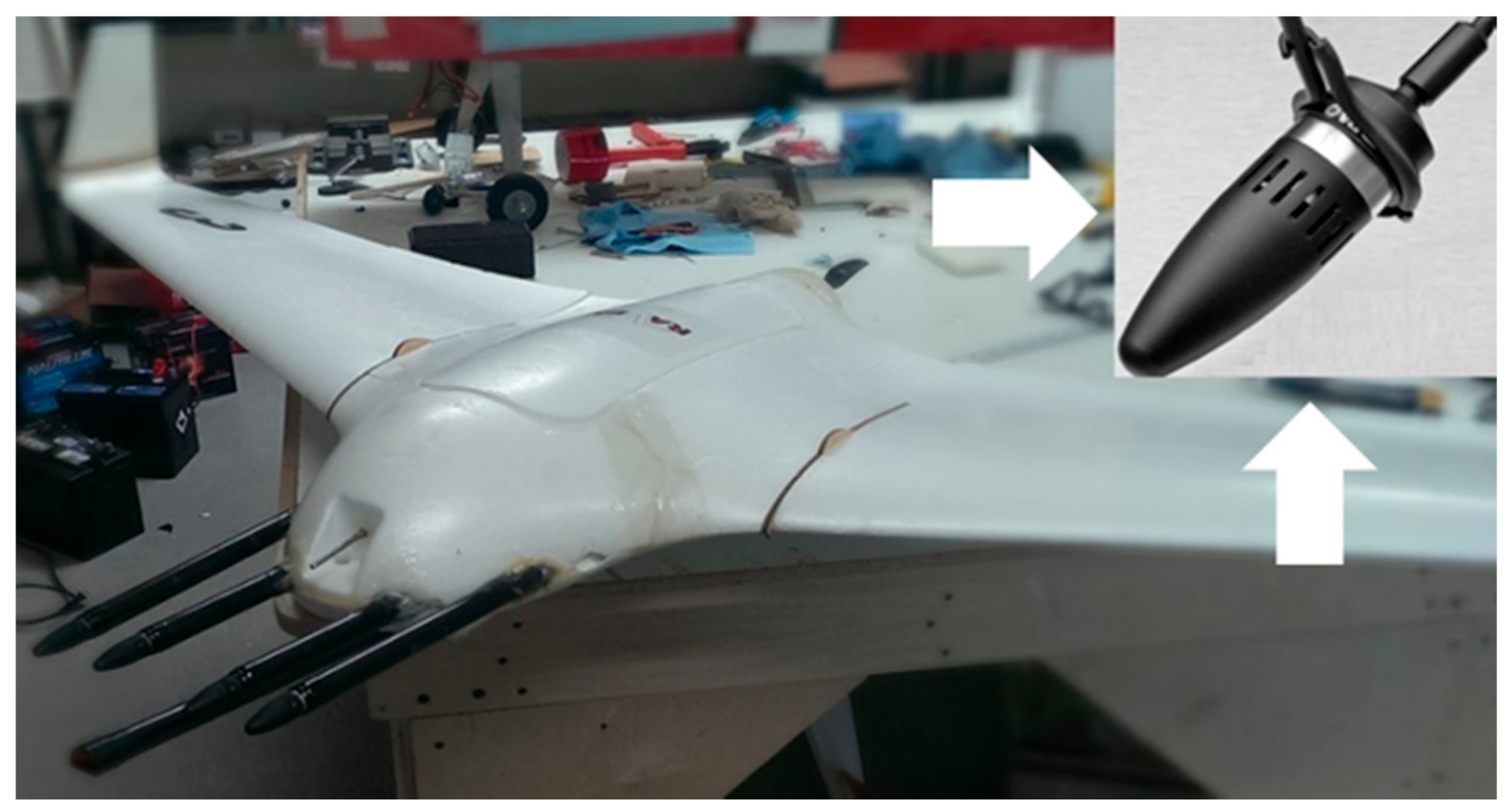
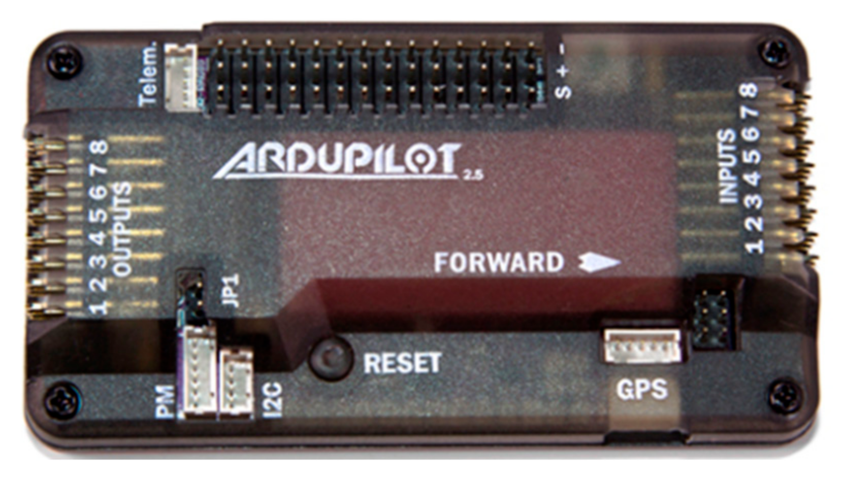
The sensing aircraft consisted of a hobby-grade Delta X-8 powered by a single brushless DC motor. Four DPA 4053 omnidirectional microphones were fitted to the aircraft via carbon fiber booms extending from the noise as depicted in Figure 3. The microphones were secured using custom vibration isolation mounts constructed from Sorbothane material. The intruding aircraft consisted of a gasoline-powered Giant Big Stik as displayed in Figure 4. Physical specifications for the two aircraft are also given in

Table 1. Aircraft specifications.

	Delta X-8	Giant Big Stik
Wingspan (m)	2.12	2.05
Length (m)	0.82	1.89
Mass (kg)	2.2	6.5
Payload Capacity (kg)	2–3	4–5
Cruising Speed (knots)	20–30	30–40
Sound Pressure Level (dBc @ 1 m)	NA	≈110–115

. Both aircraft were fitted with ArduPilot 2.5 systems for flight control and logging of data such as speed, Global Positioning System (GPS) position, altitude, and orientation. Figure 5 provides a picture of the device, while

Table 2. ArduPilot sensor accuracy values.

Data Type	Sensor Accuracy
GPS Position	±1.5 m
Compass Orientation (3D)	±2.5°
Altitude	±5 m
Airspeed	±1 m/s

lists the approximate sensor accuracy values. Acoustic data were recorded at a sampling rate of 48 KHz using a portable Zoom H4 handheld recording unit located inside the sensing aircraft.

3. Data Analysis

3.1. Signal Processing Overview

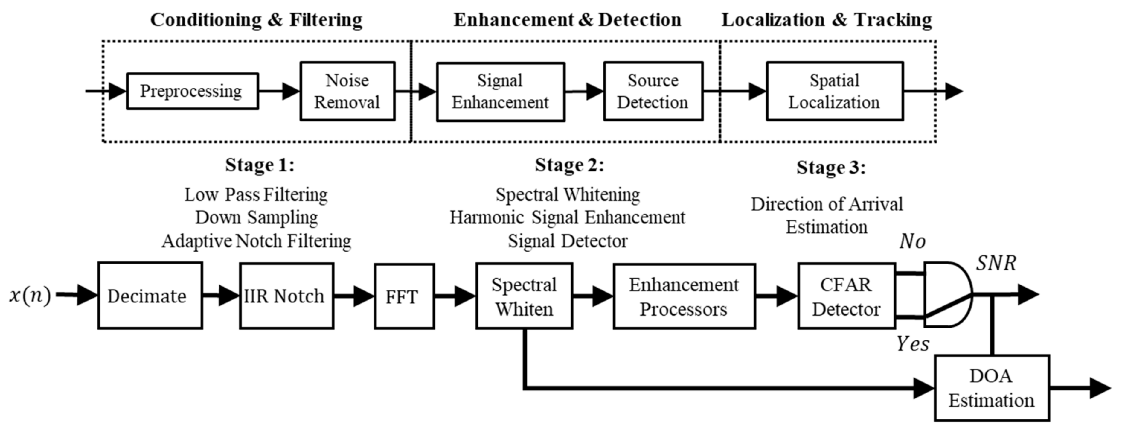
Once the acoustic signals had been digitally acquired, various processing steps were implemented to enable source detection and spatial localization. The required processing steps may be sectioned into three main stages with each stage containing multiple sub-operations as depicted in Figure 6. The major processing operations consist of: (1) conditioning and filtering; (2) enhancement and detection; and (3) localization and tacking. Recorded signals were first decimated to reduce data processing requirements since the recorded sampling was 48 kHz, but only information to up approximately 1000 Hz was found to be useful. The sample-reduced signals were then notch filtered to remove narrowband self-noise components using the referenceless adaptive Infinite Impulse Response (IIR) approach previously proposed by Tan [27,28,29,30]. The filtered signals were then windowed, frequency transformed using the Fast Fourier Transform (FFT) operation, and spectrally whitened via the Constant False Alarm Rate (CFAR)-enhanced method previously presented by Harvey and O’Young [31]. This procedure was performed to transform the broadband noise components to an equivalent distribution type to facilitate the use of the distribution-free CFAR (DF-CFAR) detector as proposed by Sarma and Tuffs [32]. Prior to performing detection operations, signals were first enhanced using the proposed Harmonic Spectral Transforms, which increase detection capabilities by exploiting the presence of multiple data channels in conjunction with the peak periodicity associated with harmonic signals in the frequency domain. Finally, if a target source signal is found to be present, the direction of arrival (DOA) may be estimated using an approach such as the steered response power (SRP) method. It should be noted, however, that details regarding localization and tracking of the intruding aircraft are not presented in the current paper due to the increased length it would entail; they will instead be presented in a future paper along with a beamforming method, which exploits the harmonic nature of signals to enhance DOA accuracy.

3.2. Harmonic Spectral Transforms

The presence of harmonic components is an inherent property of many acoustic signals such as those generated by voiced speech, musical instruments, and aircraft propulsion systems [33,34,35,36]. It arises from the presence of a physical boundary, which establishes the condition for standing wave generation [37]. One of the properties of such signals is that frequency spectra will exhibit periodic peaks located across its bandwidth. Processors have been successfully developed to exploit this property for increased pitch detection accuracy; perhaps, the most popular is the Harmogram proposed by Hinch [38] and the Harmonic Product Spectrum (HPS) proposed by Schroeder [39]. However, such processing methods may also be used for increased signal detection. Pitch detection differs from the general detection of harmonic signals in that the former assumes the presence of the signal to an appreciable degree and attempts to estimate its harmonic component structure, while the latter simply attempts to determine the presence of such a signal without much regard to structure.

Since the HPS and Harmogram are defined by taking either the sum or product of $R$ harmonically spaced components across the relevant frequency spectrum (magnitude for the HPS and power for the Harmogram), a more generalized function termed the Harmonic Spectral Transform (HST) can be defined according to the following:

$${\overline{\mathrm{H}}}_a[X(f)]={\left[\frac{1}{R}{\displaystyle \sum _{r=1}^R{\left|X(f\cdot r)\right|}^a}\right]}^{1/a}$$

(1)

where $X\left(f\right)$ is the relevant frequency spectrum and $a$ is an integer value that specifies the statistical mean form as given in

Table 3. Statistical mean forms of the harmonic spectral transform (HST).

Harmonic	Geometric	Standard	RMS
$a=-1$	$a=0$	$a=1$	$a=2$
${\left[\frac{1}{R}{\displaystyle \sum _{r=1}^R{\left|X(f\cdot r)\right|}^{-1}}\right]}^{-1}$	${\left[{\displaystyle \prod _{r=1}^R\left|X(f\cdot r)\right|}\right]}^{1/R}$	$\left[\frac{1}{R}{\displaystyle \sum _{r=1}^R\left|X(f\cdot r)\right|}\right]$	${\left[\frac{1}{R}{\displaystyle \sum _{r=1}^R{\left|X(f\cdot r)\right|}^2}\right]}^{1/2}$

.

Typically, the HST would be applied across some frequency band of interest where the fundamental component is believed to reside. The maximum possible range is given by $\left[0,f_s/2R\right]$ where $f_s$ is the sampling frequency. The fundamental frequency $f_o$ is then indicated by the location of the maximum spectral value according to:

$$f_o=\mathrm{ArgMax}\left[{\overline{\mathrm{H}}}_a[X(f)]\right].$$

(2)

If multiple channels are available for processing, the compounding operation may also be applied across channels to achieve further enhancement. For a system consisting of $S$ signals, the Multichannel Harmonic Spectral Transform (MHST) is, therefore, defined according to:

$${\overline{\mathrm{H}}}_{a,b}[X_s(f)]={\overline{\mathrm{H}}}_b\left[{\overline{\mathrm{H}}}_a[X_s(f)]\right]$$

(3)

where $X_s\left(f\right)$ is the frequency spectrum for the s^th signal. Expanding out the above form gives:

$${\overline{\mathrm{H}}}_{a,b}[X_s(f)]={\left[\frac{1}{S}{{\displaystyle \sum _{s=1}^S\left[{\left[\frac{1}{R}{{\displaystyle \sum _{r=1}^R\left|X_s(f\cdot r)\right|}}^a\right]}^{1/a}\right]}}^b\right]}^{1/b}$$

(4)

If multiple time realizations are available (FFT windows), further enhancement may be achieved by applying the operation across all channels and realizations. Thus, for a system consisting of $S$ signals with $W$ windowed time realizations, the Generalized Harmonic Spectral Transform (GHST) may be defined as:

$${\overline{\mathrm{H}}}_{a,b,c}[X_{s,w}(f)]={\overline{\mathrm{H}}}_c\left[{\overline{\mathrm{H}}}_b\left[{\overline{\mathrm{H}}}_a[X_{s,w}(f)]\right]\right]$$

(5)

Expanding out the above form thus gives:

$${\overline{\mathrm{H}}}_{a,b,c}[X_{s,w}(f)]={\left[\frac{1}{W}{{\displaystyle \sum _{w=1}^W\left[{\left[\frac{1}{S}{{\displaystyle \sum _{s=1}^S\left[{\left[\frac{1}{R}{{\displaystyle \sum _{r=1}^R\left|X_{s,w}(f\cdot r)\right|}}^a\right]}^{1/a}\right]}}^b\right]}^{1/b}\right]}}^c\right]}^{1/c}$$

(6)

To obtain a more informative symbolic expression, the GHST defined above may be expressed using the following notational form instead, which now indicates the total number of harmonics $R$, signals $S$, and windowed segments $W$ used:

$${\overline{\mathrm{H}}}_{a,b,c}\left[\right]\to {\overline{\mathrm{H}}}_{<a,b,c>}^{<R,S,W>}\left[\right]$$

(7)

It is apparent from the above equations that the proposed transforms closely resemble that of the ${\mathrm{AWSUM}}_k$ processors proposed by Wagstaff [40,41]. However, the transforms are in fact different since they are defined primarily for operations involving harmonic signals in which the peak periodicity of spectra is exploited. In contrast, the ${\mathrm{AWSUM}}_k$ processors do not exploit this spectral feature and are, instead, used primarily for single channel systems with a large number of time realizations. It should also be noted that the above transforms are not limited to standard magnitude or power spectra; it can be applied to any frequency-based spectrum that exhibits peak periodicity across the bandwidth of interest, such as that obtained via the coherence function [42].

3.3. Distribution-Free CFAR Detection

The DF-CFAR detector was previously proposed by Sarma and Tuffs as a means to detect unknown signals in noise of unknown statistical properties [32]. In line with the modified order statistic form presented by Harvey, it is given by the following [43]:

$$P_{fa}=\frac{\overline{k}+I}{N-G+1}$$

(8)

where $N$ is the number of noise samples contained in the noise bandwidth set defined by $\stackrel{\rightharpoonup }{N}$, $\overline{k}$ is the reversed order statistic number (the $\overline{k}$^th—largest value of $\stackrel{\rightharpoonup }{N}$), $G$ is the number of guard cells, and $I$ is the number of interfering targets.

Unlike other CFAR detectors such as the CA-CFAR and OS-CFAR, the DF-CFAR does not require noise to exhibit a specific distribution but instead requires only noise components to exhibit equivalent distribution forms. However, the performance of the detector is not completely impervious to the application of signal enhancement processors. Such a case would include use of the Harmonic Spectral Transforms (HSTs) previously presented. One of the issues with the transform process is that signal components are generated that are fractional values of the fundamental peak at various locations along the spectrum, where previously only noise would have resided. Failure to exclude these values from the noise sample set used to determine the test statistic will thus reduce detection performance to some degree, and/or produce inaccurate false alarm rates.

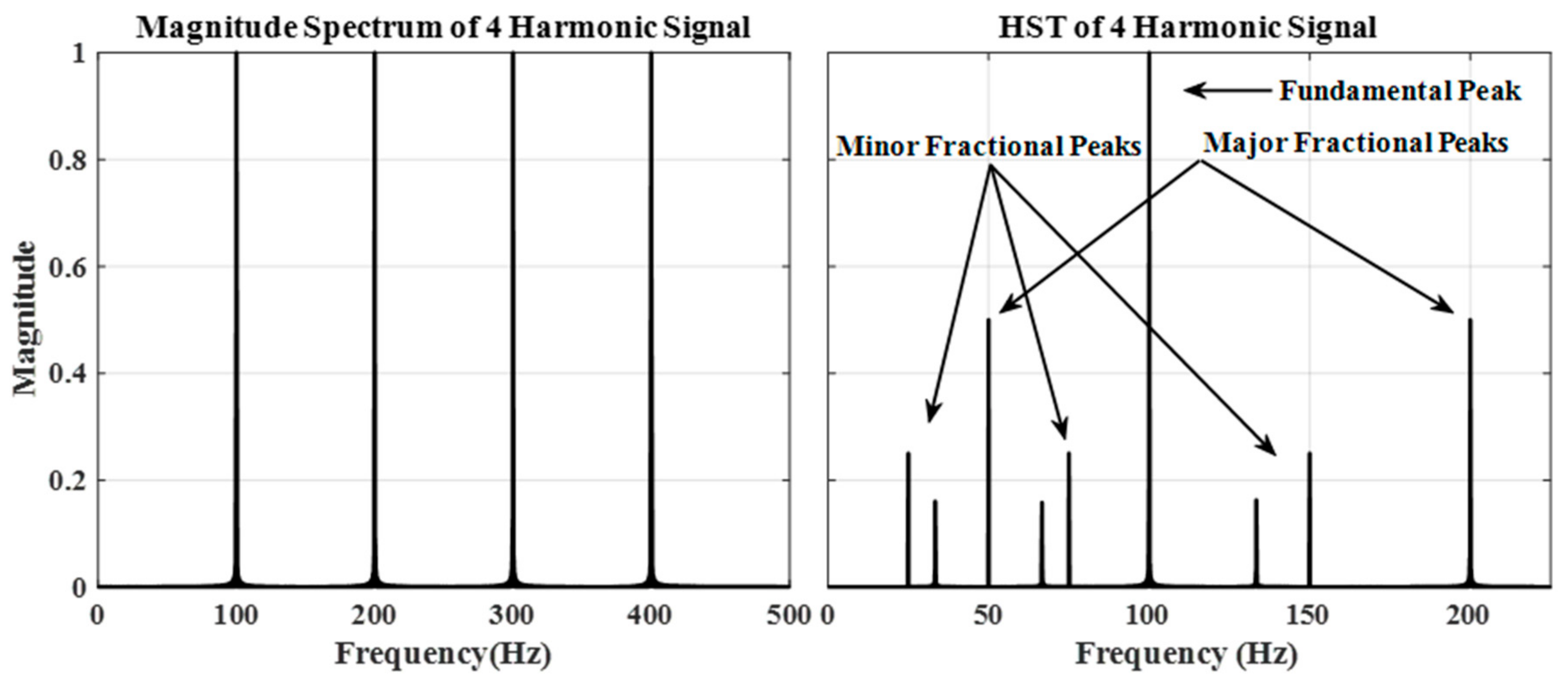
Figure 7 provides spectral plots of the FFT magnitude and standard mean HST $({\overline{\mathrm{H}}}_1)$ for a signal containing four harmonic components. From the plots, it is evident that the HST spectrum achieves a maximum at the fundamental frequency since all harmonic components are directly combined. It also contains smaller peaks located at frequencies that are fractions of one or more of those harmonic components. The location of all peaks (fractional and fundamental) will be contained in the set generated by:

$$f_{a,b}=\frac{a{f}_0}{b}$$

(9)

where $a,b\in \left\{1,2,\dots ,R\right\}$, $f_0$ is the fundamental frequency value and $R$ is the total number of harmonics. The number of fractional peaks will be given by the number of unique values (excluding the fundamental) contained in the set defined by $f_{a,b}$ up to the maximum value of $2f_0$.

Table 4. Number of fractional peaks present for HSTs of length $2f_o$.

Harmonics ($\mathit{R}$)	Fractional Peaks ($\mathit{F}$)
2	2
3	5
4	8
5	14
6	17
7	26
8	32

provides the number of fractional peaks for a given number of signal harmonics.

Since the DF-CFAR requires all noise components to exhibit equivalent distribution types in order to maintain a constant false alarm rate, fractional peak components must be excluded from the noise estimate. One may be tempted to treat the fractional components as simply target interference, in which case the false alarm probability would be given by Equation (8). However, doing so would also produce unnecessarily high false alarm rates. Because peak locations may be calculated for a given test cell frequency, they may instead be omitted from the noise estimate altogether. If $F$ number of fractional peaks are omitted, the false alarm rate will now be given by:

$$P_{fa}=\frac{\overline{k}+I}{N-F(G_F+1)-G+1}$$

(10)

where $G_F$ is the total number of guard cells placed about each fractional peak if desired. Note that the above equation only provides the false alarm rate for testing a single cell (SC) contained in the FFT spectrum. If evaluating $B$ test cells across a given spectrum, the total false alarm rate is given by the following [43]:

$$P_{FA}^{BI}={\displaystyle \sum }_{m=1}^B\left[{\left(-1\right)}^{(m+1)}\left(\begin{array}{c}B\\ m\end{array}\right){\displaystyle \prod }_{n=1}^m\left({\displaystyle \sum }_{r=D}^T\frac{{\left(1-{\stackrel{⌢}{P}}_n\right)}^{T-r}{{\stackrel{⌢}{P}}_n}^{r}T!}{\left(T-r\right)!r!}\right)\right]$$

(11)

where $D$ is the total number of detections required from $T$ trials (FFT windows) before confirming a detection. This procedure is known as binary integration (BI). For the case of $D=T$, the above form now gives the probability for a single trial (ST):

$$P_{FA}^{ST}={\displaystyle \sum }_{m=1}^B\left[{\left(-1\right)}^{(m+1)}\left(\begin{array}{c}B\\ m\end{array}\right){\displaystyle \prod }_{n=1}^B{\left({\stackrel{⌢}{P}}_n\right)}^T\right]$$

(12)

If the robust binary integration (RBI) method previously described by Harvey is applied, the total false alarm rate will now be given by [43]:

$$P_{FA}^{RBI}\approx {\displaystyle \sum }_{m=1}^B\left[{\left(-1\right)}^{(m+1)}\left(\begin{array}{c}B\\ m\end{array}\right){\displaystyle \prod }_{n=1}^B\left({\stackrel{⌢}{P}}_n{\left[1-{\left(1-{\stackrel{⌢}{P}}_n\right)}^{2\Delta +1}\right]}^{T-1}\right)\right]$$

(13)

$${\stackrel{⌢}{P}}_n=\frac{\overline{k}-n+I+1}{N-n-F(G_F+1)-G+2}$$

(14)

Note that Equations (11)–(14) constitute the constrained distribution-free CFAR (CDF-CFAR) detector [43].

3.4. Kinematic Considerations

In order to construct a viable acoustic-based SAA system, detection distances must be large enough to facilitate an avoidance maneuver. Currently, no official requirements exist but it is generally accepted that 500 ft (152.4 m) is the absolute minimum that should be maintained between aircraft at all times [1]. Direct analysis of the governing kinematic equations for two aircraft on a potential collision course leads to a series of expressions that cannot be solved directly using analytical methods. Geyer produced a solution for the direct head-on case by approximating the avoidance maneuver via a Taylor series expansion, producing the following equation [1]:

$$d_o\approx 5.6V_{rel}\sqrt{\frac{\pi }{2}-\varphi }$$

(15)

where $d_o$ is the minimum distance to initiate the avoidance maneuver to avoid a collision, $v_{rel}$ is the relative approaching speed of the two aircraft, and $\varphi$ is the bank (roll) angle initiated by the sensing aircraft upon detection. However, as admitted by Geyer, the approximation model is not appropriate for the small distances and velocities associated with UAV operations. For example, consider two aircraft with a closing velocity of $v_{rel}=50$ knots, where a bank angle of $\varphi =\pi /4$ rads is initiated by the sensing aircraft. Equation (15) gives a minimum detection distance of 127.6 m, which is less than the minimum accepted threshold of 152.4 m. Since the model proposed by Geyer is not appropriate for work pertaining to the present experiment, a simplistic analytical two-dimensional model is proposed that is more appropriate for UAV operations.

Consider the case for a detecting and an intruding aircraft both having constant speeds and headings of $\left|{\stackrel{\rightharpoonup }{v}}_{\alpha }\right|,\alpha$ and $\left|{\stackrel{\rightharpoonup }{v}}_{\beta }\right|,\beta$ respectively. Given the initial angular position $\gamma$ of the intruding aircraft with respect to the detecting aircraft (in the GPS coordinate system), we wish to find the minimum distance $\left|{\stackrel{\rightharpoonup }{d}}_o\right|$ that can facilitate an avoidance maneuver such that separation never falls below the collision boundary radius $r_b$. We assume that once the intruding aircraft is discovered, the detecting aircraft immediately initiates an instantaneous bank (roll) angle $\varphi$, and holds that angle until it reaches a new heading that is perpendicular to and away from the intruding aircraft’s flight path. Figure 8 provides a visual depiction of the system kinematic configuration. For sake of simplicity, the system is only defined in terms of two dimensions. Although the actual system is three dimensional, the 2-D model can provide a good approximation if the 3-D speed and heading values are projected on a 2-D plane connecting the two aircraft. In this regard, the 2-D model will produce a more conservative estimate, since one spatial degree of freedom is removed that may be used to perform the maneuver.

For a collision avoidance maneuver, there are three possible paths that can be taken:

• Head perpendicularly away from the intruder path by making the minimum bearing change.
• Head perpendicularly away from the intruder path by making the maximum bearing change.
• Adjust course to perpendicularly cross the intruder path.

Each of these cases are depicted in Figure 9. The choice between cases 1 and 2 may seem trivial at first but depending on the aircrafts’ headings, choosing the minimum bearing change may actually steer the sensing aircraft towards the intruder rather than away. However, when considering the actual kinematic and geometric configuration, this may still be the best course of action. The choice of which avoidance course to take for any given scenario requires a more complex analysis that is outside the scope of this paper. To simplify the analysis, we thus assume the aircraft adheres to avoidance case 1.

As previously stated, upon detection, the sensing aircraft initiates an instantaneous bank angle $\varphi$ that produces a turning radius $R_a$ (assuming constant altitude) given by:

$$R_a=\frac{v_{\alpha }^2}{\tan (\varphi )g}$$

(16)

Once the heading change is made, the sensing aircraft must then travel an additional distance $\left|{\stackrel{\rightharpoonup }{d}}_m\right|$ to avoid a collision:

$$d_m=r_b-\left|{\stackrel{\rightharpoonup }{r}}_{\varphi }\right|\sin \left(\psi \right)-\left|{\stackrel{\rightharpoonup }{r}}_{\alpha }\right|\left|{\widehat{r}}_{\alpha }•{\widehat{r}}_{\perp }\right|$$

(17)

The following relationships can be obtained via geometry as illustrated in Figure 8:

$$\theta ={\cos }^{-1}\left({\widehat{r}}_{\alpha }•{\widehat{r}}_{\perp }\right)$$

(18)

$$\psi =\left(\frac{\pi -\theta }{2}\right)$$

(19)

$$\left|{\stackrel{\rightharpoonup }{r}}_{\varphi }\right|=\sqrt{2R_a^2\left(1-\cos \left[\theta \right]\right)}$$

(20)

$$\left|{\stackrel{\rightharpoonup }{r}}_{\alpha }\right|=-\left|{\stackrel{\rightharpoonup }{d}}_o\right|\csc \left(\alpha -\beta \right)\sin \left(\beta -\gamma \right)$$

(21)

where ${\widehat{r}}_{\perp }$ is the direction perpendicular to ${\widehat{r}}_{\beta }$ that minimizes $\theta$ as given by the following expression:

$${\widehat{r}}_{\perp }=\langle -{\widehat{r}}_{\beta ,y},{\widehat{r}}_{\beta ,x}\rangle \vee \langle {\widehat{r}}_{\beta ,y},-{\widehat{r}}_{\beta ,x}\rangle .$$

(22)

The total time required to execute the heading change and travel the remaining distance $\left|{\stackrel{\rightharpoonup }{d}}_m\right|$ to reach a final perpendicular distance $r_b$ away from the intruder path is given by:

$$t_{avoid}=\frac{R\theta +\left|{\stackrel{\rightharpoonup }{d}}_m\right|}{\left|{\stackrel{\rightharpoonup }{v}}_{\alpha }\right|}$$

(23)

During this time, the intruder will advance a distance $\left|{\stackrel{\rightharpoonup }{r}}_{\beta }\right|$ given by:

$$\left|{\stackrel{\rightharpoonup }{r}}_{\beta }\right|=\left|{\stackrel{\rightharpoonup }{v}}_{\beta }\right|t_{avoid}$$

(24)

Thus, the initial radial separation distance required is given by:

$$\left|{\stackrel{\rightharpoonup }{d}}_o\right|=\frac{\left|{\stackrel{\rightharpoonup }{r}}_{\beta }\right|-{\widehat{r}}_{\alpha }•{\widehat{r}}_{\beta }\left|{\stackrel{\rightharpoonup }{r}}_{\varphi }\right|\cos \left(\psi \right)}{\left|{\widehat{d}}_o•{\widehat{r}}_{\beta }\right|}$$

(25)

Combining the above equations and solving for $\left|{\stackrel{\rightharpoonup }{d}}_o\right|$ gives the following final form:

$$\left|{\stackrel{\rightharpoonup }{d}}_o\right|=\frac{\left|{\stackrel{\rightharpoonup }{v}}_{\beta }\right|\left(r_b+R_a\theta -\left|{\stackrel{\rightharpoonup }{r}}_{\varphi }\right|\cos \left[\theta /2\right]\right)+\left|{\stackrel{\rightharpoonup }{r}}_{\varphi }\right|\left|{\stackrel{\rightharpoonup }{v}}_{\alpha }\right|\left[{\widehat{r}}_{\alpha }•{\widehat{r}}_{\beta }\right]\sin \left[\theta /2\right]}{\left|{\stackrel{\rightharpoonup }{v}}_{\alpha }\right|\left|{\widehat{d}}_o•{\widehat{r}}_{\beta }\right|-\left|{\stackrel{\rightharpoonup }{v}}_{\beta }\right|\left|{\widehat{r}}_{\alpha }•{\widehat{r}}_{\perp }\right|\csc \left[\alpha -\beta \right]\sin \left[\beta -\gamma \right]}$$

(26)

For the case of a head on collision course, the above equation reduces to:

$$\left|{\stackrel{\rightharpoonup }{d}}_o\right|=\frac{r_b\left|{\stackrel{\rightharpoonup }{v}}_{\beta }\right|}{\left|{\stackrel{\rightharpoonup }{v}}_{\alpha }\right|}+\frac{\left|{\stackrel{\rightharpoonup }{v}}_{\alpha }\right|\left(2\left|{\stackrel{\rightharpoonup }{v}}_{\alpha }\right|+\left|{\stackrel{\rightharpoonup }{v}}_{\beta }\right|\left[\pi -2\right]\right)\cot \left[\varphi \right]}{2g}$$

(27)

Utilizing Equation (26) in conjunction with typical cruising speeds for various aircraft, a list of approximate detection distances required for various heading scenarios has been constructed and is displayed in

Table 5. Minimum required detection distances for various aircraft.

Intruder Aircraft	Intruder Speed (knots)	${\mathit{d}}_{\mathit{o}}$ (m) ($\mathit{\beta }\mathbf{=}\mathbf{180}$, $\mathit{\gamma }\mathbf{=}\mathbf{0}$)
		$\mathit{\alpha }\mathbf{=}\mathbf{0}$	$\mathit{\alpha }\mathbf{=}\mathbf{45}$	$\mathit{\alpha }\mathbf{=}\mathbf{90}$
Giant Big Stik (UAV)	35	218	185	178
Cessna 185	95	551	494	483
Bell 206	115	662	600	584
Sikorsky S-92	140	795	725	711
Boeing 737	250 *	1402	1290	1270

* Maximum suggested airspeed from takeoff to 10,000 ft.

. For each case it is assumed that the initial angular position between the two aircraft is zero ($\gamma =0$), the avoiding aircraft initiates an instantaneous bank angle of $\varphi =\pi /4$ while travelling at 30 knots, and the collision boundary distance is $r_b=152.4$ m.

4. Results & Discussion

The experiment was originally conducted using a total of four microphones. However, a malfunctioning external power supply corrupted two of the channels with excess noise rendering them useless. Thus, data processing was performed using only two of the recorded signals. Since both aircraft were in relatively close proximity throughout the experiment, observed source frequencies were highly non-stationary. Because of this, the use of alternative methods such as coherence-based detection would not perform well since it requires a relatively stationary signal for an upwards of 4 to 6 windowed segments [42]. Instead, the signals were enhanced using the HSTs previously presented. The effectiveness of the technique is verified by comparing the results to that obtained via the standard incoherent mean as defined by the following:

$$\overline{X}(f)=\frac{1}{S}{\displaystyle \sum _{s=1}^S\left|X_s(f)\right|}$$

(28)

Table 6. Signal preprocessing and filter parameters.

Sampling Frequency ($f_s$)	48 kHz	Number of Signals	2
Decimation Factor	10	FFT Window	0.5 s
IIR Step Size ($\mu$)	5 × 10−4	Window Overlap	50%
Notch Radius ($r$)	0.995	Padded Length ($L_{fft}$)	6000 pts
Harmonics Removed ($H$)	8	Spectral Resolution ($f_r$)	0.5 Hz/bin

,

Table 7. CFAR-enhanced spectral whitening parameters.

Detector Type	OS-CFAR	Noise Samples (N)	101
Forgetting Factor ($\xi$)	0.2	Order Statistic ($k$)	$0.75\times N$
Flooring Factor ($\delta$)	0.5	Guard Cell Band ($\stackrel{\rightharpoonup }{G}$)	5.5 Hz
Noise Band ($\stackrel{\rightharpoonup }{N}$)	50 Hz	Guard Cells ($G$)	12

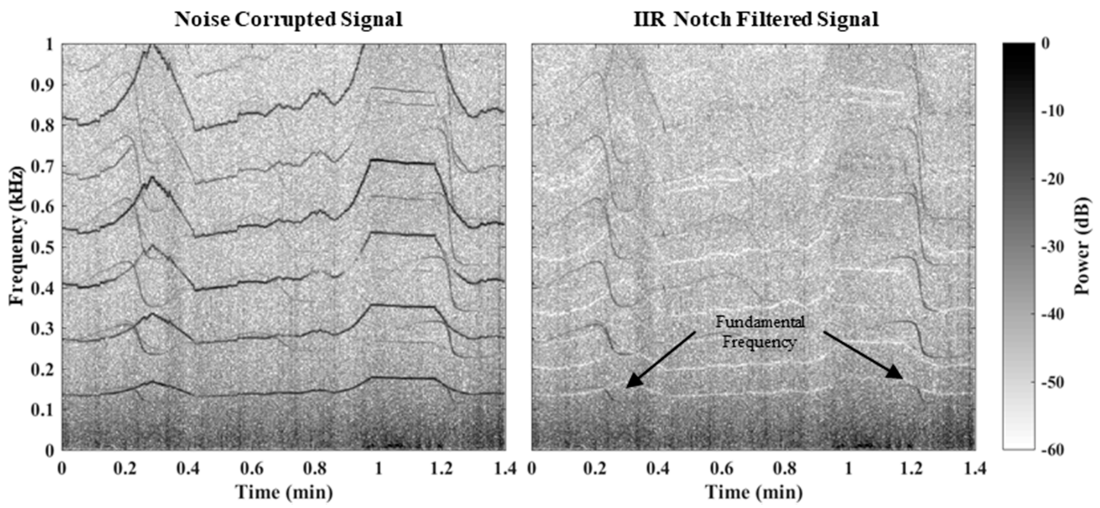
and

Table 8. SCDF-CFAR detection parameters.

	${\overline{\mathbf{H}}}_{\mathbf{1}}\mathbf{\left[}\mathit{X}\mathbf{\right]}$	$\overline{\mathit{X}}$		${\overline{\mathbf{H}}}_{\mathbf{1}}\mathbf{\left[}\mathit{X}\mathbf{\right]}$	$\overline{\mathit{X}}$
Noise Sample Band ($\stackrel{\rightharpoonup }{N}$)	10–400 Hz	10–492.5 Hz	Order Statistic ($\overline{k}$)	3	3
Test Band ($\stackrel{\rightharpoonup }{B}$)	100–200 Hz	200–400 Hz	Consec. Trials ($T$)	3	3
Guard Cell Band ($\stackrel{\rightharpoonup }{G}$)	10 Hz	10 Hz	Consec. Detections ($D$)	3	3
Fract. Guard Band (${\stackrel{\rightharpoonup }{G}}_F$)	1 Hz	1 Hz	Cell Deviation ($\Delta$)	1	1
Noise Samples ($N$)	780 pts	965 pts	Maxima Tested ($M$)	3	3
Test Cells ($B$)	201 pts	401 pts	$P_{FA}^{SC}$	4.2 × 10−3	3.4 × 10−3
Guard Cells ($G$)	22 pts	22 pts	$P_{FA}^{ST}$	0.63	0.83
Fract. Guard Cells ($G_F$)	2 pts	2 pts	$P_{FA}^{BI}$	1.5 × 10−5	1.5 × 10−5
Fractional Peaks ($F$)	17	17	$P_{FA}^{RBI}$	1.4 × 10−4	1.4 × 10−4

provide the notch filter, FFT, spectral whitening, and SCDF-CFAR parameters used. Nonstationary narrowband noise generated by the sensing aircraft propulsion system was removed via the referenceless adaptive IIR notch filtering approach proposed by Tan [27,28,29,30], since the aircraft engine was running continuously throughout the experiment. Figure 10 provides sample spectrogram plots, which demonstrate the effectiveness of the adaptive IIR notch filtering approach.

Note that the selective cell distribution-free CFAR detector (SCDF-CFAR) previously presented by Harvey and O’Young was used [43]. In brief, it is essentially equivalent to the CDF-CFAR detector presented above by Equations (11)–(14), except only the $M$ largest cells contained in the test band $\stackrel{\rightharpoonup }{B}$ are evaluated instead of all $B$ cells. A more detailed explanation of this detector may be found in [43]. Two sets of detection parameters are provided in the table since two enhancement processors were used, which evidently have different spectral properties with regard to possible detector configurations. These included the standard incoherent mean ($\overline{X}$) and the standard mean HST (${\overline{\mathrm{H}}}_{\langle 11\rangle }^{\langle 6,2\rangle }\left[X\right]$) using six ($R=6$) harmonics. Since the recorded signals were decimated to a final sampling rate of 4800 Hz, the maximum noise frequency band only ranged from 0 to 400 Hz for the HST processor. In contrast, the incoherent mean was free to utilize noise samples across the entire signal bandwidth (0 to 2400 Hz). However, noise sample sizes were chosen such that each processor produced an equivalent false alarm rate as indicated in the table. In addition to the noise sample size, frequency test bands were also different for the two processed signal forms. The HST test band contained only the expected source fundamental frequency range (100 to 200 Hz). However, a visual analysis of the recorded signal spectra for the incoherent mean revealed that the second harmonic component was of much greater amplitude and thus better suited for detection. This effectively doubled the expected source frequency range (200 to 400 Hz) for that processor.

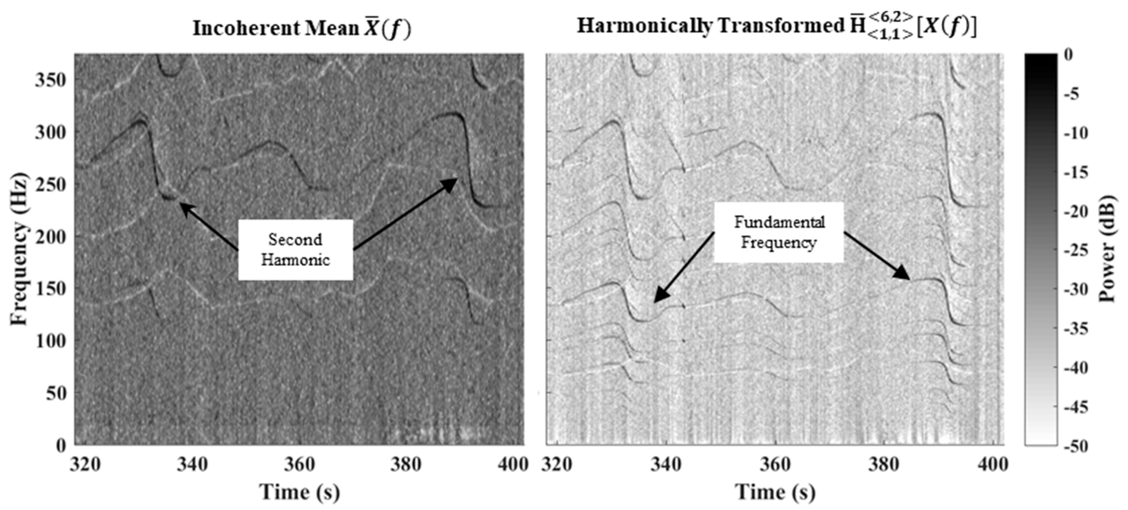
Presented false alarm probabilities for the HST were calculated using Equations (10)–(14). These equations were also used for the incoherent mean to maintain consistency, and because the fractional peak properties of the detection method would automatically exclude surrounding harmonic components from being included in the noise sample estimate. Figure 11 provides sample spectrogram plots of the average power and harmonically transformed signals. It is evident from the HST spectrogram that a large number of fractional peaks are in fact present. In theory, a total of 17 fractional peaks may be present as previously indicated by Table 4. In addition, it is clear the second harmonic component has the highest peak prominence for the incoherent mean form. This is also visible from the sample detection spectra displayed in Figure 12.

Table 9. Detection results.

	Detections (#)		Max Distance (m)		Mean Distance (m)
	$\overline{X}$	${\overline{\mathrm{H}}}_{\langle 11\rangle }^{\langle 6,2\rangle }\left[X\right]$	$\overline{X}$	${\overline{\mathrm{H}}}_{\langle 11\rangle }^{\langle 6,2\rangle }\left[X\right]$	$\overline{X}$	${\overline{\mathrm{H}}}_{\langle 11\rangle }^{\langle 6,2\rangle }\left[X\right]$
Single Trial (ST)	1077	1930	672	678	270	302
Binary Integration (BI)	215	551	498	572	205	240
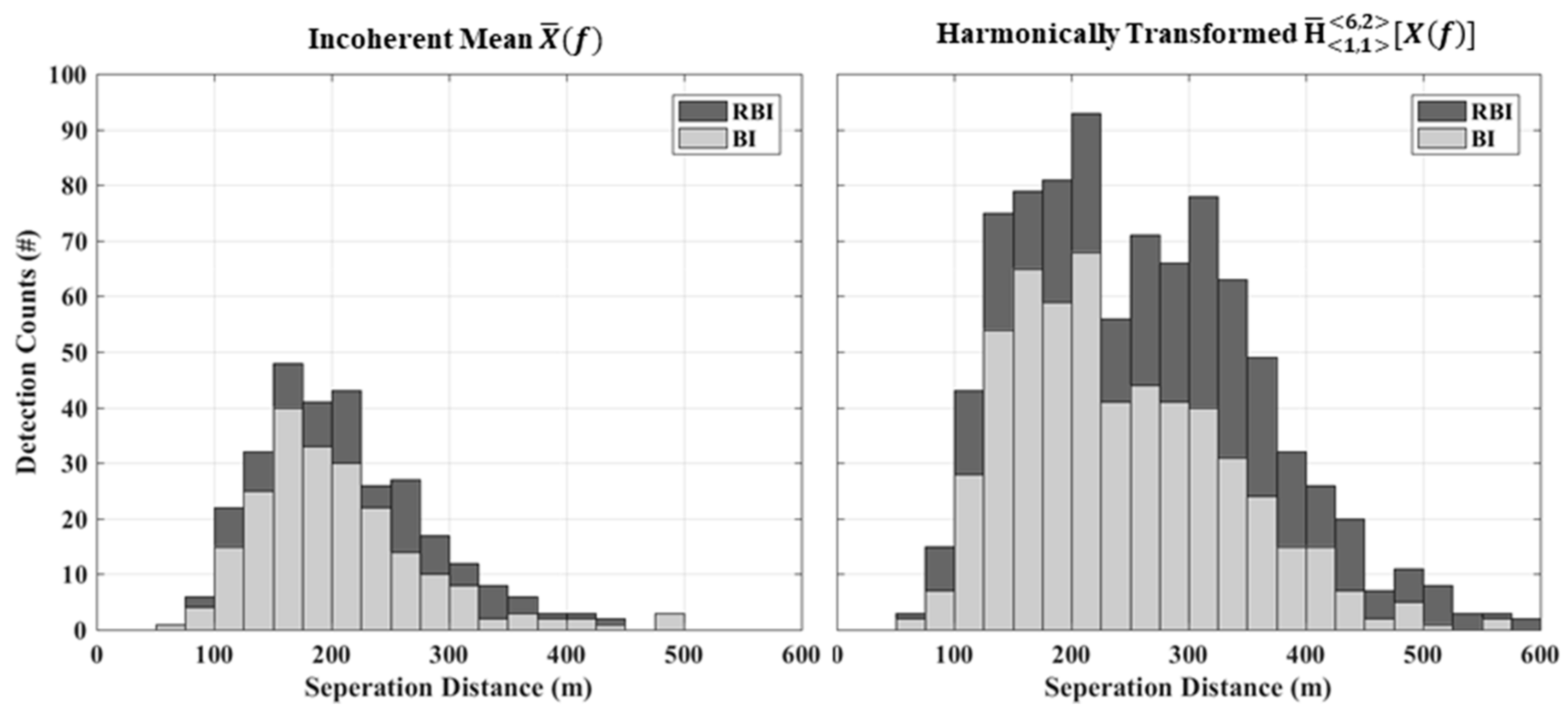
Robust Binary Integration (RBI)	300	884	500	593	212	258

provides the detection results for each enhancement processor and detection scheme. From a comparison of the results obtained, it is evident that the harmonically transformed signals produced the highest detectability for all three schemes. The total number of detections were nearly double for all cases, while detection distances were also significantly increased. A total of 1930 detections were achieved for the harmonically transformed signal, with a maximum and mean range of 678 and 302 m, respectively. It is apparent that the single trial (ST) method produced the highest number of detections. However, when considering the false alarm rate associated with this method ($P_{FA}^{ST}$) as given in Table 8, it is evident that values are too high for this detector to be of practical use. Binary integration (BI) was found to greatly reduce this value to an acceptable level, but at the expense of signal detectability. Since source signals were highly non-stationary as previously discussed, application of the robust binary integration (RBI) provided some alleviation to this issue. This is also evident in a more visual form via the histogram plots displayed in Figure 13. From the plots, it is visible that the RBI scheme provides a significant detectability increase in the 200 to 350 m range. This result is significant since this region dedicates the lower limit at which another UAV can be detected with adequate distance to perform an avoidance maneuver as previously indicated by Table 5.

Using the basic attenuation laws for acoustic propagation in an ideal medium, a crude approximation may also be obtained for the maximum detection distances achievable for other aircraft such as a Cessna, for example. Using the process previously outlined by Harvey and O’Young in [26], the following equation may be established:

$$d_{max}=d_{ref}{10}^{\frac{\Delta SPL}{20}}$$

(29)

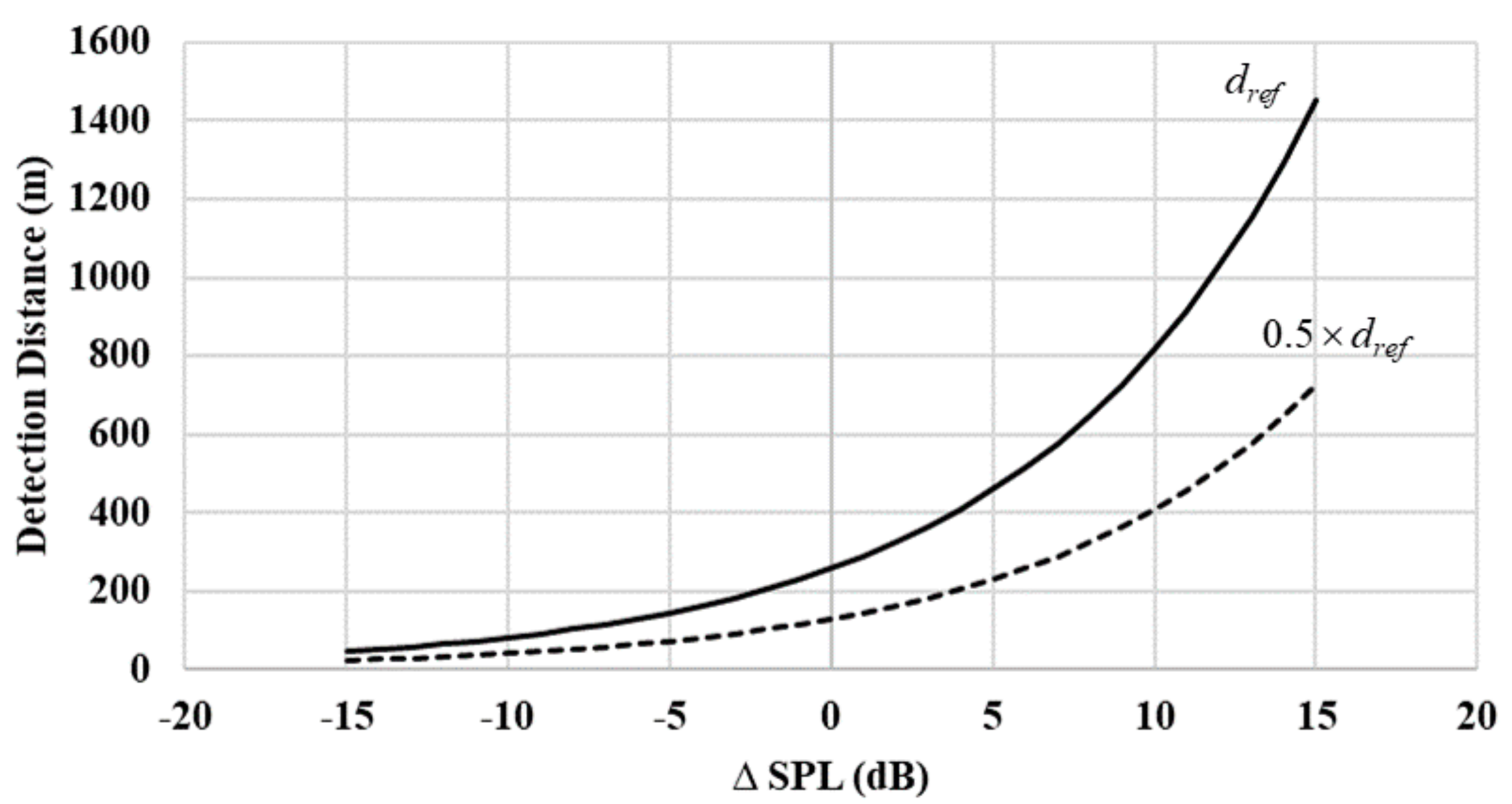
where $\Delta SPL$ is the effective Sound Pressure Level (in dB) difference between the current reference aircraft and some other source of concern, $d_{ref}$ is the reference distance at a point of detection, and $d_{max}$ is the maximum estimated detection distance for the target source. Since it was previously determined in [26] that a change in acoustic SPL (in dB) is directly proportional to a change in signal power (in dB), the above equation can be used to compare theoretical detection distances by simply replacing the change in SNR described in [26] by the difference in SPL level for the two acoustic sources. Figure 14 provides the maximum expected detection distances for a range of $\Delta SPL$ values using the Giant Big Stik UAV as the base reference level. Since atmospheric attenuation factors were omitted from the function form presented above by Equation (29), conservative estimates using 50% of the calculated values are also provided. A reference distance of 258 m was used, which is the mean detection distanced obtained via the HST method in conjunction with the RBI detection scheme as indicated in Table 9.

Consider, for example, a Cessna 185 that has an SPL of approximately 130 dB providing a $\Delta SPL$ level of 15 dB compared to the Giant Big Stik UAV [44]. According to Figure 14, the aircraft should be detectable somewhere between approximately 800 and 1400 m away. When examining the minimum detection distances required to avoid a collision as previously presented in Table 5, it appears the aircraft should have been detected with sufficient distance. Such results are also found to agree with that previously presented in [26]. Conversely, aircraft with a lower operating SPL, such as smaller UAVs, would be detected at shorter distances as indicated by the plot. Ultimately, experiments are required for a range of aircraft types to determine maximum detection distances, since the presented values assume ideal propagation conditions, which ignore effects such as wind, temperature gradients, ground conditions, etc.; all of these may reduce the actual detection distances.

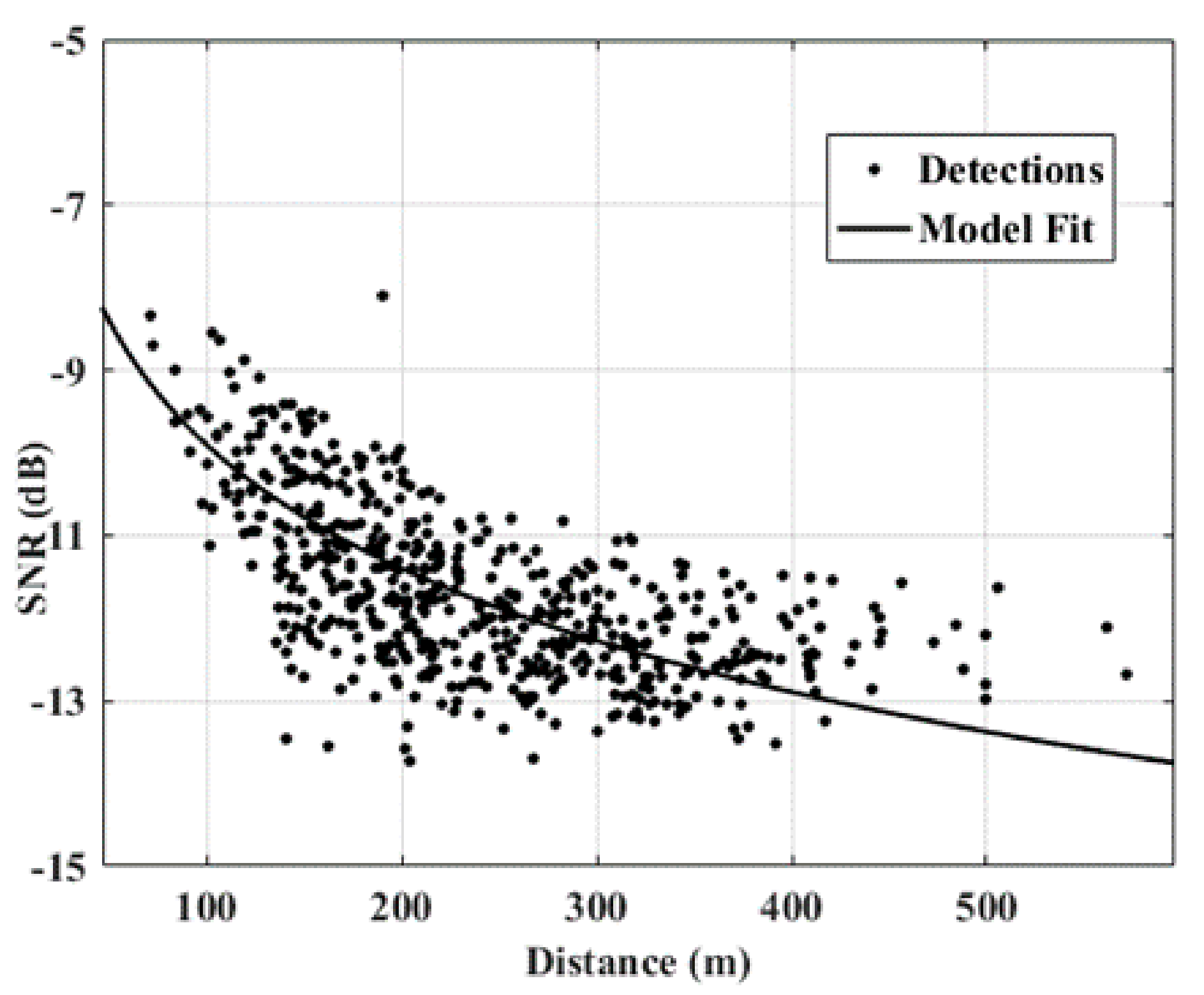
Figure 15 provides a plot of the SNR with respect to distance for each detection point. Since it was previously established in [26] that $SNR\propto SPL$, the observed values may be modeled using the acoustic attenuation laws according to:

$$SNR=-A\cdot 20{\log }_{10}\left(x\right)-B\cdot x$$

(30)

where $A$ represents the linear SPL/SNR proportionality or scaling constant and $B$ represents an atmospheric absorption factor. From the plot it is evident that the observed SNR values do follow the trend predicted by the model. This provides verification that the above extrapolation approach is valid.

5. Conclusions

The proposed harmonic spectra transform was found to provide a significant increase in the number of detections and maximum detection range compared to the standard incoherent mean. Detection distances up to 678 m were achieved, which is more than double the minimum required to avoid a head-on collision according to the presented model. Although the single trial testing scheme produced false alarm rates that are too high to constitute a practical detector, the application of the binary integration approach provided a substantial reduction in values while modestly affecting detection distances. The robust binary integration scheme provided a significant increase in detectability compared to the binary integration method since source signals were highly non-stationary. However, this increase was attained at the cost of increasing the false alarm rate by a full order of magnitude. Based on the overall results obtained, it can be concluded that the Giant Big Stik UAV was detected with sufficient distance to perform an avoidance maneuver. Thus, acoustic sensing may, in fact, be a viable technology to establish a non-cooperative collision avoidance system. However, results regarding the ability of the system to localize and track detected targets are still required before any definitive conclusions can be made.

References

- Geyer, C.; Singh, S.; Chamberlain, L. Avoiding Collisions between Aircraft: State of the Art and Requirements for UAVs Operating in Civilian Airspace; Technique Reports; CMU-RI-TR-08-03; Robotics Institute, Carnegie Mellon University: Pittsburgh, PA, USA, 2008. [Google Scholar]
- Finn, A.; Franklin, S. Acoustic sense & avoid for UAV’s. In Proceedings of the 7th International Conference on Intelligent Sensors, Sensor Networks and Information Processing (ISSNIP), Adelaide, Australia, 6–9 December 2011. [Google Scholar]
- Zelnio, A.M.; Case, E.E.; Rigling, B.D. A low-cost acoustic array for detecting and tracking small RC aircraft. In Proceedings of the 2009 IEEE 13th Digital Signal Processing Workshop and 5th IEEE Signal Processing Education Workshop, Marco Island, FL, USA, 4–7 January 2009. [Google Scholar]
- Case, E.E.; Zelnio, A.M.; Rigling, B.D. Low-cost acoustic array for small UAV detection and tracking. In Proceedings of the 2008 IEEE National Aerospace and Electronics Conference, Dayton, OH, USA, 16–18 July 2008. [Google Scholar]
- Zelnio, A.M. Detection of Small Aircraft Using an Acoustic Array; Wright State University: Fairborn, OH, USA, 2009. [Google Scholar]
- Sutin, A.; Salloum, H.; Sedunov, A.; Sedunov, N. Acoustic detection, tracking and classification of low flying aircraft. In Proceedings of the 2013 IEEE International Conference on Technologies for Homeland Security (HST), Waltham, MA, USA, 12–14 November 2013. [Google Scholar]
- Salloum, H.; Sedunov, A.; Sedunov, N.; Sutin, A.; Masters, D. Acoustic system for low flying aircraft detection. In Proceedings of the 2015 IEEE International Symposium on Technologies for Homeland Security (HST), Waltham, MA, USA, 14–16 April 2015. [Google Scholar]
- Nielsen, R.O. Acoustic detection of low flying aircraft. In Proceedings of the IEEE Conference on Technologies for Homeland Security, Boston, MA, USA, 11–12 May 2009. [Google Scholar]
- Ferguson, B.G. A ground-based narrow-band passive acoustic technique for estimating the altitude and speed of a propeller-driven aircraft. J. Acoust. Soc. Am. 1992, 92, 1403–1407. [Google Scholar] [CrossRef]
- Sadasivan, S.; Gurubasavaraj, M.; Sekar, S. Acoustic signature of an unmanned air vehicle exploitation for aircraft localisation and parameter estimation. Def. Sci. J. 2002, 51, 279. [Google Scholar] [CrossRef]
- Tong, J.; Xie, W.; Hu, Y.; Bao, M.; Li, X.; He, W. Estimation of low-altitude moving target trajectory using single acoustic array. J. Acoust. Soc. Am. 2016, 139, 1848–1858. [Google Scholar] [CrossRef] [PubMed]
- Ferguson, B.G.; Lo, K.W. Turbo-prop and rotary-wing aircraft flight parameter estimation using both narrow-band and broadband passive acoustic signal processing methods. J. Acoust. Soc. Am. 2000, 108, 1763–1771. [Google Scholar] [CrossRef] [PubMed]
- Reiff, C.; Pham, T.; Scanlon, M.; Noble, J.; Landuyt, A.V.; Petek, J.; Ratches, J. Acoustic Detection from an Aerial Balloon Platform; US Army Research Laboratory: Adelphi, MD, USA, 2004. [Google Scholar]
- Lo, K.W.; Ferguson, B.G. Tactical unmanned aerial vehicle localization using ground-based acoustic sensors. In Proceedings of the 2004 Intelligent Sensors, Sensor Networks, and Information Processing Conference, Melbourne, Australia, 14–17 December 2004. [Google Scholar]
- Tong, J.; Hu, Y.-H.; Bao, M.; Xie, W. Target tracking using acoustic signatures of light-weight aircraft propeller noise. In Proceedings of the IEEE China Summit & International Conference on Signal and Information Processing (ChinaSIP), Beijing, China, 6–10 July 2013. [Google Scholar]
- Pham, T.; Srour, N. TTCP AG-6: Acoustic detection and tracking of UAVs. In Proceedings of the International Society for Optical Engineering, Orlando, FL, USA, 1 September 2004. [Google Scholar]
- Silva, R.A. Numerical Simulation and Laboratory Testing of Time-Frequency MUSIC Beamforming for Identifying Continuous and Impulsive Ground Targets from a Mobile Aerial Platform; Texas A&M University: College Station, TX, USA, 2013. [Google Scholar]
- Tijs, E.; Yntema, D.; Wind, J.; de Bree, H.E. Acoustic Vector Sensors for Aeroacoustics. CEAS Buchares. 2009. Available online: http://www.microflown.com/files/media/library/Publications/Farfield/2009_ceas.pdf (accessed on 6 November 2017).
- Tijs, E.H.G.; de Croon, G.C.H.E.; Wind, J.W.; Remes, B.; de Wagter, C.; de Bree, H.E.; Ruijsink, R. Hear-and-avoid for micro air vehicles. In Proceedings of the International Micro Air Vehicle Conference and Competitions (IMAV), Braunschweig, Germany, 6–8 July 2010. [Google Scholar]
- Ferguson, B.; Wyber, R. Detection and localization of a ground based impulsive sound source using acoustic sensors onboard a tactical unmanned aerial vehicle. In Proceedings of the Symposium on Battlefield Acoustic Sensing for ISR Applications, Amsterdam, The Netherlands, 9–10 October 2006. [Google Scholar]
- Robertson, D.N.; Pham, T.; Edge, H.; Porter, B.; Shumaker, J.; Cline, D. Acoustic sensing from small-size UAVs. In Proceedings of the SPIE Defense and Security Symposium, Orlando, FL, USA, 9–13 April 2007. [Google Scholar]
- Ohata, T.; Nakamura, K.; Mizumoto, T.; Taiki, T.; Nakadai, K. Improvement in outdoor sound source detection using a quadrotor-embedded microphone array. In Proceedings of the IEEE/RSJ International Conference on Intelligent Robots and Systems (IROS), Chicago, IL, USA, 14–18 September 2014. [Google Scholar]
- Okutani, K.; Yoshida, T.; Nakamura, K.; Nakadai, K. Outdoor auditory scene analysis using a moving microphone array embedded in a quadrocopter. In Proceedings of the IEEE/RSJ International Conference on Intelligent Robots and Systems (IROS), Vilamoura, Portugal, 7–12 October 2012; p. 3288. [Google Scholar]
- Scientific Applications and Research Associates Inc. (SARA). UAV Acoustic Collision-Alert System. 2012. Available online: http://www.sara.com/ISR/UAV_payloads/PANCAS.html (accessed on 4 September 2017).
- Milkie, T. Passive Acoustic Non-Cooperative Collision Alert System (PANCAS) for UAV Sense and Avoid; SARA, Inc.: Cypress, CA, USA, 2007; unpublished white paper. [Google Scholar]
- Harvey, B.; O’Young, S. Detection of continuous ground-based acoustic sources via unmanned aerial vehicles. J. Unmanned Veh. Syst. 2015, 4, 83. [Google Scholar] [CrossRef]
- Tan, L.; Jiang, J. Novel adaptive IIR filter for frequency estimation and tracking [DSP Tips & Tricks]. IEEE Signal Process. Mag. 2009, 26, 186–189. [Google Scholar]
- Tan, L.; Jiang, J. Real-Time Frequency Tracking Using Novel Adaptive Harmonic IIR Notch Filter. Technol. Interface J. 2009, 9. [Google Scholar] [CrossRef]
- Tan, L.; Jiang, J. Simplified Gradient Adaptive Harmonic IIR Notch Filter for Frequency Estimation and Tracking. Am. J. Signal Process. 2015, 5, 6–12. [Google Scholar]
- Tan, L.; Jiang, J.; Wang, L. Adaptive harmonic IIR notch filters for frequency estimation and tracking. In Adaptive Filtering; Garcia, L., Ed.; InTech: London, UK, 2011; p. 313. [Google Scholar]
- Harvey, B.; O’Young, S. A CFAR-Enhanced Spectral Whitening Method for Acoustic Sensing via UAVs. Drones 2018, 2, 1. [Google Scholar] [CrossRef]
- Sarma, A.; Tufts, D.W. Robust adaptive threshold for control of false alarms. IEEE Signal Process. Lett. 2001, 8, 261–263. [Google Scholar] [CrossRef]
- Marte, J.E.; Kurtz, D.W. A Review of Aerodynamic Noise from Propellers, Rotors, and Lift Fans; Technique Reports 32-1462; NASA Jet Propulsion Laboratory: Pasadena, CA, USA, 1970. [Google Scholar]
- Stevens, K.N. Acoustic Properties used for the Identification of Speech Sounds. Ann. N. Y. Acad. Sci. 1983, 405, 2–17. [Google Scholar] [CrossRef] [PubMed]
- McAdams, S.; Depalle, P.; Clarke, E. Analyzing musical sound. In Empirical Musicology: Aims, Methods, Prospects; Clarke, E., Ed.; Oxford University Press: New York, NY, USA, 2004; pp. 157–196. [Google Scholar]
- Farassat, F.; Brentner, K.B. The Acoustic Analogy and the Prediction of the Noise of Rotating Blades. Theor. Comput. Fluid Dyn. 1998, 10, 155–170. [Google Scholar] [CrossRef]
- TerMeulen, R.B. Notes on Acoustics for Undergraduates. M. Eng.; Pennsylvania State University: Pennsylvania, PA, USA, 2008. [Google Scholar]
- Hinich, M. Detecting a hidden periodic signal when its period is unknown. IEEE Trans. Acoust. Speech Signal Process. 1982, 30, 747–750. [Google Scholar] [CrossRef]
- Schroeder, M.R. Period Histogram and Product Spectrum: New Methods for Fundamental-Frequency Measurement. J. Acoust. Soc. Am. 1968, 43, 829–834. [Google Scholar] [CrossRef] [PubMed]
- Wagstaff, R.A. The AWSUM Filter: A 20-dB Gain Fluctuation-Based Processor. IEEE J. Ocean. Eng. 1997, 22, 110–118. [Google Scholar] [CrossRef]
- Wagstaff, R.A.; Leybourne, A.E.; George, J. Von WISPR Family of Processors: Vol. 1; Technique Reports NRL/FR/7176-96-9650; Naval Research Laboratory: Stennis Space Center, MS, USA, 1997. [Google Scholar]
- Bendat, J.S.; Piersol, A.G. Engineering Applications of Correlation and Spectral Analysis, 2nd ed.; Wiley: Hoboken, NJ, USA, 1993. [Google Scholar]
- Harvey, B. Signal Processing Methods for the Detection & Localization of Acoustic Sources via Unmanned Aerial Vehicles; Memorial University of Newfoundland: St. John’s, NL, Canada, 2017. [Google Scholar]
- Đuranec, A.M.; Miljković, D.; Bucak, T. Community noise analysis of GA aircraft—Local airports case study. In Proceedings of the 5th Congress of Alps-Adria Acoustics Association, Petrčane, Croatia, 12–14 September 2012. [Google Scholar]
Figure 1.
Depiction of the experimental setup where the aircrafts’ direction of flight is indicated by the arrows.
Figure 2.
Google Earth image of the aircrafts’ GPS tracks with wind and direction of flight indicated by the relevant arrows.
Figure 3.
Delta X-8 fitted with four DPA 4053 microphones with a close-up of the sensor in the top right sub image.
Figure 4.
Gasoline-powered Giant Big Stik (intruder aircraft).
Figure 5.
ArduPilot 2.5 autopilot system (Approximately 70.5 × 45 × 13.5 mm).
Figure 6.
Overview of the required signal processing steps.
Figure 7.
Plots of standard and harmonically transformed magnitude spectra.
Figure 8.
Kinematic illustration of two aircraft on a collision course.
Figure 9.
Depiction of various avoidance maneuvers.
Figure 10.
Spectrograms for unfiltered and filtered signal segments.
Figure 11.
Sample spectrograms for the average power and harmonic sum (R = 6) processors.
Figure 12.
Sample spectra plot at a detection point.
Figure 13.
Histogram plot of the detection counts with respect to separation distance.
Figure 14.
Plot of maximum extrapolated detection distances.
Figure 15.
Relationship between detected signal SNR and source range.