Human Activity Recognition through Weighted Finite Automata ^†

Abstract

This work addresses the problem of human activity identification in an ubiquitous environment, where data is collected from a wide variety of sources. In our approach, after filtering noisy sensor entries, we learn user’s behavioral patterns and activities’ sensor patterns through the construction of weighted finite automata and regular expressions respectively, and infer the inhabitant’s position for each activity through frequency distribution of floor sensor data. Finally, we analyze the prediction results of this strategy, which obtains 90.65% accuracy for the test data.

1. Introduction

Human Activity Recognition (HAR) is an active research area in various fields (computer vision, human computer interaction, ubiquitous computing and ambient intelligence), having important applications to ambient assisted living, healthcare monitoring, surveillance systems for indoor and outdoor activities, and tele-immersion applications [1].

Most of the competitions within the field are using either smart phone or smart watch data, wearable sensors information or short videos, just like the state-of-the-art research [2]. The first Ubiquitous Computing and Ambient Intelligence challenge (UCAmI Cup) has been launched as an annual event in the context of the UCAmI Conference, and provides participants with the opportunity to put their skills into action using an openly available HAR dataset assembled in the University of Jaen’s Ambient Intelligence (UJAmI) SmartLab, through a set of multiple and heterogeneous sensors deployed in the apartment’s different areas: lobby, living room, kitchen and bedroom with integrated bathroom (more information on the lab’s webpage: http://ceatic.ujaen.es/ujami/en/smartlab).

The dataset records the activity carried out by a single male inhabitant during ten days, out of which seven are used for training purposes and three for testing. Human-environment interactions and the inhabitant’s actions are captured via four different data sources:

1.

Event streams generated by 30 binary sensors (24 based on magnetic contact, four motion sensors and two pressure sensors),

2.

Spatial information from an intelligent floor with 40 modules, distributed in a matrix of four rows and ten columns, each of them composed of eight sensor fields.

3.

Proximity information between a smart watch worn by an inhabitant and a set of 15 Bluetooth Low Energy (BLE) beacons deployed in the UJAmI SmartLab,

4.

Acceleration data from the same smart watch worn by the inhabitant.

The experiment consisted in a series of daily activities performed in a natural order from a total of 24 different activity classes as presented in

Table 1. Activities recorded in the dataset.

Activity’s ID	Activity’s Name	Frequency
Act01	Take medication	7
Act02	Prepare breakfast	7
Act03	Prepare lunch	6
Act04	Prepare dinner	7
Act05	Breakfast	7
Act06	Lunch	6
Act07	Dinner	7
Act08	Eat a snack	5
Act09	Watch TV	6
Act10	Enter the SmartLab	12
Act11	Play a videogame	1
Act12	Relax on the sofa	1
Act13	Leave the SmarLab	9
Act14	Visit in the SmartLab	1
Act15	Put waste in the bin	11
Act16	Wash hands	6
Act17	Brush teeth	21
Act18	Use the toilet	10
Act19	Wash dishes	2
Act20	Put washing into the washing machine	6
Act21	Work at the table	2
Act22	Dressing	15
Act23	Go to the bed	7
Act24	Wake up	7

(the frequency of each activity in the training set is also included in the table).

In the research literature, most of the approaches for activity recognition use supervised machine learning techniques, as stated in [3]. Stiefmeier et al. [4] use Hidden Markov Models and Mahalanobis distance based classifiers to identify different assembly and maintenance activities from a combination of motion sensor data and hands tracking data. Berchtold et al. [5] apply fuzzy inference based models in an online learning setting to perform classification of personalizable movement activities using phone accelerometer data and some user feedback. Sefen et al. [6] publish a comparison between several classification algorithms, like Support Vector Machines, Decision Trees, Naive Bayes and k-Nearest Neighbors, to perform real-time identification of fitness exercises. Hammerla et al. [7] study and compare Deep Learning models (Deep Feed-Forward, Convolutional and Recurrent Neural Networks) using movement data from wearable sensors.

There are also less common strategies using unsupervised and semi-supervised learning. Huynh et al. [8] use probabilistic topic models to learn activity patterns from wearable sensor data and recognize daily routines as combinations of those patterns. Stikic and Schiele [3] present a semi-supervised method to recognize activities in partially labeled data using multi-instance learning and Support Vector Machines with the aim of automating the process of labeling. Kwon et al. [9] compare k-Means, mixture of Gaussian and DBSCAN clustering methods to distinguish activities in unlabelled data and unknown number of activities. The reader can find more extensive information about other applied methods in [10,11,12,13].

Because of the nature of the dataset under study, our approach is based on finite states machines, regular expressions and pattern recognition. We have divided the process of HAR into three main steps. In the first one, we filter the data to remove noise (Section 2). The second step involves training the model with data from the seven available days (Section 3). Finally, we use this model to predict activities (Section 4) and discuss the results obtained for the test set (Section 5). In Section 6 we detail the conclusions drawn after seeing the correct predictions, and we describe some possible improvements that would allow our algorithm to perform better.

2. Filtering Step

Going through the training data, one can easily spot sensor data that cannot possibly be accurate. For example, the floor capacitance data indicating that the user was “jumping” from the bedroom to the kitchen and back in less than one second. After removing these abnormal entries, we went on to investigate another, more subtle, kind of noise that involved coordinating the sensors dataset with the floor dataset. Due to basic physics laws, it is impossible for one person to open the Pajamas drawer (C13) while being in the kitchen. In order to avoid these anomalies, we generated a map with those tiles that detected movement within a two seconds window for the magnetic contact and pressure sensors for both training and test datasets, and we discarded those entries in the datasets that were obviously wrong.

3. Training Step

The training step can be divided into two main parts. First, we describe the training data with the help of Weighted Finite Automata (see [14] for a formal definition): we train one automaton for the morning activities, another one for the afternoon activities and a last one for the evening. In this phase we also compute a table of activities that includes all available information per activity: sensors, proximity and floor (we decided to exclude the acceleration information; also, proximity turned out to be noisy and little discriminative, so we could not really use it).

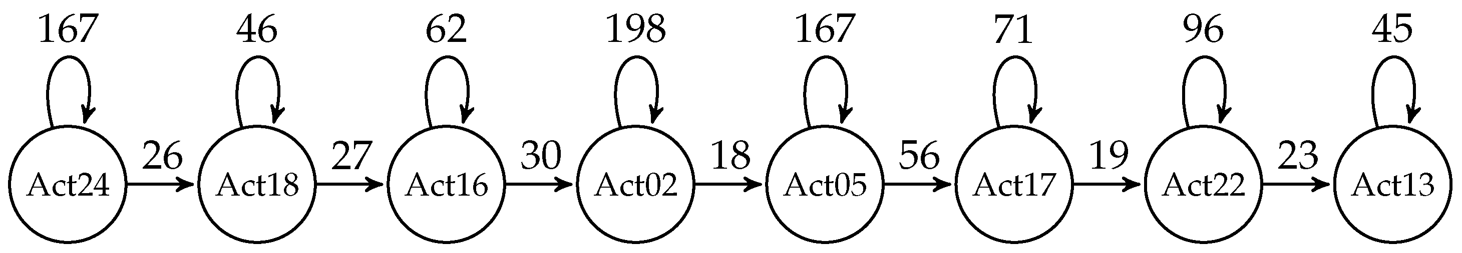
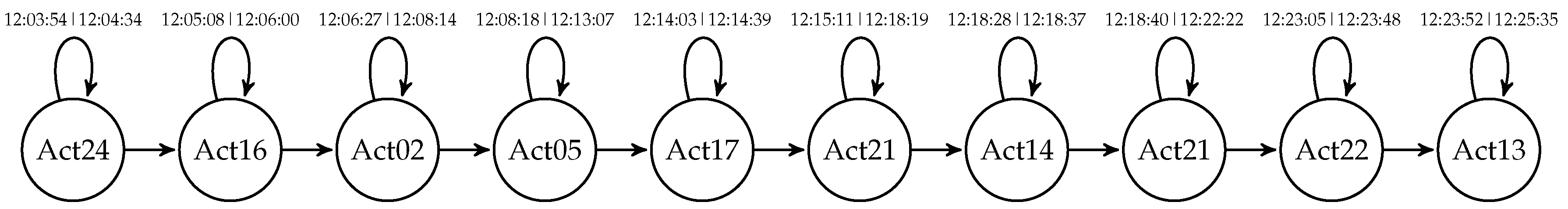
To construct the Type A automaton, we must first describe the flow of morning activities for any given day. For example, let us consider the activities recorded by the user on 31st of October in the morning, represented in

Table 2. Activities of the user.

Type: A, Date: 31 October
Act24	11:12:38	11:15:25
Act18	11:15:51	11:16:37
Act16	11:17:04	11:18:06
Act02	11:18:36	11:21:54
Act05	11:22:12	11:24:59
Act17	11:25:55	11:27:06
Act22	11:27:25	11:29:01
Act13	11:29:24	11:30:09

.

Then one can build the following graph, in which each node is an activity and the edges are labeled either with the number of seconds spent doing that particular activity or with the time elapsed between two different activities (see Figure 1).

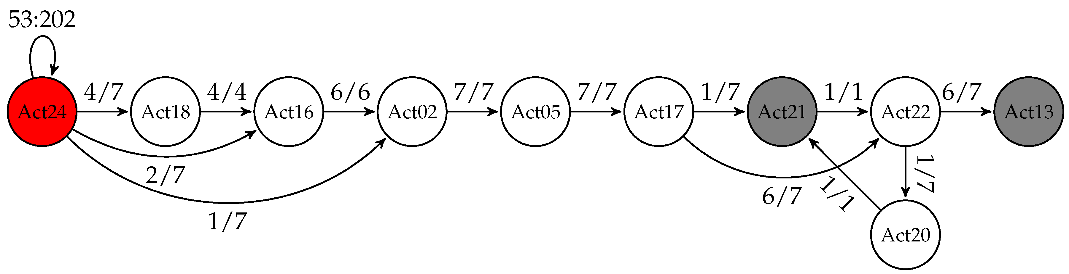
Combining activities for all available days we obtain a weighted finite automaton in which the weights indicate how many times that particular path was taken, expressed as percentage (see Figure 2).

Apart from these probabilities, we also maintain information about the minimum and maximum time spent doing each of the activities in this activity flow, as well as minimum/maximum time between two different activities (for a better readability, we chose to depict this information graphically only for one node, namely, the one representing Activity 24). Moreover, each state has a “begin” and an “end” probability (the probability of starting/finishing the morning with that particular activity). We draw in red those states that have a “begin” probability greater than zero and in gray those with non-zero “end” probabilities. Note that in the morning, the user starts his routine every day in the same way (with Activity 24: Wake up), but it may end it up either working at the table (Activity 21) or leaving the SmartLab (Activity 13).

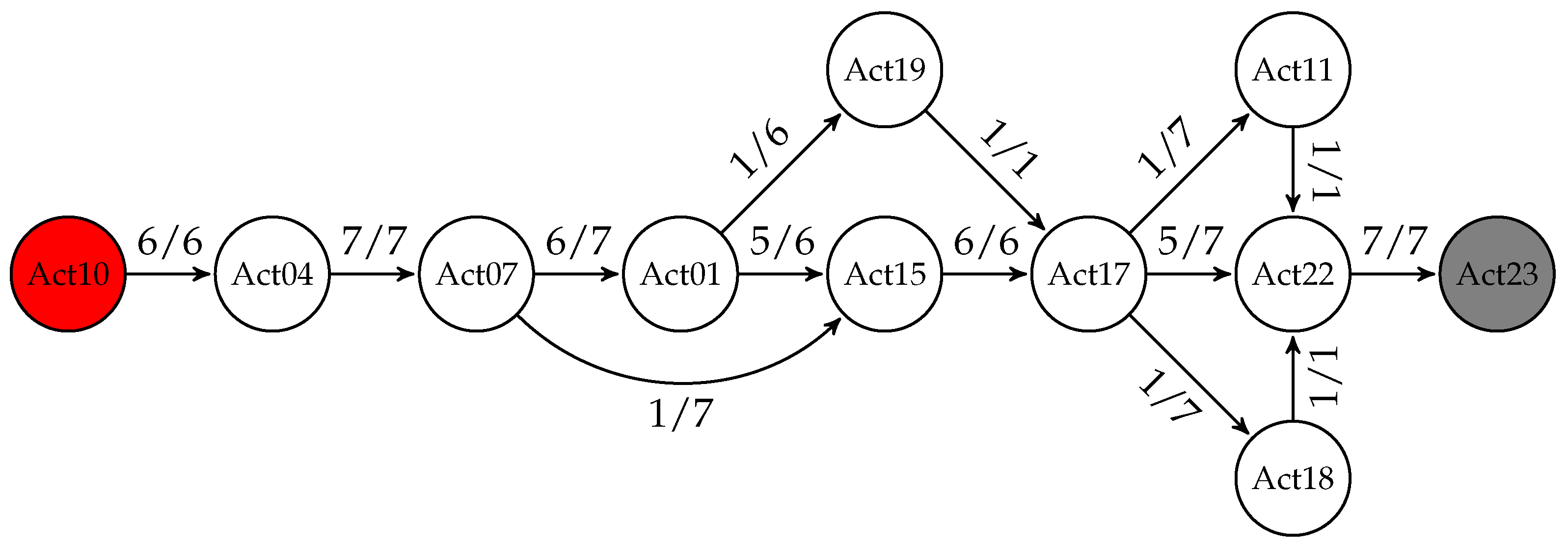
The afternoon automaton is represented in Figure 3. One can see that it is more complex than the morning one, and also that there are activities that may interrupt the normal flow, like for example, Activity 14: Visit in the SmartLab. The user may start the afternoon session either with Activity 10: Enter the SmartLab or with Activity 22: Dressing. The last activity in the afternoon is either Activity 15: Put waste in the bin (four times) or Activity 13: Leave the SmarLab (the other three times).

Finally, the evening automaton is represented in Figure 4. In this time segment, the user always started his routine with Activity 10: Enter the SmartLab and ended it with Activity 23: Go to the bed.

As we have already mentioned, we also stored, for each activity performed, the stream of sensor readings that occurred during that particular activity. In the second part of the training phase, we described by means of a regular expression each of the twenty four activities. This was a semi-supervised process. First, we learned an automaton for each activity based on the examples we had, then we converted it into a regular expression, which was eventually hand-tweaked to be more or less general, depending on our perception of how each activity should be performed.

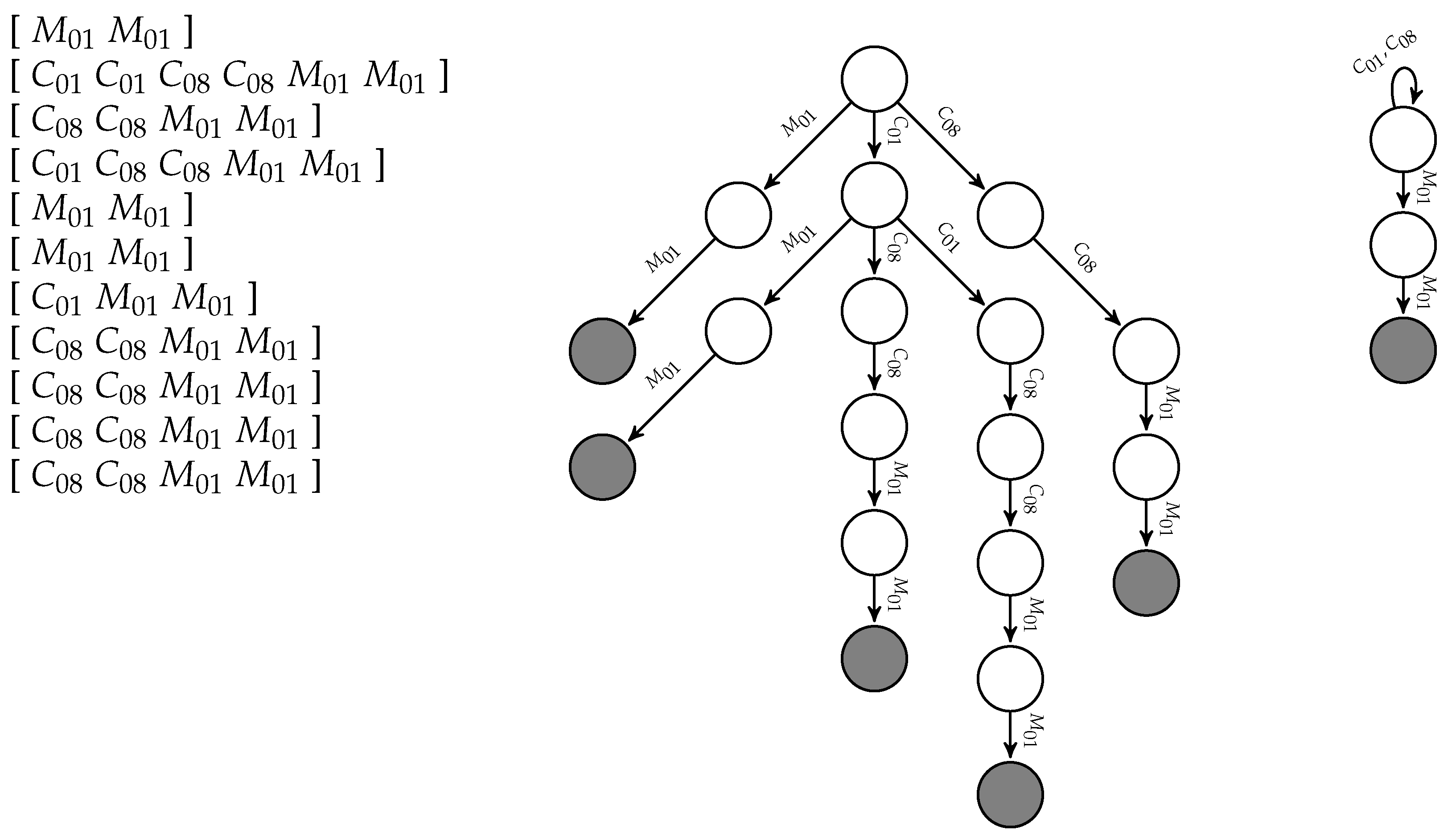
For example, the activity Put waste in the bin (Act15), which appeared eleven times in the training set, had the recordings listed in Figure 5 (left); its Prefix Tree Acceptor is depicted in Figure 5 (center), and the minimal Deterministic Finite Automaton learned by the state merging algorithm—we use a variant of the RPNI (Regular Positive and Negative Information) algorithm [15]—is represented in Figure 5 (right).

The regular expression for Put waste in the bin (Act15) is therefore ${\left(C_{01}\right|C_{08})}^{*}{M}_{01}{M}_{01}$. Note that there are only magnetic contact sensors listed in the recordings for this activity, and no motion sensor seems to be active. The reason is that we have decided to ignore those entries due to their high level of noise. We only include them whenever there is no other indication. The regular expressions obtained for each activity are listed in

Table 3. Activities’ regular expressions.

Without SM Sensors
Act01	$D_{04}^{+}(C_{01}|C_{05}|D_{04}{\left|D_{05}\right)}^{*}$	Act15	${\left(C_{01}\right|C_{08})}^{*}{M}_{01}^{+}$
Act02	$(D_{01}|D_{02}|D_{04}|D_{10}{\left|H_{01}\right)}^{+}$	Act16	$C_{09}^{+}$
Act03	$(C_{04}|D_{01}|D_{02}|D_{04}|D_{08}{\left|D_{10}\right)}^{+}$	Act17	$C_{09}^{+}$
Act04	$(C_{04}|D_{01}|D_{02}|D_{04}|D_{08}{\left|D_{10}\right)}^{+}$	Act18	${\left(C_{10}\right|D_{07})}^{+}(C_{08}|C_{10}{\left|D_{07}\right)}^{*}$
Act08	${\left(C_{02}\right|D_{10})}^{+}$	Act19	$D_{05}^{+}$
Act09	${\left(T{V}_0\right|S_{09})}^{*}T{V}_0$	Act20	$D_{09}{\left(C_{12}\right|D_{09})}^{*}$
Act10	$M_{01}^{+}$	Act22	$D_{03}(C_{12}|C_{13}{\left|D_{03}\right)}^{*}$
Act11	$\left(T{V}_0{C}_{07}\right|C_{07}T{V}_0)S_{09}^{*}\left(T{V}_0{C}_{07}\right|C_{07}T{V}_0)$	Act23	$C_{14}{\left(C_{13}\right|C_{14})}^{+}$
Act13	$M_{01}^{+}$	Act24	$C_{14}^{+}$
Act14	$M_{01}^{+}$
With SM Sensors
Act05	$S{M}_1^{+}$	Act12	$(S_{09}|S{M}_4|S{M}_5{)}^{*}S{M}_5(S_{09}|S{M}_4{\left|S{M}_5\right)}^{*}$
Act06	$S{M}_1^{+}$	Act21	$S{M}_4^{+}$
Act07	$S{M}_1^{+}$

.

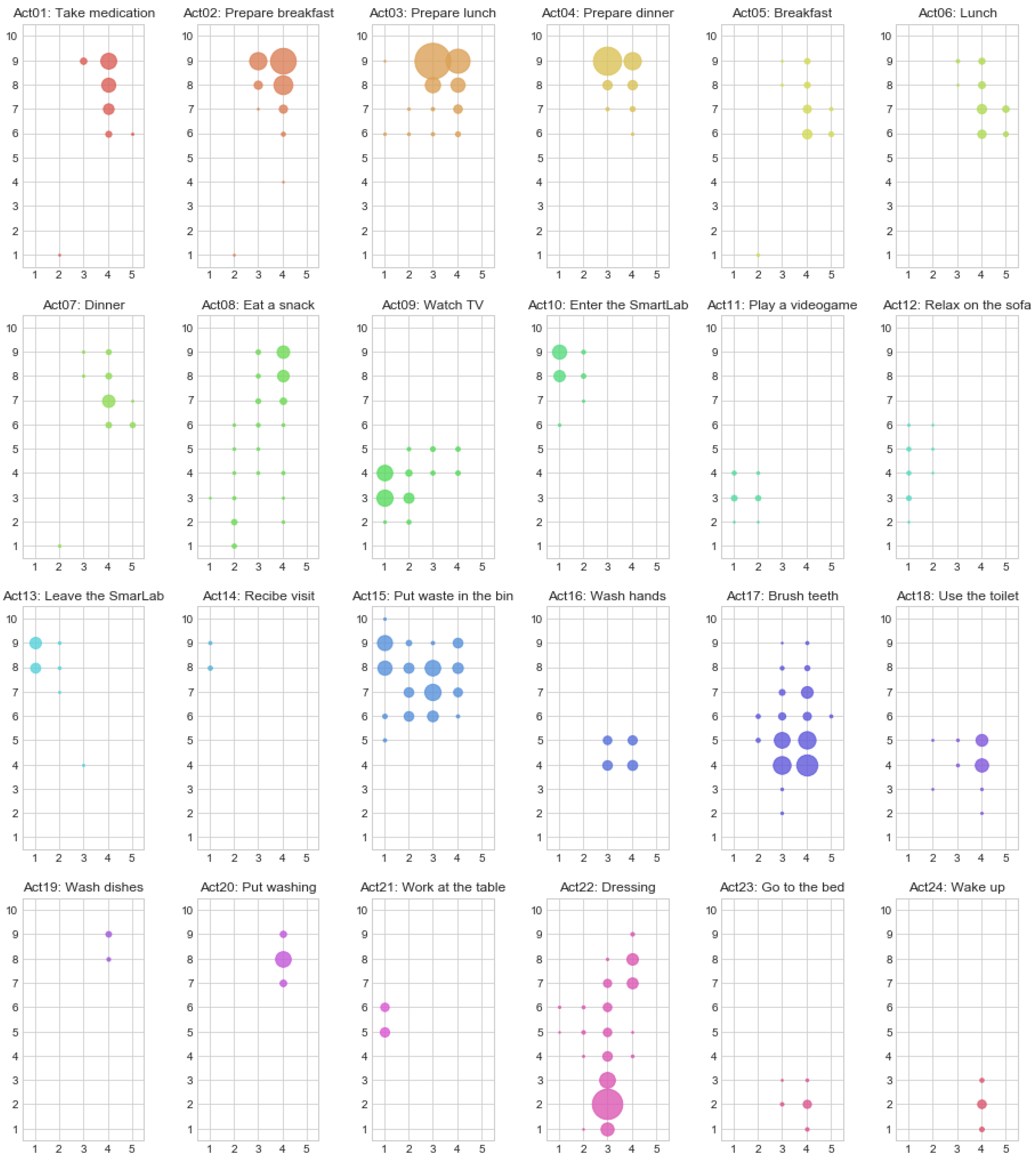
Finally, in this step we also elaborate a “map” of possible locations for each activity (using the floor capacitance information), where the radius of each point on the map depends on the occurrence frequency of that respective tile within that particular activity (we include these maps in the Appendix A of this document as Figure A1).

The set of tiles obtained for each activity will be used in the very end to fine-tune the time intervals in which each activity took place. Once we have all this information gathered, we can proceed to process the test set.

4. Prediction Step

The prediction step is also divided into two main parts. In the first one, the algorithm takes as input the sensors file of a specific routine for one particular day (for example, 2017-11-09-A-sensors.csv), and the weighted finite automaton generated for that particular routine (in this example, the one represented in Figure 2). The sensors files are mapped into the respective sequence of sensors ($S{M}_{4}S{M}_4{C}_{14}{C}_{09}S{M}_{4}S{M}_4{C}_{09}{C}_{09}{C}_{09}S{M}_1\dots$). We have implemented a filtering function that erases all motion sensors ($C_{14}{C}_{09}{C}_{09}{C}_{09}{C}_{09}\dots$). We use the unfiltered string only when necessary (basically, when the next action predicted by the automaton is Act05, Act06, Act07, Act12 or Act21), always making sure to keep track of changes in both strings.

The algorithm always tries to match first the action that has the highest probability. This holds also for the very first action, although in the morning there was only one possibility (in our example, Act24, its regular expression being $C_{14}^{+}$). Since we have a match, we save this state as the first state of the automaton, and we update both the filtered ($C_{09}{C}_{09}{C}_{09}{C}_{09}\dots$) and unfiltered ($C_{09}S{M}_{4}S{M}_4{C}_{09}\dots$) version of the sequence of sensors by erasing the matched string. The transition between this activity and itself will be labeled with provisional initial and final times, corresponding to the timestamps recorded for the first $S{M}_4$ and the last $C_{14}$ (in this case there is only one symbol, but in general the pattern may contain a whole sequence of labels), respectively. These times will be updated once we build all states and transitions of the automaton, based on the information from 2017-11-09-A-floor.csv.

The algorithm proceeds by trying to match all states with non-zero probabilities, checking first the ones with higher values (following the example, the algorithm would try first Act18, then Act16, and only if none of them matches, Act02). In this case the winner is Act16 (regular expression: $C_{09}^{+}$) since Act18 (regular expression: ${\left(C_{10}\right|D_{07})}^{+}(C_{08}|C_{10}{\left|D_{07}\right)}^{*}$) does not match the beginning of the filtered sequence of sensors.

Whenever the list of possible next states with non-zero transition probabilities is exhausted without a match, the algorithm tries, in order, what we call “unforeseen events”. These are events that can occur at any time, and they were manually selected: Act11 (Play a videogame), Act09 (Watch TV), Act14 (Visit in the SmartLab), Act18 (Use the toilet) and Act12 (Relax on the sofa). The order in which they are processed is very important in this case. Consider for example the following sequence of sensors: $T{V}_0{C}_{07}{S}_{09}{S}_{09}{S}_{09}T{V}_0{C}_{07}\dots$ Both regular expressions for Act11: $\left(T{V}_0{C}_{07}\right|C_{07}T{V}_0)S_{09}^{*}\left(T{V}_0{C}_{07}\right|C_{07}T{V}_0)$ and Act09: ${\left(T{V}_0\right|S_{09})}^{*}T{V}_0$ match the beginning of this particular string, so if the algorithm first tries with Act09, it would incorrectly predict that the user is watching TV, while the presence of the Remote XBOX ($C_{07}$) clearly indicates that the user is playing a videogame.

The next state that the algorithm tries to match after an “unforseen” event is the one that the user was performing before the interruption. If there is no match, the algorithm tries with the next activities in the workflow, starting with the most probable one. The output of this first part of the algorithm for the running example is represented by the automaton from Figure 6. One can see that after Act21, the user always performed Act22 (actually, there was only one case). But, the sequence of sensors to be matched is $M_{01}S{M}_4{M}_{01}S{M}_{4}S{M}_{4}S{M}_4\dots$, and Act22 always starts with $D_{03}$ (see its regular expression in Table 3). Since neither Act11 nor Act09 match, the algorithm proceeds to check Act14 and succeeds (for this particular activity, the filtered version of the sequence of sensors is used). Since the string left after removing the identified pattern ($S{M}_{4}S{M}_{4}S{M}_4\dots$) does match Act21, this will be the next predicted activity. If this was not the case, the algorithm would have tried with Act22.

Finally, the second part of the algorithm takes as input the automaton just produced and the corresponding floor file (2017-11-09-A-floor.csv). Each activity in the activity flow comes with some provisional initial and final times. The algorithm proceeds by updating these times based on the tiles “allowed” for that particular activity (recall that in the training phase we determine which are the possible tiles for each activity).

5. Performance Evaluation

The main goal of the 1st UCAmI Cup was to achieve the highest possible level of performance, and accuracy was the metric chosen for assessing the quality of a given solution. Our software was able to correctly identify 485 out of 535 activities, corresponding to an overall 90.65% accuracy. In

Table 4. Accuracy of our solution for each day and segment of the testing set.

	Day 1	Day 2	Day 3
Morning	43/49 (87.76%)	60/65 (92.31%)	57/59 (96.61%)
Afternoon	77/81 (95.06%)	75/79 (94.94%)	6/13 (46.15%)
Evening	57/65 (87.69%)	52/55 (94.55%)	58/69 (84.06%)

we offer detailed information about the performance obtained by our method for each day and segment of the testing set.

With one notable exception, to which we will return in Section 6, our proposed solution achieves accuracy rates between 84.06% (the evening of day 3) and 96.61% (same day, morning segment). Going through the file of results and comparing it to what our software produced, we could see that the vast majority of the errors came from having incorrectly predicted starting and ending times for our actions. There are actually only two exceptions. In one case (evening of day 1), the labeled dataset says that after dressing up (Activity 22), the inhabitant interrupted Activity 23: Go to bed to use the toilet (Activity 18): Act22-Act23-Act18-Act23, while our software found a slightly different sequence of activities: Act22-Idle-Act18-Act23. In the other case (afternoon of day 3), apart from a faulty transcription of the output of the algorithm into the excel file, both the order and the timing of half of the activities detected was completely wrong.

We would like to point out that the measure used to evaluate solutions was, in our opinion, biased. In order to justify our claim, let us clarify the way in which the final score was calculated. First, each segment of the three testing days was divided into 30 s time slots. Leaving apart technical details, participants were basically asked to fill in the list of activities (if any) that took place in each of these 30 s time slots. But, the evaluation measure only considers the first activity, adding one point to the total count if this activity was in the list of “correct” activities, and zero otherwise. Of course, a correct solution would always get one point. Unfortunately, incomplete solutions are somewhat arbitrarily rated, as we shall shortly see.

Take for example the case in which the solution given states that during a particular time slot $T_0$, ActX ends and ActY starts (see

Table 5. Time slots evaluation example.

	Solution		Labeled Test Set (Case A)		Labeled Test Set (Case B)
	ActX	ActY	ActX	ActY	ActX	ActY
Time slot $T_0$	TRUE	TRUE	TRUE	FALSE	FALSE	TRUE
Time slot $T_1$	TRUE	FALSE	TRUE	TRUE	FALSE	FALSE

). If the labeled test confirms that ActX ends indeed during time slot $T_0$ but ActY does not yet start (Case A), the event gets evaluated as correct, whereas if, according to the labeled test set, ActY did indeed start during time slot $T_0$, but activity ActX ended in a previous time slot (Case B), this event is classified as incorrect. So, in this case, it is no problem if the participant’s solution states that a certain activity started a bit earlier (Case A, ActY), but the answer is completely invalidated if a previous activity (ActX) enters, even with only one second, into the time slot that should have been allocated to the next activity (ActY) alone (Case B).

The same type of asymmetry in the evaluation process also appears in the following hypothetical situation of time slot $T_1$. If the solution states that ActY starts later than it is supposed to be (Case A), there is no problem, the event still gets one point for correctly identifying ActX ending in $T_1$. As in the case of the hypothetical situation described for Case B of time slot $T_0$, the fact that ActX takes longer than it should, would be in this case penalized in the evaluation process (Case B of time slot $T_1$).

We are aware that having to evaluate a continuous process from a discrete perspective involves by default losing precision, and that there is no perfect way around it. Nevertheless, we believe that one way to address the above mentioned inconsistencies is to consider as being correct only those time slots that coincide entirely (i.e., the list of activities returned by the solution in a given time slot is exactly the same as the list of activities in the labeled test set). Our solution would get, in this case, an overall accuracy of 87.10% (466 out of 535), with the situation per segment and day described in

Table 6. Revisited accuracy of our solution for each day and segment of the testing set.

	Day 1	Day 2	Day 3
Morning	40/49 (81.63%)	58/65 (89.23%)	54/59 (91.53%)
Afternoon	75/81 (92.59%)	74/79 (93.67%)	6/13 (46.15%)
Evening	54/65 (83.08%)	50/55 (90.91%)	55/69 (79.71%)

.

On the other hand, since for each time slot $T_i$, there is a (possibly empty) list $L_i$ of “right” or “correct” activities and a list $L_i^{\prime }$ (again, possibly empty) of activities retrieved by the participant’s solution, another possibility to evaluate the goodness of the algorithm’s output is to resort to computing true positives (activities that $L_i$ and $L_i^{\prime }$ have in common), false positives (activities in $L_i^{\prime }$ that do not appear in $L_i$) and false negatives (activities in $L_i$ that are not included in $L_i^{\prime }$), similar to what it is done in Information Retrieval. Then, one can compute an overall precision (how many of the activities found by the algorithm did indeed take place?) and recall (how many of the activities that have taken place were encountered by the algorithm?), formally defined below:

$$\mathrm{Precision}=\frac{{\sum }_i|L_i\cap L_i^{\prime }|}{{\sum }_i|L_i^{\prime }|}$$

$$\mathrm{Recall}=\frac{{\sum }_i|L_i\cap L_i^{\prime }|}{{\sum }_i|L_i|}$$

With these formulas, our solution obtains 90.72% precision (489 out of 539) and 87.95% recall (489 out of 556), amounting to a reasonably high F-measure of 0.89.

6. Conclusions and Future Work

We have implemented a Human Activity Recognizer that achieved an accuracy rate of 90.65%. Some of our mistakes are human errors introduced during the transcription process between the output file returned by our program and the csv file with results, which was done manually due to time limitations (for example, we typed Act16 instead of Act17 in 2017-11-21-B). An automatic process would therefore eliminate this problem. In other cases, we believe they are due to incorrect labeling of the test dataset. For example, for the same file, the user is supposed to be brushing his teeth between 16:10:30 and 16:12:59. Nevertheless, during that time the user is not even near the sink (according to the floor information), nor does he open or close the water tap until 16:15:34. Moreover, the bathroom motion sensor only detects movement starting at 16:15:28. Actually, the first entry in the floor file is at 16:12:51, and the first from the sensors file is at 16:13:13. And finally, there are also errors where the only ones to blame are the designers of the algorithm. We hope that by investigating the mistakes we have made, we can come up with a better software that could scale up to an arbitrary number of users and a bigger number of activities.

Another improvement that we envision is allowing more human intervention into the process. For the moment, whenever an action is longer or shorter than it is supposed to be (based on the training data), the software prints a message with this info but takes no further action. We believe that being able to stop the process when something seems to be wrong and restart it after incorporating the expert’s decision could greatly improve accuracy rates.

References

- Ranasinghe, S.; Machot, F.A.; Mayr, H.C. A review on applications of activity recognition systems with regard to performance and evaluation. Int. J. Distrib. Sens. Netw. 2016, 12. [Google Scholar] [CrossRef]
- Ann, O.C.; Theng, L.B. Human activity recognition: A review. In Proceedings of the 2014 IEEE International Conference on Control System, Computing and Engineering (ICCSCE 2014), Penang, Malaysia, 28–30 November 2014; pp. 389–393. [Google Scholar]
- Stikic, M.; Schiele, B. Activity Recognition from Sparsely Labeled Data Using Multi-Instance Learning. In Location and Context Awareness; Choudhury, T., Quigley, A., Strang, T., Suginuma, K., Eds.; Springer: Berlin/Heidelberg, Germany, 2009; pp. 156–173. [Google Scholar]
- Stiefmeier, T.; Ogris, G.; Junker, H.; Lukowicz, P.; Troster, G. Combining Motion Sensors and Ultrasonic Hands Tracking for Continuous Activity Recognition in a Maintenance Scenario. In Proceedings of the 2006 10th IEEE International Symposium on Wearable Computers, Montreux, Switzerland, 11–14 October 2006; pp. 97–104. [Google Scholar]
- Berchtold, M.; Budde, M.; Gordon, D.; Schmidtke, H.R.; Beigl, M. ActiServ: Activity Recognition Service for mobile phones. In Proceedings of the International Symposium on Wearable Computers (ISWC) 2010, Seoul, South Korea, 10–13 October 2010; pp. 1–8. [Google Scholar]
- Sefen, B.; Baumbach, S.; Dengel, A.; Abdennadher, S. Human Activity Recognition–Using Sensor Data of Smartphones and Smartwatches. In Proceedings of the 8th International Conference on Agents and Artificial Intelligence–ICAART, INSTICC, Rome, Italy, 24–26 February 2016; SciTePress, 2016; Volume 2, pp. 488–493. [Google Scholar]
- Hammerla, N.Y.; Halloran, S.; Plötz, T. Deep, Convolutional, and Recurrent Models for Human Activity Recognition Using Wearables. In Proceedings of the Twenty-Fifth International IJCAI’16, Joint Conference on Artificial Intelligence, New York, NY, USA, 9–15 July 2016; AAAI Press: Palo Alto, CA, USA, 2016; pp. 1533–1540. [Google Scholar]
- Huynh, T.; Fritz, M.; Schiele, B. Discovery of Activity Patterns Using Topic Models. In Proceedings of the 10th International Conference on Ubiquitous Computing, UbiComp ’08, Seoul, Korea, 21–24 September 2008; ACM: New York, NY, USA, 2008; pp. 10–19. [Google Scholar]
- Kwon, Y.; Kang, K.; Bae, C. Unsupervised learning for human activity recognition using smartphone sensors. Expert Syst. Appl. 2014, 41, 6067–6074. [Google Scholar] [CrossRef]
- Turaga, P.; Chellappa, R.; Subrahmanian, V.S.; Udrea, O. Machine Recognition of Human Activities: A Survey. IEEE Trans. Circuits Syst. Video Technol. 2008, 18, 1473–1488. [Google Scholar] [CrossRef]
- Lara, O.D.; Labrador, M.A. A Survey on Human Activity Recognition using Wearable Sensors. IEEE Commun. Surv. Tutor. 2013, 15, 1192–1209. [Google Scholar] [CrossRef]
- Ziaeefard, M.; Bergevin, R. Semantic human activity recognition: A literature review. Pattern Recognit. 2015, 48, 2329–2345. [Google Scholar] [CrossRef]
- Shoaib, M.; Bosch, S.; Incel, O.; Scholten, H.; Havinga, P. A Survey of Online Activity Recognition Using Mobile Phones. Sensors 2015. [Google Scholar] [CrossRef] [PubMed]
- Droste, M.; Kuich, W.; Vogler, H. Handbook of Weighted Automata, 1st ed.; Springer Publishing Company, Incorporated: Berlin, Germany, 2009. [Google Scholar]
- Oncina, J.; Garcia, P. Identifying Regular Languages In Polynomial Time. In Advances in Structural and Syntactic Pattern Recognition of Series in Machine Perception and Artificial Inteligence; World Scientific: Singapore, 1992; Volume 5, pp. 99–108. [Google Scholar]
Figure 1.
User: Mario, Date: 31 October, Type: A.
Figure 2.
User: Mario, Type: A.
Figure 3.
User: Mario, Type: B.
Figure 4.
User: Mario, Type: C.
Figure 5.
Put waste in the bin (Act15).
Figure 6.
User: Mario, Date: 19 December, Type: A.