Linearized Crank–Nicolson Scheme for the Two-Dimensional Nonlinear Riesz Space-Fractional Convection–Diffusion Equation

Abstract

In this paper, we study the nonlinear Riesz space-fractional convection–diffusion equation over a finite domain in two dimensions with a reaction term. The Crank–Nicolson difference method for the temporal and the weighted–shifted Grünwald–Letnikov difference method for the spatial discretization are proposed to achieve a second-order convergence in time and space. The D’Yakonov alternating–direction implicit technique, which is effective in two–dimensional problems, is applied to find the solution alternatively and reduce the computational cost. The unconditional stability and convergence analyses are proved theoretically. Numerical experiments with their known exact solutions are conducted to illustrate our theoretical investigation. The numerical results perfectly confirm the effectiveness and computational accuracy of the proposed method.

1. Introduction

Recently, fractional partial differential equations (FPDEs) were used to describe and model the dynamic transport of particles in porous media. Meanwhile, fractional ordinary and partial differential equations (FODEs and FPDEs) are increasingly applied in numerous fields of engineering and science, such as biology, physics, finance, chemistry, colored noise, control theory, signal processing, and so on (see the details in [1,2,3,4,5,6,7,8]). Most of the problems described by FPDEs cannot be solved analytically, so numerical approximations are becoming more important and suitable to solve these problems, such as finite volume methods [9,10], finite element methods [11,12], finite difference methods [13,14,15,16,17], spectral methods [18,19], and Galerkin methods [20,21]. The fractional space derivatives defined in the dynamical transport phenomena are commonly utilized to model the convection–diffusion equation because the particle flow distributes more rapidly than in the classical models. Moreover, the Riesz space–fractional convection–diffusion equations (RSFCDEs) have attracted increasing interest and are applied to model a wide range of real-life phenomena. As a result, the development of efficient and robust numerical techniques for RSFCDEs is an important task. Various one-dimensional RSFCDEs are solved with different numerical methods, see [15,22,23,24,25].

As we know, two–dimensional space–fractional convection–diffusion equations (2DSFCDEs) with the complexity of mathematical modeling are more challenging to find the numerical solution; therefore, the development of a simple and efficient numerical method requires more effort. Borhanifar et al. [26] combined the centered difference method with the alternating-direction implicit (ADI) finite difference scheme and derived a mixed difference approach to treat the 2DSFCD problem. Then, the convergence of the provided numerical scheme was discussed using the Lax theorem and the Lax equivalence theorem. The 2DSFCDE was solved using the ADI scheme in Chen and Deng [27] and the authors proved that the proposed finite difference method is unconditionally von Neumann stable and convergent with second order in both the time and space directions. The weighted and shifted Lubich difference operators were first introduced by Chen and Deng in [28] and then used for solving fractional diffusion equations in one- and two-dimensional space with variable coefficients. Then, the global convergence of the truncation error and unconditional stability were theoretically justified and numerically supported. A Müntz spectral technique was constructed in Hou et al. [29] for solving a class of 2DRSFCD problems and the error estimates were developed. An implicit difference method was presented in Zhou et al. [30] to find the approximation solution for the class of a two-dimensional time–space FCDE. Bi and Jiang [31] applied the finite volume element scheme with the Crank–Nicolson difference approximation to analyze the approximate solution of the 2DRSFCDE and presented their error analysis. To verify the validity of their theoretical analysis, they investigated the properties of Toplitz matrices and solved the numerical examples using the FAST–BICGSTAB algorithm.

Due to the importance of the nonlinear space-fractional convection–diffusion equations in real-world applications, some authors have developed various numerical methods to obtain the appropriate solutions. Liu et al. [32] applied the ADI approach to obtain an approximation of the solution to a two–dimensional RSFDE with homogeneous Dirichlet boundary conditions and a nonlinear source term. This numerical method was then used to simulate the 2D Riesz space–fractional Fitzhugh–Nagumo model. Zeng et al. [33] used the ADI Galerkin–Legendre spectral approach to simulate the 2DRSFDE with a nonlinear source term and extended it to treat the fractional FitzHugh–Nagumo model. Zhu et al. [34] developed the finite element algorithm that analyzes the approximate solution with the nonlinear 2D space Fisher equation such that the space derivative is based on the fractional Riesz derivative. Yang [35] investigated the numerical approximation for the RSFDE in two and three dimensions with delay and the nonlinear reaction source term using the ADI method. Then, the author developed the convergence order for the provided scheme using the Richardson extrapolation technique.

We study the following two-dimensional nonlinear Riesz space-fractional convection–diffusion equation (2DNRSFCDE):

$$\left\{\begin{array}{c}\frac{\partial \mathrm{u}(\mathrm{p},\mathrm{q},\mathrm{t})}{\partial \mathrm{t}}=-a_{\mathrm{p}}\frac{\partial \mathrm{u}(\mathrm{p},\mathrm{q},\mathrm{t})}{\partial \mathrm{p}}-a_{\mathrm{q}}\frac{\partial \mathrm{u}(\mathrm{p},\mathrm{q},\mathrm{t})}{\partial \mathrm{q}}+b_{\mathrm{p}}\frac{{\partial }^{\eta }\mathrm{u}(\mathrm{p},\mathrm{q},\mathrm{t})}{{\partial \left|\mathrm{p}\right|}^{\eta }}+b_{\mathrm{q}}\frac{{\partial }^{\sigma }\mathrm{u}(\mathrm{p},\mathrm{q},\mathrm{t})}{{\partial \left|\mathrm{q}\right|}^{\sigma }}+f(\mathrm{u},\mathrm{p},\mathrm{q},\mathrm{t}),\hfill \\ (\mathrm{p},\mathrm{q},\mathrm{t})\in \mathsf{\Omega }\times [0,T],\hfill \\ \mathrm{u}(\mathrm{p},\mathrm{q},0)=g(\mathrm{p},\mathrm{q}),(\mathrm{p},\mathrm{q})\in \mathsf{\Omega },\hfill \\ \mathrm{u}({\mathrm{p}}_l,\mathrm{q},\mathrm{t})=0,\mathrm{u}({\mathrm{p}}_r,\mathrm{q},\mathrm{t})=0,(\mathrm{q},\mathrm{t})\in [{\mathrm{q}}_l,{\mathrm{q}}_r]\times [0,T],\hfill \\ \mathrm{u}(\mathrm{p},{\mathrm{q}}_l,\mathrm{t})=0,\mathrm{u}(\mathrm{p},{\mathrm{q}}_r,\mathrm{t})=0,(\mathrm{p},\mathrm{t})\in [{\mathrm{p}}_l,{\mathrm{p}}_r]\times [0,T],\hfill \end{array}\right.$$

(1)

where $\mathrm{u}(\mathrm{p},\mathrm{q},\mathrm{t})$ is the contaminant concentration, $1<\eta ,\sigma \le 2,\mathsf{\Omega }=[{\mathrm{p}}_l,{\mathrm{p}}_r]\times [{\mathrm{q}}_l,{\mathrm{q}}_r],a_{\mathrm{p}},a_{\mathrm{q}}\ge 0$, and $b_{\mathrm{p}},b_{\mathrm{q}}>0$, represent velocity parameters and positive diffusion coefficients, respectively. f is a nonlinear function which satisfies the Lipschitz condition

$$\left|f({\mathrm{u}}_1,\mathrm{p},\mathrm{q},\mathrm{t})-f({\mathrm{u}}_2,\mathrm{p},\mathrm{q},\mathrm{t})\right|\le K|{\mathrm{u}}_1-{\mathrm{u}}_2|\forall {\mathrm{u}}_1,{\mathrm{u}}_2\in \mathbb{R},$$

(2)

where K is a Lipschitz constant.

Two–dimensional fractional PDEs are very useful to model the real-world phenomena. Therefore, the governing of a numerical solution with accurate and consistent numerical methods is necessary to make the physical meaning clear for understanding. A two–dimensional two–sided space–fractional convection–diffusion equation without a nonlinear reaction term is solved in [27] by applying the second–order accuracy alternative direction implicit (in both space and time) finite difference method. The numerical solution of the two-dimensional Riesz space–fractional nonlinear reaction–diffusion equation was considered by [33] using the Crank–Nicolson ADI Galerkin–Legendre spectral method. The proposed method is conditionally stable with the convergence of second order in time and an optimal error estimate in space. The numerical approximate solution of the nonlinear space-fractional reaction–diffusion equation was constructed by [32]. They used the alternative direction implicit finite difference method combined with the shifted Grünwald–Letnikov difference scheme to produce the first order in both space and time. In this paper, the theoretical analysis and numerical computation of the two–dimensional nonlinear Risez space–fractional convection–diffusion equation on a finite domain are considered. We propose a second order in time Crank–Nicolson ADI difference method combined with a second order in space weighted–shifted Grünwald–Letnikov difference (WSGD) technique to find the numerical solution of the problem in two dimensions which improve the spatial and temporal accuracy with the presence of a nonlinear term. Because using a fixed-point iteration method to obtain an approximation solution of a nonlinear system of equations for each of the time steps requires a lot of computing power, we have linearized our problem. The Lipschitz condition is satisfied by the nonlinear function, and the theoretical examination of the stability and convergence analysis demonstrates that the CNADI–WSGD method is unconditionally stable and convergent in time and space with second-order accuracy.

The remaining sections of the paper are organized as follows: Section 2 presents some basic definitions and preliminary lemmas. The CNADI–WSGD scheme is proposed and formulated in Section 3 for the two–dimensional nonlinear Riesz space–fractional convection–diffusion problem (1). The stability and consistency analysis of the problem is discussed theoretically in Section 4. In Section 5, we perform the numerical experiments with exact solutions that confirm the theoretical analysis of the implemented problem. In Section 6, a conclusion is drawn based on the obtained results.

2. Preliminaries

We give in this section important key concepts, lemmas, and notations that will be useful as the work develops.

Definition 1 

([36]). The fractional derivatives of Riesz with orders $\eta ,\sigma (m-1<\eta ,\sigma \le m)$ of the function $\mathrm{u}(\mathrm{p},\mathrm{q},\mathrm{t})$ in a finite domain $[{\mathrm{p}}_l,{\mathrm{p}}_r]\times [{\mathrm{q}}_l,{\mathrm{q}}_r]$ are defined as

$$\frac{{\partial }^{\eta }\mathrm{u}(\mathrm{p},\mathrm{q},\mathrm{t})}{{\partial \left|\mathrm{p}\right|}^{\eta }}=-{\kappa }_{\eta }\{{}_{{\mathrm{p}}_l}{D}_{\mathrm{p}}^{\eta }\mathrm{u}(\mathrm{p},\mathrm{q},\mathrm{t})+{}_{\mathrm{p}}{D}_{{\mathrm{p}}_r}^{\eta }\mathrm{u}(\mathrm{p},\mathrm{q},\mathrm{t})\},$$

$$\frac{{\partial }^{\sigma }\mathrm{u}(\mathrm{p},\mathrm{q},\mathrm{t})}{{\partial \left|\mathrm{p}\right|}^{\sigma }}=-{\kappa }_{\sigma }\{{}_{{\mathrm{q}}_l}{D}_{\mathrm{q}}^{\sigma }\mathrm{u}(\mathrm{p},\mathrm{q},\mathrm{t})+{}_{\mathrm{q}}{D}_{{\mathrm{q}}_r}^{\sigma }\mathrm{u}(\mathrm{p},\mathrm{q},\mathrm{t})\},$$

where ${\kappa }_{\eta }=\frac{1}{2cos\frac{\pi \eta }{2}},{\kappa }_{\sigma }=\frac{1}{2cos\frac{\pi \sigma }{2}},\eta ,\sigma \ne 1$.

Definition 2 

([37]). For a smooth function $\mathrm{u}(\mathrm{p},\mathrm{q},\mathrm{t})$, the left–sided and right–sided Riemann–Liouville (RL) space-fractional derivatives with orders $\eta ,\sigma (m-1<\eta ,\sigma \le m)$ on the finite domain $[{\mathrm{p}}_l,{\mathrm{p}}_r]\times [{\mathrm{q}}_l,{\mathrm{q}}_r]$ are defined, respectively, as

$${}_{{\mathrm{p}}_l}{D}_{\mathrm{p}}^{\eta }\mathrm{u}(\mathrm{p},\mathrm{q},\mathrm{t})=\frac{1}{\mathsf{\Gamma }(m-\eta )}\frac{d^m}{d{\mathrm{p}}^m}{\int }_{{\mathrm{p}}_l}^{\mathrm{p}}\frac{\mathrm{u}(\vartheta ,\mathrm{q},\mathrm{t})}{{(\mathrm{u}-\vartheta )}^{\eta -m+1}}d\vartheta ,$$

$${}_{\mathrm{p}}{D}_{{\mathrm{p}}_r}^{\eta }\mathrm{u}(\mathrm{p},\mathrm{q},\mathrm{t})=\frac{{(-1)}^m}{\mathsf{\Gamma }(m-\eta )}\frac{d^m}{d{\mathrm{p}}^m}{\int }_{\mathrm{p}}^{{\mathrm{p}}_r}\frac{\mathrm{u}(\vartheta ,\mathrm{q},\mathrm{t})}{{(\vartheta -\mathrm{u})}^{\eta -m+1}}d\vartheta ,$$

in which $\mathsf{\Gamma }(.)$ denotes the Euler gamma function.

The left–sided and right-sided Riemann–Liouville fractional derivatives in q–direction can be defined similarly.

Definition 3 

([38]). The Grünwald–Letnikov (GL) formula for the left-sided and right-sided fractional derivatives on the finite domain $[{\mathrm{p}}_l,{\mathrm{p}}_r]\times [{\mathrm{q}}_l,{\mathrm{q}}_r]$ are, respectively, given by

$${}_{{\mathrm{p}}_l}{D}_{\mathrm{p}}^{\eta }\mathrm{u}(\mathrm{p},\mathrm{q})=\underset{h_{\mathrm{p}}\to 0^{+}}{lim}\frac{1}{h_{\mathrm{p}}^{\eta }}\sum _{\theta =0}^{\frac{(\mathrm{p}-{\mathrm{p}}_l)}{h}}{(-1)}^{\theta }\left(\begin{array}{c}\eta \hfill \\ \theta \hfill \end{array}\right)\mathrm{u}(\mathrm{p}-\theta h_{\mathrm{p}},\mathrm{q}),$$

$${}_{\mathrm{p}}{D}_{{\mathrm{p}}_r}^{\eta }\mathrm{u}(\mathrm{p},\mathrm{q})=\underset{h_{\mathrm{p}}\to 0^{+}}{lim}\frac{1}{h_{\mathrm{p}}^{\eta }}\sum _{\theta =0}^{\frac{({\mathrm{p}}_r-\mathrm{p})}{h}}{(-1)}^{\theta }\left(\begin{array}{c}\eta \hfill \\ \theta \hfill \end{array}\right)\mathrm{u}(\mathrm{p}+\theta h_{\mathrm{p}},\mathrm{q}).$$

Similarly, the (GL) formula for the left-sided and right-sided fractional derivatives with respect to $\mathrm{q}$-direction on the finite interval $[{\mathrm{q}}_l,{\mathrm{q}}_r]$ is defined as

$${}_{{\mathrm{q}}_l}{D}_{\mathrm{q}}^{\sigma }\mathrm{u}(\mathrm{p},\mathrm{q})=\underset{h_{\mathrm{q}}\to 0^{+}}{lim}\frac{1}{h_{\mathrm{q}}^{\sigma }}\sum _{\theta =0}^{\frac{(\mathrm{q}-{\mathrm{q}}_l)}{h}}{(-1)}^{\theta }\left(\begin{array}{c}\sigma \hfill \\ \theta \hfill \end{array}\right)\mathrm{u}(\mathrm{p},\mathrm{q}-\theta h_{\mathrm{q}}),$$

$${}_{\mathrm{q}}{D}_{{\mathrm{q}}_r}^{\sigma }\mathrm{u}(\mathrm{p},\mathrm{q})=\underset{h_{\mathrm{q}}\to 0^{+}}{lim}\frac{1}{h_{\mathrm{q}}^{\sigma }}\sum _{\theta =0}^{\frac{({\mathrm{q}}_r-\mathrm{q})}{h}}{(-1)}^{\theta }\left(\begin{array}{c}\sigma \hfill \\ \theta \hfill \end{array}\right)\mathrm{u}(\mathrm{p},\mathrm{q}+\theta h_{\mathrm{q}}).$$

If $\mathrm{u}(\mathrm{p},\mathrm{q})$ is defined on the finite interval $[{\mathrm{p}}_l,{\mathrm{p}}_r]\times [{\mathrm{q}}_l,{\mathrm{q}}_r]$ and $\mathrm{u}({\mathrm{p}}_l,\mathrm{q})=\mathrm{u}({\mathrm{p}}_r,\mathrm{q})=\mathrm{u}(\mathrm{p},{\mathrm{q}}_l)=\mathrm{u}(\mathrm{p},{\mathrm{q}}_r)=0$, then the function $\mathrm{u}(\mathrm{p},\mathrm{q})$ can be zero-extended for $\mathrm{p}<{\mathrm{p}}_l,\mathrm{q}<{\mathrm{q}}_l$ or $\mathrm{p}>{\mathrm{p}}_r,\mathrm{q}>{\mathrm{q}}_r$. Let us suppose that the function $\mathrm{u}(\mathrm{p},\mathrm{q})$ is $m-1$-continuously differentiable in the intervals $[{\mathrm{p}}_l,{\mathrm{p}}_r],[{\mathrm{q}}_l,{\mathrm{q}}_r]$ and that ${\mathrm{u}}^{\left(m\right)}(\mathrm{p},\mathrm{q})$ is integrable in $[{\mathrm{p}}_l,{\mathrm{p}}_r],[{\mathrm{q}}_l,{\mathrm{q}}_r]$. Then, for every $\eta ,\sigma (0\le m-1\le \eta ,\sigma \le m)$, the RL fractional derivative exists and coincides with the GL fractional derivative [39]. The GL and the RL derivatives are equivalent for a sufficiently smooth function, as showed in [40]. The GL approximation is frequently applied to numerically estimate the RL derivative and was the first approach to arise for approximating fractional derivatives. In particular, the shifted Grünwald difference operator is given as [41]

$$\begin{array}{cc}\hfill & A_{+\mathrm{p},r}^{\eta }\mathrm{u}(\mathrm{p},\mathrm{q})=\frac{1}{h_{\mathrm{p}}^{\eta }}\sum _{\theta =0}^{\infty }{\mathrm{g}}_{\theta }^{\left(\eta \right)}\mathrm{u}(\mathrm{p}-(\theta -r)h_{\mathrm{p}},\mathrm{q}),\hfill \\ \hfill & B_{-\mathrm{p},r}^{\eta }\mathrm{u}(\mathrm{p},\mathrm{q})=\frac{1}{h_{\mathrm{p}}^{\eta }}\sum _{\theta =0}^{\infty }{\mathrm{g}}_{\theta }^{\left(\eta \right)}\mathrm{u}(\mathrm{p}+(\theta -r)h_{\mathrm{p}},\mathrm{q}),\hfill \end{array}$$

(3)

$$\begin{array}{cc}\hfill & A_{+\mathrm{q},r}^{\sigma }\mathrm{u}(\mathrm{p},\mathrm{q})=\frac{1}{h_{\mathrm{q}}^{\sigma }}\sum _{\theta =0}^{\infty }{\mathrm{g}}_{\theta }^{\left(\sigma \right)}\mathrm{u}(\mathrm{p},\mathrm{q}-(\theta -r)h_{\mathrm{q}}),\hfill \\ \hfill & B_{-\mathrm{q},r}^{\sigma }\mathrm{u}(\mathrm{p},\mathrm{q})=\frac{1}{h_{\mathrm{q}}^{\sigma }}\sum _{\theta =0}^{\infty }{\mathrm{g}}_{\theta }^{\left(\sigma \right)}\mathrm{u}(\mathrm{p},\mathrm{q}+(\theta -r)h_{\mathrm{q}}),\hfill \end{array}$$

(4)

approximating both the left and right RL fractional derivatives which give first–order convergence, i.e.,

$$\begin{array}{cc}\hfill & A_{+\mathrm{p},r}^{\eta }\mathrm{u}(\mathrm{p},\mathrm{q})={}_{-\infty }{D}_{\mathrm{p}}^{\eta }\mathrm{u}(\mathrm{p},\mathrm{q})+\mathcal{O}\left(h_{\mathrm{p}}\right),\hfill \\ \hfill & B_{-\mathrm{p},r}^{\eta }\mathrm{u}(\mathrm{p},\mathrm{q})={}_{\mathrm{p}}{D}_{+\infty }^{\eta }\mathrm{u}(\mathrm{p},\mathrm{q})+\mathcal{O}\left(h_{\mathrm{p}}\right),\hfill \end{array}$$

(5)

$$\begin{array}{cc}\hfill & A_{+\mathrm{q},r}^{\sigma }\mathrm{u}(\mathrm{p},\mathrm{q})={}_{-\infty }{D}_{\mathrm{q}}^{\sigma }\mathrm{u}(\mathrm{p},\mathrm{q})+\mathcal{O}\left(h_{\mathrm{q}}\right),\hfill \\ \hfill & B_{-\mathrm{q},r}^{\sigma }\mathrm{u}(\mathrm{p},\mathrm{q})={}_{\mathrm{q}}{D}_{+\infty }^{\sigma }\mathrm{u}(\mathrm{p},\mathrm{q})+\mathcal{O}\left(h_{\mathrm{q}}\right),\hfill \end{array}$$

(6)

where r is a positive integer and ${\mathrm{g}}_{\theta }^{\left(\eta \right)}={(-1)}^{\theta }\left(\begin{array}{c}\eta \hfill \\ \theta \hfill \end{array}\right)$ are the power series coefficients for the generating function ${(1-z)}^{\eta }$,

$${(1-z)}^{\eta }=\sum _{\theta =0}^{\infty }{(-1)}^{\theta }\left(\begin{array}{c}\eta \hfill \\ \theta \hfill \end{array}\right)z^{\theta }=\sum _{\theta =0}^{\infty }{\mathrm{g}}_{\theta }^{\left(\eta \right)}{z}^{\theta },$$

(7)

for all $\left|z\right|\le 1$, and they can be derived successively:

$${\mathrm{g}}_0^{\left(\eta \right)}=1,{\mathrm{g}}_{\theta }^{\left(\eta \right)}=\left(1-\frac{\eta +1}{\theta }\right){\mathrm{g}}_{\theta -1}^{\left(\eta \right)},\theta =1,2,\dots .$$

(8)

Lemma 1 

([42]). For the fractional order $1<\eta \le 2$, the coefficients in Equation (4) satisfy the properties shown below.

$$\left\{\begin{array}{c}{\mathrm{g}}_0^{\left(\eta \right)}=1,{\mathrm{g}}_1^{\left(\eta \right)}=-\eta <0,\hfill \\ 1\ge {\mathrm{g}}_2^{\left(\eta \right)}\ge {\mathrm{g}}_3^{\left(\eta \right)}\ge \dots \ge 0,\hfill \\ \sum _{\theta =0}^{\infty }{\mathrm{g}}_{\theta }^{\left(\eta \right)}=0,\sum _{\theta =0}^{N_{\mathrm{p}}}{\mathrm{g}}_{\theta }^{\left(\eta \right)}<0,N_{\mathrm{p}}\ge 1.\hfill \end{array}\right.$$

(9)

The left and right RL fractional derivatives for the continuous function $\mathrm{u}(\mathrm{p},\mathrm{q})$ at every point ${\mathrm{p}}_{\nu },{\mathrm{q}}_{\upsilon },\nu =1,2,...,N_{\mathrm{p}},\upsilon =1,2,...,N_{\mathrm{q}}$ on a finite interval $[{\mathrm{p}}_l,{\mathrm{p}}_r],[{\mathrm{q}}_l,{\mathrm{q}}_r]$, which is using the weighted and shifted GL formula, can be written as follows:

$$\begin{array}{cc}\hfill & {}_{{\mathrm{p}}_l}{D}_{\mathrm{p}}^{\eta }\mathrm{u}({\mathrm{p}}_{\nu },{\mathrm{q}}_{\upsilon })=\frac{1}{h_{\mathrm{p}}^{\eta }}\sum _{\theta =0}^{\nu +1}{\omega }_{\theta }^{\eta }\mathrm{u}(\nu -\theta +1,\upsilon )+\mathcal{O}\left(h_{\mathrm{p}}^2\right),\hfill \\ \hfill & {}_{\mathrm{p}}{D}_{{\mathrm{p}}_r}^{\eta }\mathrm{u}({\mathrm{p}}_{\nu },{\mathrm{q}}_{\upsilon })=\frac{1}{h_{\mathrm{p}}^{\eta }}\sum _{\theta =0}^{N_{\mathrm{p}}-\nu +1}{\omega }_{\theta }^{\eta }\mathrm{u}(\nu +\theta -1,\upsilon )+\mathcal{O}\left(h_{\mathrm{p}}^2\right),\hfill \end{array}$$

(10)

in which

$${\omega }_0^{\left(\eta \right)}=\frac{\eta }{2}{\mathrm{g}}_0^{\left(\eta \right)},{\omega }_{\theta }^{\left(\eta \right)}=\frac{\eta }{2}{\mathrm{g}}_{\theta }^{\left(\eta \right)}+\frac{2-\eta }{2}{\mathrm{g}}_{\theta -1}^{\left(\eta \right)}\mathrm{for}\theta \ge 1.$$

The definition of the weighted and shifted GL formula for the $\mathrm{q}$-direction is the same as Equation (10).

Lemma 2 

([41]). For the fractional order $1<\eta \le 2$, the coefficients in (10) satisfy the following properties:

$$\left\{\begin{array}{c}{\omega }_0^{\left(\eta \right)}=\frac{\eta }{2}>0,{\omega }_1^{\left(\eta \right)}=\frac{2-\eta -{\eta }^2}{2}<0,{\omega }_2^{\left(\eta \right)}=\frac{\eta ({\eta }^2+\eta -4)}{4},\hfill \\ 1\ge {\omega }_0^{\left(\eta \right)}\ge {\omega }_3^{\left(\eta \right)}\ge {\omega }_4^{\left(\eta \right)}\ge \dots \ge 0,\hfill \\ \sum _{\theta =0}^{\infty }{\omega }_{\theta }^{\left(\eta \right)}=0,\sum _{\theta =0}^{N_{\mathrm{p}}}{\omega }_{\theta }^{\left(\eta \right)}<0,N_{\mathrm{p}}\ge 2.\hfill \end{array}\right.$$

(11)

3. CNADI-WSGD Method

In this part, we show an approximate numerical solution to problem (1). Let $\mathsf{\Omega }=[{\mathrm{p}}_l,{\mathrm{p}}_r]\times [{\mathrm{q}}_l,{\mathrm{q}}_r]$ be a finite domain, and let $h_{\mathrm{p}}=({\mathrm{p}}_r-{\mathrm{p}}_l)/N_{\mathrm{p}}$ with ${\mathrm{p}}_{\nu }={\mathrm{p}}_l+\nu h_{\mathrm{p}}$ for $\nu =0,1,2,...,N_{\mathrm{p}},$$h_{\mathrm{q}}=({\mathrm{q}}_r-{\mathrm{q}}_l)/N_{\mathrm{q}}$ with ${\mathrm{q}}_{\upsilon }={\mathrm{q}}_l+\upsilon h_{\mathrm{q}}$ for $\upsilon =0,1,2,...,N_{\mathrm{q}}$ are the spatial grid size in the x–direction and the spatial grid size in the y–direction, respectively. Let $\tau =T/N_{\mathrm{t}}$ be the time step with partition ${\mathrm{t}}_n=n\tau$, for $n=0,1,2,...,N_{\mathrm{t}}$, where $N_{\mathrm{p}},N_{\mathrm{q}},N_{\mathrm{t}}$ are nonnegative integers. The Crank–Nicolson scheme and the WSGD formula are used for the temporal and spatial discretizations, respectively. The convection term in (1) is also approximated by the central finite difference method. Define ${\mathrm{u}}_{\nu ,\upsilon }^n$ as the numerical approximation to $\mathrm{u}({\mathrm{p}}_{\nu },{\mathrm{q}}_{\upsilon },{\mathrm{t}}_n),{\mathrm{t}}_{n+\frac{1}{2}}=\frac{({\mathrm{t}}_n+{\mathrm{t}}_{n+1})}{2},f\left({\mathrm{u}}^{n+\frac{1}{2}}\right)=f({\mathrm{u}}_{\nu ,\upsilon }^{n+\frac{1}{2}},{\mathrm{p}}_{\nu },{\mathrm{q}}_{\upsilon },{\mathrm{t}}_{n+\frac{1}{2}})$. For the uniform time step $\tau$ and the space steps $h_{\mathrm{p}},h_{\mathrm{q}}$, the resulting discretization of (1) can be formulated as

$$\begin{array}{ccc}\hfill & & \frac{{\mathrm{u}}_{\nu ,\upsilon }^{n+1}-{\mathrm{u}}_{\nu ,\upsilon }^n}{\tau }=\frac{-a_{\mathrm{p}}}{2}\frac{\left({\mathrm{u}}_{\nu +1,\upsilon }^{n+1}-{\mathrm{u}}_{\nu -1,\upsilon }^{n+1}+{\mathrm{u}}_{\nu +1,\upsilon }^n-{\mathrm{u}}_{\nu -1,\upsilon }^n\right)}{2h_{\mathrm{p}}}+\frac{-a_{\mathrm{q}}}{2}\frac{\left({\mathrm{u}}_{\nu ,\upsilon +1}^{n+1}-{\mathrm{u}}_{\nu ,\upsilon -1}^{n+1}+{\mathrm{u}}_{\nu ,\upsilon +1}^n-{\mathrm{u}}_{\nu ,\upsilon -1}^n\right)}{2h_{\mathrm{q}}}\hfill \\ & -& \frac{{\kappa }_{\eta }{b}_{\mathrm{p}}}{2h_{\mathrm{p}}^{\eta }}\left(\sum _{\theta =0}^{\nu +1}{\omega }_{\theta }^{\left(\eta \right)}{\mathrm{u}}_{\nu -\theta +1,\upsilon }^{n+1}+\sum _{\theta =0}^{N_{\mathrm{p}}-\nu +1}{\omega }_{\theta }^{\left(\eta \right)}{\mathrm{u}}_{\nu +\theta -1,\upsilon }^{n+1}+\sum _{\theta =0}^{\nu +1}{\omega }_{\theta }^{\left(\eta \right)}{\mathrm{u}}_{\nu -\theta +1,\upsilon }^n+\sum _{\theta =0}^{N_{\mathrm{p}}-\nu +1}{\omega }_{\theta }^{\left(\eta \right)}{\mathrm{u}}_{\nu +\theta -1,\upsilon }^n\right)\hfill \\ & -& \frac{{\kappa }_{\sigma }{b}_{\mathrm{q}}}{2h_{\mathrm{q}}^{\sigma }}\left(\sum _{\theta =0}^{\upsilon +1}{\omega }_{\theta }^{\left(\sigma \right)}{\mathrm{u}}_{\nu ,\upsilon -\theta +1}^{n+1}+\sum _{\theta =0}^{N_{\mathrm{q}}-\upsilon +1}{\omega }_{\theta }^{\left(\sigma \right)}{\mathrm{u}}_{\nu ,\upsilon +\theta -1}^{n+1}+\sum _{\theta =0}^{\upsilon +1}{\omega }_{\theta }^{\left(\sigma \right)}{\mathrm{u}}_{\nu ,\upsilon -\theta +1}^n+\sum _{\theta =0}^{N_{\mathrm{q}}-\upsilon +1}{\omega }_{\theta }^{\left(\sigma \right)}{\mathrm{u}}_{\nu ,\upsilon +\theta -1}^n\right)\hfill \\ & +& f({\mathrm{u}}_{\nu ,\upsilon }^{n+\frac{1}{2}},{\mathrm{p}}_{\nu },{\mathrm{q}}_{\upsilon },{\mathrm{t}}_{n+\frac{1}{2}}),\hfill \end{array}$$

(12)

where ${\kappa }_{\eta }=\frac{1}{2cos(\pi \eta /2)},{\kappa }_{\sigma }=\frac{1}{2cos(\pi \sigma /2)}$. Thus, the weighted–shifted Grünwald difference method with Crank–Nicolson finite difference for problem (1) is expressed as

$$\begin{array}{ccc}\hfill & & {\mathrm{u}}_{\nu ,\upsilon }^{n+1}+\frac{{\overline{a}}_{\mathrm{p}}}{2}\left({\mathrm{u}}_{\nu +1,\upsilon }^{n+1}-{\mathrm{u}}_{\nu -1,\upsilon }^{n+1}\right)+\frac{{\overline{a}}_{\mathrm{q}}}{2}\left({\mathrm{u}}_{\nu ,\upsilon +1}^{n+1}-{\mathrm{u}}_{\nu ,\upsilon -1}^{n+1}\right)\hfill \\ & +& \frac{{\overline{b}}_{\mathrm{p}}}{2}\left(\sum _{\theta =0}^{\nu +1}{\omega }_{\theta }^{\left(\eta \right)}{\mathrm{u}}_{\nu -\theta +1,\upsilon }^{n+1}+\sum _{\theta =0}^{N_{\mathrm{p}}-\nu +1}{\omega }_{\theta }^{\left(\eta \right)}{\mathrm{u}}_{\nu +\theta -1,\upsilon }^{n+1}\right)\hfill \\ & +& \frac{{\overline{b}}_{\mathrm{q}}}{2}\left(\sum _{\theta =0}^{\upsilon +1}{\omega }_{\theta }^{\left(\sigma \right)}{\mathrm{u}}_{\nu ,\upsilon -\theta +1}^{n+1}+\sum _{\theta =0}^{N_{\mathrm{q}}-\nu +1}{\omega }_{\theta }^{\left(\sigma \right)}{\mathrm{u}}_{\nu ,\upsilon +\theta -1}^{n+1}\right)\hfill \\ & =& {\mathrm{u}}_{\nu ,\upsilon }^n-\frac{{\overline{a}}_{\mathrm{p}}}{2}\left({\mathrm{u}}_{\nu -1,\upsilon }^n-{\mathrm{u}}_{\nu +1,\upsilon }^n\right)+\frac{{\overline{a}}_{\mathrm{q}}}{2}\left({\mathrm{u}}_{\nu ,\upsilon -1}^n-{\mathrm{u}}_{\nu ,\upsilon +1}^n\right)\hfill \\ & -& \frac{{\overline{b}}_{\mathrm{p}}}{2}\left(\sum _{\theta =0}^{\nu +1}{\omega }_{\theta }^{\left(\eta \right)}{\mathrm{u}}_{\nu -\theta +1,\upsilon }^n+\sum _{\theta =0}^{N_{\mathrm{p}}-\nu +1}{\omega }_{\theta }^{\left(\eta \right)}{\mathrm{u}}_{\nu +\theta -1,\upsilon }^n\right)\hfill \\ & -& \frac{{\overline{b}}_{\mathrm{q}}}{2}\left(\sum _{\theta =0}^{\upsilon +1}{\omega }_{\theta }^{\left(\sigma \right)}{\mathrm{u}}_{\nu ,\upsilon -\theta +1}^n+\sum _{\theta =0}^{N_{\mathrm{q}}-\upsilon +1}{\omega }_{\theta }^{\left(\sigma \right)}{\mathrm{u}}_{\nu ,\upsilon +\theta -1}^n\right)\hfill \\ & +& \tau f({\mathrm{u}}_{\nu ,\upsilon }^{n+\frac{1}{2}},{\mathrm{p}}_{\nu },{\mathrm{q}}_{\upsilon },{\mathrm{t}}_{n+\frac{1}{2}}),\hfill \end{array}$$

(13)

where ${\overline{a}}_{\mathrm{p}}=\frac{\tau a_{\mathrm{p}}}{2h_{\mathrm{p}}},{\overline{b}}_{\mathrm{p}}=\frac{\tau {\kappa }_{\eta }{b}_{\mathrm{p}}}{h_{\mathrm{p}}^{\eta }},{\overline{a}}_{\mathrm{q}}=\frac{\tau a_{\mathrm{q}}}{2h_{\mathrm{q}}},{\overline{b}}_{\mathrm{q}}=\frac{\tau {\kappa }_{\sigma }{b}_{\mathrm{q}}}{h_{\mathrm{q}}^{\sigma }}$. Define the following operators to simplify our formulation

$$\begin{array}{cc}\hfill & {\delta }_{\mathrm{p}}^{\prime }{\mathrm{u}}_{\nu ,\upsilon }^n=\frac{-a_{\mathrm{p}}({\mathrm{u}}_{\nu +1,\upsilon }^n-{\mathrm{u}}_{\nu -1,\upsilon }^n)}{2h_{\mathrm{p}}},{\delta }_{\mathrm{q}}^{\prime }{\mathrm{u}}_{\nu ,\upsilon }^n=\frac{-a_{\mathrm{q}}({\mathrm{u}}_{\nu ,\upsilon +1}^n-{\mathrm{u}}_{\nu ,\upsilon -1}^n)}{2h_{\mathrm{q}}},\hfill \\ \hfill & {\delta }_{\mathrm{p}}^{\eta }{\mathrm{u}}_{\nu ,\upsilon }^n=-\frac{{\kappa }_{\eta }{b}_{\mathrm{p}}}{h_{\mathrm{p}}^{\eta }}\left(\sum _{\theta =0}^{\nu +1}{\omega }_{\theta }^{\left(\eta \right)}{\mathrm{u}}_{\nu -\theta +1,\upsilon }^n+\sum _{\theta =0}^{N_{\mathrm{p}}-\nu +1}{\omega }_{\theta }^{\left(\eta \right)}{\mathrm{u}}_{\nu +\theta -1,\upsilon }^n\right)+\mathcal{O}\left(h_{\mathrm{p}}^2\right),\hfill \\ \hfill & {\delta }_{\mathrm{q}}^{\sigma }{\mathrm{u}}_{\nu ,\upsilon }^n=-\frac{{\kappa }_{\sigma }{b}_{\mathrm{q}}}{h_{\mathrm{q}}^{\sigma }}\left(\sum _{\theta =0}^{\upsilon +1}{\omega }_{\theta }^{\left(\sigma \right)}{\mathrm{u}}_{\nu ,\upsilon -\theta +1}^n+\sum _{\theta =0}^{N_{\mathrm{q}}-\upsilon +1}{\omega }_{\theta }^{\left(\sigma \right)}{\mathrm{u}}_{\nu ,\upsilon +\theta -1}^n\right)+\mathcal{O}\left(h_{\mathrm{q}}^2\right).\hfill \end{array}$$

(14)

Thanks to operators definitions (14), the numerical approximation (12) can be represented as

$$\left[1-\frac{\tau }{2}\left({\delta }_{\mathrm{p}}^{\prime }+{\delta }_{\mathrm{p}}^{\eta }\right)-\frac{\tau }{2}\left({\delta }_{\mathrm{q}}^{\prime }+{\delta }_{\mathrm{q}}^{\sigma }\right)\right]{\mathrm{u}}_{\nu ,\upsilon }^{n+1}=\left[1+\frac{\tau }{2}\left({\delta }_{\mathrm{p}}^{\prime }+{\delta }_{\mathrm{p}}^{\eta }\right)+\frac{\tau }{2}\left({\delta }_{\mathrm{q}}^{\prime }+{\delta }_{\mathrm{q}}^{\sigma }\right)\right]{\mathrm{u}}_{\nu ,\upsilon }^n+\tau f\left({\mathrm{u}}^{n+\frac{1}{2}}\right)+\tau R_{\nu ,\upsilon }^{n+\frac{1}{2}},$$

(15)

where $R_{\nu ,\upsilon }^{n+\frac{1}{2}}$ is the truncation error which satisfies $|R_{\nu ,\upsilon }^{n+\frac{1}{2}}|\le C_0({\tau }^2+h_{\mathrm{p}}^2+h_{\mathrm{q}}^2)$.

Let us define the operators

$${\delta }_{\mathrm{p}}={\delta }_{\mathrm{p}}^{\prime }+{\delta }_{\mathrm{p}}^{\eta },$$

$${\delta }_{\mathrm{q}}={\delta }_{\mathrm{q}}^{\prime }+{\delta }_{\mathrm{q}}^{\sigma }.$$

Based on these operator definitions, we write the CN–WSGD scheme for the two-dimensional nonlinear Risez space–fractional convection–diffusion equation as operator form

$$\left[1-\frac{\tau }{2}{\delta }_{\mathrm{p}}-\frac{\tau }{2}{\delta }_{\mathrm{q}}\right]{\mathrm{u}}_{\nu ,\upsilon }^{n+1}=\left[1+\frac{\tau }{2}{\delta }_{\mathrm{p}}+\frac{\tau }{2}{\delta }_{\mathrm{q}}\right]{\mathrm{u}}_{\nu ,\upsilon }^n+\tau f({\mathrm{u}}^{n+\frac{1}{2}}).$$

(16)

The finite difference scheme (16) can be expressed by the following directional splitting factorization form

$$\left(1-\frac{\tau }{2}{\delta }_{\mathrm{p}}\right)\left(1-\frac{\tau }{2}{\delta }_{\mathrm{q}}\right){\mathrm{u}}_{\nu ,\upsilon }^{n+1}=\left(1+\frac{\tau }{2}{\delta }_{\mathrm{p}}\right)\left(1+\frac{\tau }{2}{\delta }_{\mathrm{q}}\right){\mathrm{u}}_{\nu ,\upsilon }^n+\tau f({\mathrm{u}}^{n+\frac{1}{2}}),$$

(17)

which introduces an additional perturbation error of $\frac{{\tau }^2}{4}{\delta }_{\mathrm{p}}{\delta }_{\mathrm{q}}\left({\mathrm{u}}_{\nu ,\upsilon }^{n+1}-{\mathrm{u}}_{\nu ,\upsilon }^n\right)$ with Taylor expansion

$$\begin{array}{ccc}\hfill \frac{{\tau }^2}{4}{\delta }_{\mathrm{p}}{\delta }_{\mathrm{q}}\left({\mathrm{u}}_{\nu ,\upsilon }^{n+1}-{\mathrm{u}}_{\nu ,\upsilon }^n\right)& =& \frac{{\tau }^3}{4}{\left(\left({\delta }_{\mathrm{p}}^{\prime }+{\delta }_{\mathrm{p}}^{\eta }\right)\left({\delta }_{\mathrm{q}}^{\prime }+{\delta }_{\mathrm{q}}^{\sigma }\right){\mathrm{u}}_{\mathrm{t}}\right)}_{\nu ,\upsilon }^{n+\frac{1}{2}}\hfill \\ & +& {\tau }^3\mathcal{O}({\tau }^2+h_{\mathrm{p}}^2+h_{\mathrm{q}}^2).\hfill \end{array}$$

(18)

The additional perturbation errors are insignificant compared to the approximation errors and the finite difference scheme described in Equation (15) has second-order accuracy in both time and space, expressed as $\mathcal{O}({\tau }^2+h_{\mathrm{p}}^2+h_{\mathrm{q}}^2)$. The equation defined by (17) is derived by the following D’Yakonov ADI scheme [43]

$$\left(1-\frac{\tau }{2}{\delta }_{\mathrm{p}}\right){\mathrm{u}}_{\nu ,\upsilon }^{\ast }=\left(1+\frac{\tau }{2}{\delta }_{\mathrm{p}}\right)\left(1+\frac{\tau }{2}{\delta }_{\mathrm{q}}\right){\mathrm{u}}_{\nu ,\upsilon }^n+\tau f({\mathrm{u}}^{n+\frac{1}{2}}),$$

(19)

$$\left(1-\frac{\tau }{2}{\delta }_{\mathrm{q}}\right){\mathrm{u}}_{\nu ,\upsilon }^{n+1}={\mathrm{u}}_{\nu ,\upsilon }^{\ast },$$

(20)

where ${\mathrm{u}}_{\nu ,\upsilon }^{\ast }$ is an intermediate solution.

In order to solve (19)–(20), we can use the following algorithm:

(1)

To obtain the intermediate solution ${\mathrm{u}}_{\nu ,\upsilon }^{\ast }$, we solve a set of $N_{\mathrm{p}}-1$ equations that define by (19) for every fixed ${\mathrm{q}}_{\upsilon }$ at every mesh point ${\mathrm{p}}_{\nu }(\nu =1,2,...,N_{\mathrm{p}}-1)$.

(2)

To find the numerical solution ${\mathrm{u}}_{\nu ,\upsilon }^{n+1}$, we solve a set of $N_{\mathrm{q}}-1$ equations that define by (20) for each fixed ${\mathrm{p}}_{\nu }$ at the points ${\mathrm{q}}_{\upsilon }(\upsilon =1,2,...,N_{\mathrm{q}}-1)$ by alternating the spatial direction.

(3)

The homogeneous Dirichlet boundary conditions are used as the following:

$${\mathrm{u}}_{0,\upsilon }^n=\mathrm{u}({\mathrm{p}}_l,{\mathrm{q}}_{\upsilon },{\mathrm{t}}_n)=0,{\mathrm{u}}_{N_{\mathrm{p}},\upsilon }^n=\mathrm{u}({\mathrm{p}}_r,{\mathrm{q}}_{\upsilon },{\mathrm{t}}_n)=0,$$

$${\mathrm{u}}_{\nu ,0}^n=\mathrm{u}({\mathrm{p}}_{\nu },{\mathrm{q}}_l,{\mathrm{t}}_n)=0,{\mathrm{u}}_{\nu ,N_{\mathrm{q}}}^n=\mathrm{u}({\mathrm{p}}_{\nu },{\mathrm{q}}_r,{\mathrm{t}}_n)=0.$$

As a result, we now calculate the initial boundary conditions for the intermediate solution ${\mathrm{u}}_{\nu ,\upsilon }^{\ast }$ in order to ensure consistency, which can be set from Equation (20). The function $\mathcal{B}(\mathrm{p},\mathrm{q},\mathrm{t})$ on the boundary of the region ${\mathrm{p}}_l\le \mathrm{p}\le {\mathrm{p}}_r,{\mathrm{q}}_l\le \mathrm{q}\le {\mathrm{q}}_r$ is defined as Dirichlet boundary conditions. Then, we compute the boundary values for ${\mathrm{u}}_{\nu ,\upsilon }^{\ast }$ as

$$\begin{array}{ccccccc}\hfill & {\mathrm{u}}_{0,\upsilon }^{\ast }\hfill & \hfill =& \left(1-\frac{\tau }{2}{\delta }_{\mathrm{q}}\right){\mathcal{B}}_{0,\upsilon }^{n+1},\hfill & \hfill {\mathrm{u}}_{N_{\mathrm{p}},\upsilon }^{\ast }& =\hfill & \hfill \left(1-\frac{\tau }{2}{\delta }_{\mathrm{q}}\right){\mathcal{B}}_{N_{\mathrm{p}},\upsilon }^{n+1}.\end{array}$$

The finite difference algorithm (17) can be described by the following matrix form

$$(I-A)(I-B){\mathrm{u}}^{n+1}=(I+A)(I+B){\mathrm{u}}^n+\tau F^{n+\frac{1}{2}},$$

(21)

where I is an identity matrix,

$${\mathrm{u}}^n={[{\mathrm{u}}_{1,1}^n,{\mathrm{u}}_{2,1}^n,\dots ,{\mathrm{u}}_{N_{\mathrm{p}}-1,1}^n,{\mathrm{u}}_{1,2}^n,{\mathrm{u}}_{2,2}^n,\dots ,{\mathrm{u}}_{1,N_{\mathrm{q}}-1}^n,{\mathrm{u}}_{2,N_{\mathrm{q}}-1}^n,\dots ,{\mathrm{u}}_{N_{\mathrm{p}}-1,N_{\mathrm{q}}-1}^n]}^T,$$

$$F^{n+\frac{1}{2}}={[f_{1,1}^{n+\frac{1}{2}},f_{2,1}^{n+\frac{1}{2}},\dots ,f_{N_{\mathrm{p}}-1,1}^{n+\frac{1}{2}},f_{1,2}^{n+\frac{1}{2}},f_{2,2}^{n+\frac{1}{2}},\dots ,f_{1,N_{\mathrm{q}}-1}^{n+\frac{1}{2}},f_{2,N_{\mathrm{q}}-1}^{n+\frac{1}{2}},\dots ,f_{N_{\mathrm{p}}-1,N_{\mathrm{q}}-1}^{n+\frac{1}{2}}]}^T.$$

The matrix entries $A={\left(a_{\nu ,\upsilon }\right)}_{(N_{\mathrm{p}}-1)\times {(N_{\mathrm{p}}-1)}^{\prime }}$ are defined by

$$a_{\nu ,\upsilon }=\left\{\begin{array}{cc}\frac{{\overline{b}}_{\mathrm{p}}}{2}{\omega }_{\nu -\upsilon +1}^{\left(\eta \right)},\hfill & \upsilon <\nu -1,\hfill \\ -\frac{{\overline{a}}_{\mathrm{p}}}{2}+\frac{{\overline{b}}_{\mathrm{p}}}{2}\left({\omega }_0^{\left(\eta \right)}+{\omega }_2^{\left(\eta \right)}\right),\hfill & \upsilon =\nu -1,\hfill \\ {\overline{b}}_{\mathrm{p}}{\omega }_1^{\left(\eta \right)},\hfill & \upsilon =\nu ,\hfill \\ \frac{{\overline{a}}_{\mathrm{p}}}{2}+\frac{{\overline{b}}_{\mathrm{p}}}{2}\left({\omega }_0^{\left(\eta \right)}+{\omega }_2^{\left(\eta \right)}\right),\hfill & \upsilon =\nu +1,\hfill \\ \frac{{\overline{b}}_{\mathrm{p}}}{2}{\omega }_{\upsilon -\nu +1}^{\left(\eta \right)},\hfill & \upsilon >\nu +1,\hfill \end{array}\right.$$

(22)

and the matrix entries $B={\left(b_{\nu ,\upsilon }\right)}_{(N_{\mathrm{q}}-1)\times {(N_{\mathrm{q}}-1)}^{\prime }}$ are defined by

$$b_{\nu ,\upsilon }=\left\{\begin{array}{cc}\frac{{\overline{b}}_{\mathrm{q}}}{2}{\omega }_{\upsilon -\nu +1}^{\left(\sigma \right)},\hfill & \upsilon <\nu -1,\hfill \\ -\frac{{\overline{a}}_{\mathrm{q}}}{2}+\frac{{\overline{b}}_{\mathrm{q}}}{2}\left({\omega }_0^{\left(\sigma \right)}+{\omega }_2^{\left(\sigma \right)}\right),\hfill & \upsilon =\nu -1,\hfill \\ {\overline{b}}_{\mathrm{q}}{\omega }_1^{\left(\sigma \right)},\hfill & \upsilon =\nu ,\hfill \\ \frac{{\overline{a}}_{\mathrm{q}}}{2}+\frac{{\overline{b}}_{\mathrm{q}}}{2}\left({\omega }_0^{\left(\sigma \right)}+{\omega }_2^{\left(\sigma \right)}\right),\hfill & \upsilon =\nu +1,\hfill \\ \frac{{\overline{b}}_{\mathrm{q}}}{2}{\omega }_{\nu -\upsilon +1}^{\left(\sigma \right)},\hfill & \upsilon >\nu +1.\hfill \end{array}\right.$$

(23)

4. Theoretical Analysis of the CNADI–WSGD Scheme

In this part, the discussion and analysis of the stability and convergence of the proposed CNADI–WSGD method (16) with the 2–DNRSFCDE (1) will be discussed and analyzed. First, we introduce the important lemmas, which are listed below.

Lemma 3. 

Let us assume that $1<\eta ,\sigma \le 2,A,B$ are defined in (21), (23), respectively. The matrices A and B are then said to be strictly diagonally dominant.

Proof. 

First, we prove strict diagonal dominant of the matrix A. We have ${\overline{a}}_{\mathrm{p}}>0,{\kappa }_{\eta }=\frac{1}{2cos(\pi \eta /2)}<0$ for $1<\eta \le 2$ which implies that ${\overline{b}}_{\mathrm{p}}<0$. For $a_{\nu ,\nu +1}$ and $a_{\nu ,\nu -1}$, we have

$$a_{\nu ,\nu +1}=\frac{{\overline{a}}_{\mathrm{p}}}{2}+\frac{{\overline{b}}_{\mathrm{p}}}{2}({\omega }_0^{\left(\eta \right)}+{\omega }_2^{\left(\eta \right)}),a_{\nu ,\nu -1}=-\frac{{\overline{a}}_{\mathrm{p}}}{2}+\frac{{\overline{b}}_{\mathrm{p}}}{2}({\omega }_0^{\left(\eta \right)}+{\omega }_2^{\left(\eta \right)}).$$

From Lemma 2, we have

$${\omega }_0^{\left(\eta \right)}+{\omega }_2^{\left(\eta \right)}=\frac{\eta }{2}+\frac{\eta ({\eta }^2+\eta -4)}{4}>0.$$

Because ${\overline{a}}_{\mathrm{p}}>0,{\overline{b}}_{\mathrm{p}}<0$, then we obtain

$$a_{\nu ,\nu +1}=\frac{{\overline{a}}_{\mathrm{p}}}{2}+\frac{{\overline{b}}_{\mathrm{p}}}{2}({\omega }_0^{\left(\eta \right)}+{\omega }_2^{\left(\eta \right)})<0,$$

$$a_{\nu ,\nu -1}=-\frac{{\overline{a}}_{\mathrm{p}}}{2}+\frac{{\overline{b}}_{\mathrm{p}}}{2}({\omega }_0^{\left(\eta \right)}+{\omega }_2^{\left(\eta \right)})<0.$$

According to Lemma 2, we have ${\omega }_1^{\left(\eta \right)}<0$; hence,

$$a_{\nu ,\nu }={\overline{b}}_{\mathrm{p}}{\omega }_1^{\left(\eta \right)}>0.$$

As we know from Lemma 2, when $\theta \ge 3,{\omega }_{\theta }^{\left(\eta \right)}>0$, then ${\overline{b}}_{\mathrm{p}}{\omega }_{\theta }^{\left(\eta \right)}<0$; thus, $a_{\nu ,\upsilon }<0$ when $\upsilon <\nu -1,\upsilon >\nu +1.$ For a given $\nu$, we can write

$$\begin{array}{ccc}\hfill \sum _{\upsilon =1,\upsilon \ne \nu }^{N_{\mathrm{p}}-1}|a_{\nu ,\upsilon }|& =& \sum _{\upsilon =1}^{\nu -2}|a_{\nu ,\upsilon }|+\sum _{\upsilon =\nu +2}^{N_{\mathrm{p}}-1}|a_{\nu ,\upsilon }|+|a_{\nu ,\nu -1}|+|a_{\nu ,\nu +1}|\hfill \\ & =& -\sum _{\upsilon =1}^{\nu -2}\frac{{\overline{b}}_{\mathrm{p}}}{2}{\omega }_{\nu -\upsilon +1}^{\left(\eta \right)}-\sum _{\upsilon =\nu +2}^{N_{\mathrm{p}}-1}\frac{{\overline{b}}_{\mathrm{p}}}{2}{\omega }_{\upsilon -\upsilon +1}^{\left(\eta \right)}-{\overline{b}}_{\mathrm{p}}({\omega }_0^{\left(\eta \right)}+{\omega }_2^{\left(\eta \right)})\hfill \\ & <& \sum _{-\infty }^{\nu -2}\frac{{\overline{b}}_{\mathrm{p}}}{2}{\omega }_{\nu -\upsilon +1}^{\left(\eta \right)}-\sum _{\upsilon =\nu +2}^{+\infty }\frac{{\overline{b}}_{\mathrm{p}}}{2}{\omega }_{\upsilon -\nu +1}^{\left(\eta \right)}-{\overline{b}}_{\mathrm{p}}({\omega }_0^{\left(\eta \right)}+{\omega }_2^{\left(\eta \right)})\hfill \\ & =& -{\overline{b}}_{\mathrm{p}}\sum _{\theta =3}^{+\infty }{\omega }_{\theta }^{\left(\eta \right)}-{\overline{b}}_x\sum _{\theta =3}^{+\infty }{\omega }_{\theta }^{\left(\eta \right)}-{\overline{b}}_{\mathrm{p}}({\omega }_0^{\left(\eta \right)}+{\omega }_2^{\left(\eta \right)})\hfill \\ & =& -{\overline{b}}_{\mathrm{p}}\sum _{\theta =0}^{+\infty }{\omega }_{\theta }^{\left(\eta \right)}-{\overline{b}}_{\mathrm{p}}\sum _{\theta =0}^{+\infty }{\omega }_{\theta }^{\left(\eta \right)}+{\overline{b}}_{\mathrm{p}}{\omega }_1^{\left(\eta \right)}\hfill \\ & =& {\overline{b}}_{\mathrm{p}}{\omega }_1^{\left(\eta \right)}=\left|a_{\nu ,\nu }\right|,\hfill \end{array}$$

this implies that

$$|a_{\nu ,\nu }|>\sum _{\upsilon =1,\nu \ne 1}^{N_{\mathrm{p}}-1}|a_{\nu ,\upsilon }|,\nu =1,2,3,\dots ,N_{\mathrm{p}}-1.$$

Therefore, A is strictly diagonally dominant. We can demonstrate the diagonally dominant result of the matrix B by the same procedure. □

Lemma 4 

([44]). For the given initial vector $E^0$, there is a nonnegative constant number M, which is independent of both the space-step size and the time-step size, such that

$$\parallel E^{n+1}{\parallel }_{\infty }\le M\parallel E^0\parallel .$$

(24)

4.1. Stability of the CNADI–WSGD Approximation

The stability analysis of the numerical approximation method that was presented in (16) is analyzed in this subsection.

Theorem 1. 

The finite difference algorithm presented in (16) for solving the two-dimensional nonlinear Risez space–fractional convection–diffusion Equation (1) with $1<\eta ,\sigma \le 2$ is unconditionally stable.

Proof. 

Suppose that ${\tilde{\mathrm{u}}}_{\nu ,\upsilon }^n(\nu =0,1,\dots ,N_{\mathrm{p}};\upsilon =0,1,\dots ,N_{\mathrm{q}};n=0,1,\dots ,N_{\mathrm{t}})$ is the numerical solution and ${\mathrm{u}}_{\nu ,\upsilon }^n$ be the analytical solution for the discretization numerical method (16). Denoting the error between the approximate solution and the analytical one as ${\zeta }_{\nu ,\upsilon }^n={\tilde{\mathrm{u}}}_{\nu ,\upsilon }^n-{\mathrm{u}}_{\nu ,\upsilon }^n$ and defining the vector

$${\zeta }^n={[{\zeta }_{1,1}^n,{\zeta }_{2,1}^n,\dots ,{\zeta }_{N_{\mathrm{p}}-1,1}^n,{\zeta }_{1,2}^n,{\zeta }_{2,2}^n,\dots ,{\zeta }_{N_{\mathrm{p}}-1,2}^n,\dots ,{\zeta }_{1,N_{\mathrm{q}}-1}^n,{\zeta }_{2,N_{\mathrm{q}}-1}^n,\dots ,{\zeta }_{N_{\mathrm{p}}-1,N_{\mathrm{q}}-1}^n]}^T.$$

According to (13), the error ${\zeta }_{\nu ,\upsilon }^n={\tilde{\mathrm{u}}}_{\nu ,\upsilon }^n-{\mathrm{u}}_{\nu ,\upsilon }^n$ satisfies

$$\begin{array}{cc}\hfill & {\zeta }_{\nu ,\upsilon }^{n+1}+\frac{{\overline{a}}_{\mathrm{p}}}{2}\left({\zeta }_{\nu +1,\upsilon }^{n+1}-{\zeta }_{\nu -1,\upsilon }^{n+1}\right)+\frac{{\overline{a}}_{\mathrm{q}}}{2}\left({\zeta }_{\nu ,\upsilon +1}^{n+1}-{\zeta }_{\nu ,\upsilon -1}^{n+1}\right)\hfill \\ \hfill & +\frac{{\overline{b}}_{\mathrm{p}}}{2}\left(\sum _{\theta =0}^{\nu +1}{\omega }_{\theta }^{\left(\eta \right)}{\zeta }_{\nu -\theta +1,\upsilon }^{n+1}+\sum _{\theta =0}^{N_{\mathrm{p}}-\nu +1}{\omega }_{\theta }^{\left(\eta \right)}{\zeta }_{\nu +\theta -1,\upsilon }^{n+1}\right)\hfill \\ \hfill & +\frac{{\overline{b}}_{\mathrm{q}}}{2}\left(\sum _{\theta =0}^{\upsilon +1}{\omega }_{\theta }^{\left(\sigma \right)}{\zeta }_{\nu ,\upsilon -\theta +1}^{n+1}+\sum _{\theta =0}^{N_{\mathrm{q}}-\upsilon +1}{\omega }_{\theta }^{\left(\sigma \right)}{\zeta }_{\nu ,\upsilon +\theta -1}^{n+1}\right)\hfill \\ \hfill & ={\zeta }_{\nu ,\upsilon }^n-\frac{{\overline{a}}_{\mathrm{p}}}{2}\left({\zeta }_{\nu -1,\upsilon }^n-{\zeta }_{\nu +1,\upsilon }^n\right)+\frac{{\overline{a}}_{\mathrm{q}}}{2}\left({\zeta }_{\nu ,\upsilon -1}^n-{\zeta }_{\nu ,\upsilon +1}^n\right)\hfill \end{array}$$

(25)

$$\begin{array}{cc}\hfill & -\frac{{\overline{b}}_{\mathrm{p}}}{2}\left(\sum _{\theta =0}^{\nu +1}{\omega }_{\theta }^{\left(\eta \right)}{\zeta }_{\nu -\theta +1,\upsilon }^n+\sum _{\theta =0}^{N_{\mathrm{p}}-\nu +1}{\omega }_{\theta }^{\left(\eta \right)}{\zeta }_{\nu +\theta -1,\upsilon }^n\right)\hfill \\ \hfill & -\frac{{\overline{b}}_{\mathrm{q}}}{2}\left(\sum _{\theta =0}^{\upsilon +1}{\omega }_{\theta }^{\left(\sigma \right)}{\zeta }_{\nu ,\upsilon -\theta +1}^n+\sum _{\theta =0}^{N_{\mathrm{q}}-\upsilon +1}{\omega }_{\theta }^{\left(\sigma \right)}{\zeta }_{\nu ,\upsilon +\theta -1}^n\right)\hfill \\ \hfill & +\tau \left(f({\tilde{\mathrm{u}}}_{\nu ,\upsilon }^{n+\frac{1}{2}},{\mathrm{p}}_{\nu },{\mathrm{q}}_{\upsilon },{\mathrm{t}}_{n+\frac{1}{2}})-f({\mathrm{u}}_{\nu ,\upsilon }^{n+\frac{1}{2}},{\mathrm{p}}_{\nu },{\mathrm{q}}_{\upsilon },{\mathrm{t}}_{n+\frac{1}{2}})\right).\hfill \end{array}$$

(26)

Let $\parallel E^{n+1}{\parallel }_{\infty }={max}_{\genfrac{}{}{0pt}{}{0\le \nu \le N_{\mathrm{p}},}{0\le \upsilon \le N_{\mathrm{q}}}}|{\zeta }_{\nu ,\upsilon }^{n+1}|$. In order to demonstrate that the desired result is true, we will use the mathematical induction technique. For $n=0$, assuming $|{\zeta }_{{\nu }_0,{\upsilon }_0}^1|=\parallel E^1{\parallel }_{\infty }={max}_{\genfrac{}{}{0pt}{}{0\le \nu \le N_{\mathrm{p}},}{0\le \upsilon \le N_{\mathrm{q}}}}|{\zeta }_{\nu ,\upsilon }^1|$, and applying Lemma 2, we have

$$\begin{array}{c}\parallel E^1{\parallel }_{\infty }=|{\zeta }_{{\nu }_0,{\upsilon }_0}^1|\hfill \\ \hspace{0.33em}\hspace{0.33em}\hspace{0.33em}\hspace{0.33em}\hspace{0.33em}\hspace{0.33em}\hspace{0.33em}\hspace{0.33em}\hspace{0.33em}\hspace{0.33em}\le |{\zeta }_{{\nu }_0,{\upsilon }_0}^1|+\frac{{\overline{a}}_{\mathrm{p}}}{2}\left(|{\zeta }_{{\nu }_0+1,{\upsilon }_0}^1-{\zeta }_{{\nu }_0-1,{\upsilon }_0}^1|\right)+\frac{{\overline{a}}_{\mathrm{q}}}{2}\left(|{\zeta }_{{\nu }_0,{\upsilon }_0+1}^1-{\zeta }_{{\nu }_0,{\upsilon }_0-1}^1|\right)\\ \hspace{0.33em}\hspace{0.33em}\hspace{0.33em}\hspace{0.33em}\hspace{0.33em}\hspace{0.33em}\hspace{0.33em}+\frac{{\overline{b}}_{\mathrm{p}}}{2}\left(\sum _{\theta =0}^{{\nu }_0+1}{\omega }_{\theta }^{\left(\eta \right)}|{\zeta }_{{\nu }_0-\theta +1,{\upsilon }_0}^1|+\sum _{\theta =0}^{N_{\mathrm{p}}-{\nu }_0+1}{\omega }_{\theta }^{\left(\eta \right)}|{\zeta }_{{\nu }_0+\theta -1,{\upsilon }_0}^1|\right)\\ \hspace{0.33em}\hspace{0.33em}\hspace{0.33em}\hspace{0.33em}\hspace{0.33em}\hspace{0.33em}\hspace{0.33em}+\frac{{\overline{b}}_{\mathrm{q}}}{2}\left(\sum _{\theta =0}^{{\upsilon }_0+1}{\omega }_{\theta }^{\left(\sigma \right)}|{\zeta }_{{\nu }_0,{\upsilon }_0-\theta +1}^1|+\sum _{\theta =0}^{N_{\mathrm{q}}-{\upsilon }_0+1}{\omega }_{\theta }^{\left(\sigma \right)}|{\zeta }_{{\nu }_0,{\upsilon }_0+\theta -1}^1|\right)\\ \hspace{0.33em}\hspace{0.33em}\hspace{0.33em}\hspace{0.33em}\hspace{0.33em}\hspace{0.33em}\hspace{0.33em}\hspace{0.33em}\hspace{0.33em}\hspace{0.33em}\le |{\zeta }_{{\nu }_0,j_0}^1+\frac{{\overline{a}}_{\mathrm{p}}}{2}\left({\zeta }_{{\nu }_0+1,{\upsilon }_0}^1-{\zeta }_{{\nu }_0-1,{\upsilon }_0}^1\right)+\frac{{\overline{a}}_{\mathrm{q}}}{2}\left({\zeta }_{{\nu }_0,{\upsilon }_0+1}^1-{\zeta }_{{\nu }_0,{\upsilon }_0-1}^1\right)\\ \hspace{0.33em}\hspace{0.33em}\hspace{0.33em}\hspace{0.33em}\hspace{0.33em}\hspace{0.33em}\hspace{0.33em}\hspace{0.33em}+\frac{{\overline{b}}_{\mathrm{p}}}{2}\left(\sum _{\theta =0}^{{\nu }_0+1}{\omega }_{\theta }^{\left(\eta \right)}{\zeta }_{{\nu }_0-\theta +1,{\upsilon }_0}^1+\sum _{\theta =0}^{N_{\mathrm{p}}-{\nu }_0+1}{\omega }_{\theta }^{\left(\eta \right)}{\zeta }_{{\nu }_0+\theta -1,{\upsilon }_0}^1\right)\\ \hspace{0.33em}\hspace{0.33em}\hspace{0.33em}\hspace{0.33em}\hspace{0.33em}\hspace{0.33em}\hspace{0.33em}\hspace{0.33em}+\frac{{\overline{b}}_{\mathrm{q}}}{2}\left(\sum _{\theta =0}^{{\upsilon }_0+1}{\omega }_{\theta }^{\left(\sigma \right)}{\zeta }_{{\nu }_0,{\upsilon }_0-\theta +1}^1+\sum _{\theta =0}^{N_{\mathrm{q}}-{\upsilon }_0+1}{\omega }_{\theta }^{\left(\sigma \right)}{\zeta }_{{\nu }_0,{\upsilon }_0+\theta -1}^1\right)|\\ \hfill \end{array}$$

$$\begin{array}{c}\hspace{0.33em}\hspace{0.33em}\hspace{0.33em}\hspace{0.33em}\hspace{0.33em}\hspace{0.33em}\hspace{0.33em}=|{\zeta }_{{\nu }_0,{\upsilon }_0}^0-\frac{{\overline{a}}_{\mathrm{p}}}{2}\left({\zeta }_{{\nu }_0+1,{\upsilon }_0}^0-{\zeta }_{{\nu }_0-1,{\upsilon }_0}^0\right)+\frac{{\overline{a}}_{\mathrm{q}}}{2}\left({\zeta }_{{\nu }_0,{\upsilon }_0+1}^0-{\zeta }_{{\nu }_0,{\upsilon }_0-1}^0\right)\\ \hspace{0.33em}\hspace{0.33em}\hspace{0.33em}\hspace{0.33em}-\frac{{\overline{b}}_{\mathrm{p}}}{2}\left(\sum _{\theta =0}^{{\nu }_0+1}{\omega }_{\theta }^{\left(\eta \right)}{\zeta }_{{\nu }_0-\theta +1,{\upsilon }_0}^0+\sum _{\theta =0}^{N_{\mathrm{p}}-{\nu }_0+1}{\omega }_{\theta }^{\left(\eta \right)}{\zeta }_{{\nu }_0+\theta -1,{\upsilon }_0}^0\right)\\ \hspace{0.33em}\hspace{0.33em}\hspace{0.33em}\hspace{0.33em}-\frac{{\overline{b}}_{\mathrm{q}}}{2}\left(\sum _{\theta =0}^{{\upsilon }_0+1}{\omega }_{\theta }^{\left(\sigma \right)}{\zeta }_{{\nu }_0,{\upsilon }_0-\theta +1}^0+\sum _{\theta =0}^{N_{\mathrm{q}}-{\upsilon }_0+1}{\omega }_{\theta }^{\left(\sigma \right)}{\zeta }_{{\nu }_0,{\upsilon }_0+\theta -1}^0\right)\\ \hspace{0.33em}\hspace{0.33em}\hspace{0.33em}\hspace{0.33em}\hspace{0.33em}\hspace{0.33em}\hspace{0.33em}\hspace{0.33em}\hspace{0.33em}+\tau (f\left({\tilde{\mathrm{u}}}_{{\nu }_0,{\upsilon }_0}^{\frac{1}{2}}\right)-f\left({\mathrm{u}}_{{\nu }_0,{\upsilon }_0}^{\frac{1}{2}}\right))|\\ \hspace{0.33em}\hspace{0.33em}\hspace{0.33em}\hspace{0.33em}\hspace{0.33em}\le |{\zeta }_{{\nu }_0,{\upsilon }_0}^0+\tau (f\left({\tilde{\mathrm{u}}}_{{\nu }_0,{\upsilon }_0}^{\frac{1}{2}}\right)-f\left({\mathrm{u}}_{{\nu }_0,{\upsilon }_0}^{\frac{1}{2}}\right))|\le |{\zeta }_{{\nu }_0,{\upsilon }_0}^0+\tau (f\left({\tilde{\mathrm{u}}}_{{\nu }_0,{\upsilon }_0}^0\right)-f\left({\mathrm{u}}_{{\nu }_0,j_0}^0\right))|\\ \hspace{0.33em}\hspace{0.33em}\hspace{0.33em}\hspace{0.33em}\hspace{0.33em}\hspace{0.33em}\hspace{0.33em}\le \parallel E^0{\parallel }_{\infty }+\tau K|{\tilde{\mathfrak{u}}}_{{\nu }_0,{\upsilon }_0}^0-{\mathrm{u}}_{{\nu }_0,{\upsilon }_0}^0|\le \parallel E^0{\parallel }_{\infty }+\tau K{\parallel E^0\parallel }_{\infty }\\ \hspace{0.33em}\hspace{0.33em}\hspace{0.33em}\hspace{0.33em}\hspace{0.33em}\hspace{0.33em}\hspace{0.33em}\le (1+\tau K)\parallel E^0{\parallel }_{\infty }\end{array}$$

Thus,

$$\begin{array}{ccc}\hfill \parallel E^1{\parallel }_{\infty }& \le & (1+\tau K)\parallel E^0{\parallel }_{\infty }\hfill \\ & \le & exp\left(n\tau K\right)\parallel E^0{\parallel }_{\infty }\hfill \\ & \le & exp\left(KT\right)\parallel E^0{\parallel }_{\infty }\hfill \\ & \le & M\parallel E^0{\parallel }_{\infty },M=exp\left(KT\right).\hfill \end{array}$$

Supposing $\parallel E^s{\parallel }_{\infty }\le {\parallel E^0\parallel }_{\infty },s=1,2,\dots ,n+1$ and $|{\zeta }_{{\nu }_0,{\upsilon }_0}^{n+1}|=\parallel E^{n+1}{\parallel }_{\infty }={max}_{\genfrac{}{}{0pt}{}{0\le \nu \le N_{\mathrm{p}},}{0\le \upsilon \le N_{\mathrm{q}}}}\left|{\zeta }_{\nu ,\upsilon }^{n+1}\right|$, then from Lemma 2, we obtain

$$\begin{array}{cc}\hfill \parallel E^{n+1}{\parallel }_{\infty }& =|{\zeta }_{{\nu }_0,{\upsilon }_0}^1|\hfill \\ \hfill & \le |{\zeta }_{{\nu }_0,{\upsilon }_0}^{n+1}|+\frac{{\overline{a}}_{\mathrm{p}}}{2}\left(|{\zeta }_{{\nu }_0+1,{\upsilon }_0}^{n+1}-{\zeta }_{{\nu }_0-1,{\upsilon }_0}^{n+1}|\right)+\frac{{\overline{a}}_{\mathrm{q}}}{2}\left(|{\zeta }_{{\nu }_0,{\upsilon }_0+1}^{n+1}-{\zeta }_{{\nu }_0,{\upsilon }_0-1}^{n+1}|\right)\hfill \\ \hfill & +\frac{{\overline{b}}_{\mathrm{p}}}{2}\left({\displaystyle \sum _{\theta =0}^{{\nu }_0+1}}{\omega }_{\theta }^{\left(\eta \right)}|{\zeta }_{{\nu }_0-\theta +1,{\upsilon }_0}^{n+1}|+{\displaystyle \sum _{\theta =0}^{N_{\mathrm{p}}-{\nu }_0+1}}{\omega }_{\theta }^{\left(\eta \right)}|{\zeta }_{{\nu }_0+\theta -1,{\upsilon }_0}^{n+1}|\right)\hfill \\ \hfill & +\frac{{\overline{b}}_{\mathrm{q}}}{2}\left({\displaystyle \sum _{\theta =0}^{{\upsilon }_0+1}}{\omega }_{\theta }^{\left(\sigma \right)}|{\zeta }_{{\nu }_0,{\upsilon }_0-\theta +1}^{n+1}|+{\displaystyle \sum _{\theta =0}^{N_{\mathrm{q}}-{\upsilon }_0+1}}{\omega }_{\theta }^{\left(\sigma \right)}|{\zeta }_{{\nu }_0,{\upsilon }_0+\theta -1}^{n+1}|\right)\hfill \\ \hfill & \le |{\zeta }_{{\nu }_0,{\upsilon }_0}^{n+1}+\frac{{\overline{a}}_{\mathrm{p}}}{2}\left({\zeta }_{{\nu }_0+1,{\upsilon }_0}^{n+1}-{\zeta }_{{\nu }_0-1,{\upsilon }_0}^{n+1}\right)+\frac{{\overline{a}}_{\mathrm{q}}}{2}\left({\zeta }_{{\nu }_0,{\upsilon }_0+1}^{n+1}-{\zeta }_{{\nu }_0,{\upsilon }_0-1}^{n+1}\right)\hfill \\ \hfill & +\frac{{\overline{b}}_{\mathrm{p}}}{2}\left({\displaystyle \sum _{\theta =0}^{{\nu }_0+1}}{\omega }_{\theta }^{\left(\eta \right)}{\zeta }_{{\nu }_0-\theta +1,{\upsilon }_0}^{n+1}+{\displaystyle \sum _{\theta =0}^{N_{\mathrm{p}}-{\nu }_0+1}}{\omega }_{\theta }^{\left(\eta \right)}{\zeta }_{{\nu }_0+\theta -1,{\upsilon }_0}^{n+1}\right)\hfill \\ \hfill & +\frac{{\overline{b}}_{\mathrm{q}}}{2}\left({\displaystyle \sum _{\theta =0}^{{\upsilon }_0+1}}{\omega }_{\theta }^{\left(\sigma \right)}{\zeta }_{{\nu }_0,{\upsilon }_0-\theta +1}^{n+1}+{\displaystyle \sum _{\theta =0}^{N_{\mathrm{q}}-{\upsilon }_0+1}}{\omega }_{\theta }^{\left(\sigma \right)}{\zeta }_{{\nu }_0,{\upsilon }_0+\theta -1}^{n+1}\right)|\hfill \end{array}$$

$$\begin{array}{c}=|{\zeta }_{{\nu }_0,{\upsilon }_0}^n-\frac{{\overline{a}}_{\mathrm{p}}}{2}\left({\zeta }_{{\nu }_0+1,{\upsilon }_0}^n-{\zeta }_{{\nu }_0-1,{\upsilon }_0}^n\right)+\frac{{\overline{a}}_{\mathrm{q}}}{2}\left({\zeta }_{{\nu }_0,{\upsilon }_0+1}^n-{\zeta }_{{\nu }_0,{\upsilon }_0-1}^n\right)\\ -\frac{{\overline{b}}_{\mathrm{p}}}{2}\left(\sum _{\theta =0}^{{\nu }_0+1}{\omega }_{\theta }^{\left(\eta \right)}{\zeta }_{{\nu }_0-\theta +1,{\upsilon }_0}^n+\sum _{\theta =0}^{N_{\mathrm{p}}-{\nu }_0+1}{\omega }_{\theta }^{\left(\eta \right)}{\zeta }_{{\nu }_0+\theta -1,{\upsilon }_0}^n\right)\\ -\frac{{\overline{b}}_{\mathrm{q}}}{2}\left(\sum _{\theta =0}^{{\upsilon }_0+1}{\omega }_{\theta }^{\left(\sigma \right)}{\zeta }_{{\nu }_0,{\upsilon }_0-\theta +1}^n+\sum _{\theta =0}^{N_{\mathrm{q}}-{\upsilon }_0+1}{\omega }_{\theta }^{\left(\sigma \right)}{\zeta }_{{\nu }_0,{\upsilon }_0+\theta -1}^n\right)\\ +\tau f\left({\tilde{\mathrm{u}}}_{{\nu }_0,{\upsilon }_0}^{n+\frac{1}{2}}\right)-f\left({\mathrm{u}}_{{\nu }_0,{\upsilon }_0}^{n+\frac{1}{2}}\right)|\\ \le |{\zeta }_{{\nu }_0,{\upsilon }_0}^n+\tau f\left({\tilde{\mathrm{u}}}_{{\nu }_0,{\upsilon }_0}^{n+1}\right)-f\left({\mathrm{u}}_{{\nu }_0,{\upsilon }_0}^{n+1}\right)|\\ \le |{\zeta }_{{\nu }_0,{\upsilon }_0}^n|+\tau |f\left({\tilde{\mathrm{u}}}_{{\nu }_0,{\upsilon }_0}^{n+1}\right)-f\left({\mathrm{u}}_{{\nu }_0,{\upsilon }_0}^{n+1}\right)|\\ \le \parallel E^n{\parallel }_{\infty }+\tau K|{\tilde{\mathrm{u}}}_{{\nu }_0,{\upsilon }_0}^{n+1}-{\mathrm{u}}_{{\nu }_0,{\upsilon }_0}^{n+1}|\\ \le \parallel E^n{\parallel }_{\infty }+\tau K\parallel E^{n+1}{\parallel }_{\infty }\le \parallel E^n{\parallel }_{\infty }+\tau K{\parallel E^n\parallel }_{\infty }\\ \le (1+\tau K)\parallel E^n{\parallel }_{\infty }\end{array}$$

Therefore,

$$\parallel E^{n+1}{\parallel }_{\infty }\le {(1+\tau K)}^{n+1}\parallel E^0{\parallel }_{\infty }\le exp\left(n\tau K\right)\parallel E^0{\parallel }_{\infty }\le M{\parallel E^0\parallel }_{\infty }.$$

Hence, the proof is completed. □

4.2. Convergence of the CNADI–WSGD Approximation

Theorem 2. 

Assuming that the smooth solution to the continuous problem (1) with its initial condition exists and $f(\mathrm{u},\mathrm{p},\mathrm{q},\mathrm{t})$ satisfies the Lipschitz condition and let ${\mathrm{u}}_{\nu ,\upsilon }^n$ be the numerical approximate solution of $\mathrm{u}({\mathrm{p}}_{\nu },{\mathrm{q}}_{\upsilon },{\mathrm{t}}_n)$, then there is a nonnegative constant C independent of $n,\nu ,\upsilon ,h_{\mathrm{p}},h_{\mathrm{q}}$, and τ such that

$$|\mathrm{u}({\mathrm{p}}_{\nu },{\mathrm{q}}_{\upsilon },{\mathrm{t}}_n)-{\mathrm{u}}_{\nu ,\upsilon }^n|\le C({\tau }^2+h_{\mathrm{p}}^2+h_{\mathrm{q}}^2),\nu =1,2,\dots ,N_{\mathrm{p}}-1,\upsilon =1,2,\dots ,N_{\mathrm{q}}-1,n=1,2,\dots ,N_{\mathrm{t}}-1.$$

Proof. 

Let the exact solution of the Equation (1) at the mesh point $({\mathrm{p}}_{\nu },{\mathrm{q}}_{\upsilon },{\mathrm{t}}_n)$ be given by $\mathrm{u}({\mathrm{p}}_{\nu },{\mathrm{q}}_{\upsilon },{\mathrm{t}}_n)$. Define ${\Im }_{\nu ,\upsilon }^n=\mathrm{u}({\mathrm{p}}_{\nu },{\mathrm{q}}_{\upsilon },{\mathrm{t}}_n)-{\mathrm{u}}_{\nu ,\upsilon }^n$, and $Z^n=[{\Im }_{1,1}^n,{\Im }_{2,1}^n,\dots ,{\Im }_{N_{\mathrm{p}}-1,1}^n,{\Im }_{1,2}^n,$${\Im }_{2,2}^n,\dots ,{\Im }_{N_{\mathrm{p}}-1,2}^n,\cdots ,{\Im }_{1,N_{\mathrm{q}}-1}^n,$${\Im }_{2,N_{\mathrm{q}}-1}^n,\cdots ,{\Im }_{N_{\mathrm{p}}-1,N_{\mathrm{q}}-1}^n{]}^T$.

Using $Z^0=0$ and ${\mathrm{u}}_{\nu ,v}^n=\mathrm{u}\left({\mathrm{p}}_{\nu },{\mathrm{q}}_v,{\mathrm{t}}_n\right)-{\Im }_{\nu ,v}^n$, substitution into (3.2) leads to

$$\begin{array}{cc}\hfill & {\Im }_{\nu ,v}^{n+1}+\frac{{\overline{a}}_{\mathrm{p}}}{2}\left({\Im }_{\nu +1,v}^{n+1}-{\Im }_{\nu -1,v}^{n+1}\right)+\frac{{\overline{a}}_{\mathrm{q}}}{2}\left({\Im }_{\nu ,v+1}^{n+1}-{\Im }_{\nu ,v-1}^{n+1}\right)\hfill \\ \hfill +& \frac{{\overline{b}}_{\mathrm{p}}}{2}\left({\displaystyle \sum _{\theta =0}^{\nu +1}}{\omega }_{\theta }^{\left(\eta \right)}{\Im }_{\nu -\theta +1,v}^{n+1}+{\displaystyle \sum _{\theta =0}^{N_{\mathrm{p}}-\nu +1}}{\omega }_{\theta }^{\left(\eta \right)}{\Im }_{\nu +\theta -1,v}^{n+1}\right)\hfill \\ \hfill +& \frac{{\overline{b}}_{\mathrm{q}}}{2}\left({\displaystyle \sum _{\theta =0}^{v+1}}{\omega }_{\theta }^{\left(\sigma \right)}{\Im }_{\nu ,v-\theta +1}^{n+1}+{\displaystyle \sum _{\theta =0}^{N_{\mathrm{q}}-v+1}}{\omega }_{\theta }^{\left(\sigma \right)}{\Im }_{\nu ,v+\theta -1}^{n+1}\right)\hfill \\ \hfill =& {\Im }_{\nu ,v}^n-\frac{{\overline{a}}_{\mathrm{p}}}{2}\left({\Im }_{\nu -1,v}^n-{\Im }_{\nu +1,v}^n\right)+\frac{{\overline{a}}_{\mathrm{q}}}{2}\left({\Im }_{\nu ,v-1}^n-{\Im }_{\nu ,v+1}^n\right)\hfill \\ \hfill -& \frac{{\overline{b}}_{\mathrm{p}}}{2}\left({\displaystyle \sum _{\theta =0}^{\nu +1}}{\omega }_{\theta }^{\left(\eta \right)}{\Im }_{\nu -\theta +1,v}^n+{\displaystyle \sum _{\theta =0}^{N_{\mathrm{p}}-\nu +1}}{\omega }_{\theta }^{\left(\eta \right)}{\Im }_{\nu +\theta -1,v}^n\right)\hfill \\ \hfill -& \frac{{\overline{b}}_{\mathrm{q}}}{2}\left({\displaystyle \sum _{\theta =0}^{v+1}}{\omega }_{\theta }^{\left(\sigma \right)}{\Im }_{\nu ,v-\theta +1}^n+{\displaystyle \sum _{\theta =0}^{N_{\mathrm{q}}-v+1}}{\omega }_{\theta }^{\left(\sigma \right)}{\Im }_{\nu ,v+\theta -1}^n\right)\hfill \\ \hfill +& \tau \left(f\left(\mathrm{u}\left({\mathrm{p}}_{\nu },{\mathrm{q}}_v,{\mathrm{t}}_{n+\frac{1}{2}}\right),{\mathrm{p}}_{\nu },{\mathrm{q}}_v,{\mathrm{t}}_{n+\frac{1}{2}}\right)-f\left({\mathrm{u}}_{\nu ,v}^{n+\frac{1}{2}},{\mathrm{p}}_{\nu },{\mathrm{q}}_v,{\mathrm{t}}_{n+\frac{1}{2}}\right)\right)+R^{n+\frac{1}{2}}\hfill \end{array}$$

where $R_{\nu ,v}^{n+\frac{1}{2}}\le C_0\left({\tau }^3+\tau h_{\mathrm{p}}^2+\tau h_{\mathrm{q}}^2\right)$.

Suppose that $\left|{\Im }_{{\nu }_0,v_0}^{n+1}\right|={∥Z^{n+1}∥}_{\infty }={max}_{\begin{array}{c}0\le \nu \le N_{\mathrm{p}}\\ 0\le v\le N_{\mathrm{q}}\end{array}}\left|{\Im }_{\nu ,v}^{n+1}\right|$. Applying Lemma 2, we obtain

$$\begin{array}{cc}\hfill \parallel Z^{n+1}{\parallel }_{\infty }=\left|{\Im }_{{\nu }_0,{\upsilon }_0}^{n+1}\right|& \\ \hfill & \le |{\Im }_{{\nu }_0,{\upsilon }_0}^{n+1}|+\frac{{\overline{a}}_{\mathrm{p}}}{2}\left(|{\Im }_{{\nu }_0+1,{\upsilon }_0}^{n+1}-{\Im }_{{\nu }_0-1,{\upsilon }_0}^{n+1}|\right)+\frac{{\overline{a}}_{\mathrm{q}}}{2}\left(|{\Im }_{{\nu }_0,{\upsilon }_0+1}^{n+1}-{\Im }_{{\nu }_0,{\upsilon }_0-1}^{n+1}|\right)\hfill \\ \hfill & +\frac{{\overline{b}}_{\mathrm{p}}}{2}\left({\displaystyle \sum _{\theta =0}^{{\nu }_0+1}}{\omega }_{\theta }^{\left(\eta \right)}|{\Im }_{{\nu }_0-\theta +1,{\upsilon }_0}^{n+1}|+{\displaystyle \sum _{\theta =0}^{N_{\mathrm{p}}-{\nu }_0+1}}{\omega }_{\theta }^{\left(\eta \right)}\left|{\Im }_{{\nu }_0+\theta -1,{\upsilon }_0}^{n+1}\right|\right)\hfill \\ \hfill & +\frac{{\overline{b}}_{\mathrm{q}}}{2}\left({\displaystyle \sum _{\theta =0}^{{\nu }_0+1}}{\omega }_{\theta }^{\left(\sigma \right)}|{\Im }_{{\nu }_0,{\upsilon }_0-\theta +1}^{n+1}|+{\displaystyle \sum _{\theta =0}^{N_{\mathrm{q}}-{\upsilon }_0+1}}{\omega }_{\theta }^{\left(\sigma \right)}\left|{\Im }_{{\nu }_0,{\upsilon }_0+\theta -1}^{n+1}\right|\right)\hfill \\ \hfill & \le |{\Im }_{{\nu }_0,{\upsilon }_0}^{n+1}+\frac{{\overline{a}}_{\mathrm{p}}}{2}\left({\Im }_{{\nu }_0+1,{\upsilon }_0}^{n+1}-{\Im }_{{\nu }_0-1,{\upsilon }_0}^{n+1}\right)+\frac{{\overline{a}}_y}{2}\left({\Im }_{{\nu }_0,{\upsilon }_0+1}^{n+1}-{\Im }_{{\nu }_0,{\upsilon }_0-1}^{n+1}\right)\hfill \\ \hfill & +\frac{{\overline{b}}_{\mathrm{p}}}{2}\left({\displaystyle \sum _{\theta =0}^{{\nu }_0+1}}{\omega }_{\theta }^{\left(\eta \right)}{\Im }_{{\nu }_0-\theta +1,{\upsilon }_0}^{n+1}+{\displaystyle \sum _{\theta =0}^{N_{\mathrm{p}}-{\nu }_0+1}}{\omega }_{\theta }^{\left(\eta \right)}{\Im }_{{\nu }_0+\theta -1,{\nu }_0}^{n+1}\right)\hfill \\ \hfill & +\frac{{\overline{b}}_{\mathrm{q}}}{2}\left({\displaystyle \sum _{\theta =0}^{{\upsilon }_0+1}}{\omega }_{\theta }^{\left(\sigma \right)}{\Im }_{{\nu }_0,{\upsilon }_0-\theta +1}^{n+1}+{\displaystyle \sum _{\theta =0}^{N_{\mathrm{q}}-{\upsilon }_0+1}}{\omega }_{\theta }^{\left(\sigma \right)}{\Im }_{{\nu }_0,{\upsilon }_0+\theta -1}^{n+1}\right)|\hfill \\ \hfill & =|{\Im }_{{\nu }_0,{\upsilon }_0}^n+\frac{{\overline{a}}_{\mathrm{p}}}{2}\left({\Im }_{{\nu }_0+1,{\upsilon }_0}^n-{\Im }_{{\nu }_0-1,{\upsilon }_0}^n\right)+\frac{{\overline{a}}_y}{2}\left({\Im }_{{\nu }_0,{\upsilon }_0+1}^n-{\Im }_{{\nu }_0,{\upsilon }_0-1}^n\right)\hfill \\ \hfill & +\frac{{\overline{b}}_{\mathrm{p}}}{2}\left({\displaystyle \sum _{\theta =0}^{{\nu }_0+1}}{\omega }_{\theta }^{\left(\eta \right)}{\Im }_{{\nu }_0-\theta +1,{\upsilon }_0}^n+{\displaystyle \sum _{\theta =0}^{N_{\mathrm{p}}-{\nu }_0+1}}{\omega }_{\theta }^{\left(\eta \right)}{\Im }_{{\nu }_0+\theta -1,{\nu }_0}^n\right)\hfill \\ \hfill & +\frac{{\overline{b}}_{\mathrm{q}}}{2}\left({\displaystyle \sum _{\theta =0}^{{\upsilon }_0+1}}{\omega }_{\theta }^{\left(\sigma \right)}{\Im }_{{\nu }_0,{\upsilon }_0-\theta +1}^n+{\displaystyle \sum _{\theta =0}^{N_{\mathrm{q}}-{\upsilon }_0+1}}{\omega }_{\theta }^{\left(\sigma \right)}{\Im }_{{\nu }_0,{\upsilon }_0+\theta -1}^n\right)\hfill \\ \hfill & +\tau (f(\mathrm{u}({\mathrm{p}}_{{\nu }_0},{\mathrm{q}}_{{\upsilon }_0},{\mathrm{t}}_{n+\frac{1}{2}}),{\mathrm{p}}_{{\nu }_0}{\mathrm{q}}_{{\upsilon }_0},{\mathrm{t}}_{n+\frac{1}{2}})-f({\mathrm{u}}^{n+\frac{1}{2}},{\mathrm{p}}_{{\nu }_0},{\mathrm{q}}_{{\upsilon }_0},{\mathrm{t}}_{n+\frac{1}{2}}))|\hfill \\ \hfill & \le |{\Im }_{{\nu }_0,{\upsilon }_0}^n+R_{{\nu }_0,{\upsilon }_0}^{n+\frac{1}{2}}+\tau (f(\mathrm{u}({\mathrm{p}}_{{\nu }_0},{\mathrm{q}}_{{\upsilon }_0},{\mathrm{t}}_{n+\frac{1}{2}}),{\mathrm{p}}_{{\nu }_0}{\mathrm{q}}_{{\upsilon }_0},{\mathrm{t}}_{n+\frac{1}{2}})-f({\mathrm{u}}^{n+\frac{1}{2}},{\mathrm{p}}_{{\nu }_0},{\mathrm{q}}_{{\upsilon }_0},{\mathrm{t}}_{n+\frac{1}{2}}))|\hfill \\ \hfill & \le |{\Im }_{{\nu }_0,{\upsilon }_0}^n+R_{{\nu }_0,{\upsilon }_0}^{n+\frac{1}{2}}+\tau (f(\mathrm{u}({\mathrm{p}}_{{\nu }_0},{\mathrm{q}}_{{\upsilon }_0},{\mathrm{t}}_{n+1}),{\mathrm{p}}_{{\nu }_0}{\mathrm{q}}_{{\upsilon }_0},{\mathrm{t}}_{n+1})-f({\mathrm{u}}^{n+1},{\mathrm{p}}_{{\nu }_0},{\mathrm{q}}_{{\upsilon }_0},{\mathrm{t}}_{n+1}))|\hfill \\ \hfill & \le |{\Im }_{{\nu }_0,{\upsilon }_0}^n|+|R_{{\nu }_0,{\upsilon }_0}^{n+\frac{1}{2}}|+\tau |f(\mathrm{u}({\mathrm{p}}_{{\nu }_0},{\mathrm{q}}_{{\upsilon }_0},{\mathrm{t}}_{n+1}),{\mathrm{p}}_{{\nu }_0},{\mathrm{q}}_{{\upsilon }_0},{\mathrm{t}}_{n+1})-f({\mathrm{u}}^{n+1},{\mathrm{p}}_{{\nu }_0},{\mathrm{q}}_{{\upsilon }_0},{\mathrm{t}}_{n+1})|\hfill \\ \hfill & \le {\parallel Z^n\parallel }_{\infty }+C_0({\tau }^3+\tau h_{\mathrm{p}}^2+\tau h_{\mathrm{q}}^2)+\tau K|\mathrm{u}({\mathrm{p}}_{{\nu }_0},{\mathrm{q}}_{{\upsilon }_0},{\mathrm{t}}_{n+1})-{\mathrm{u}}_{{\nu }_0,{\upsilon }_0}^{n+1}|\hfill \\ \hfill & \le {\parallel Z^n\parallel }_{\infty }+C_0({\tau }^3+\tau h_{\mathrm{p}}^2+\tau h_{\mathrm{q}}^2)+\tau K{\parallel Z^{n+1}\parallel }_{\infty }\hfill \\ \hfill & \le {\parallel Z^n\parallel }_{\infty }+C_0({\tau }^3+\tau h_{\mathrm{p}}^2+\tau h_{\mathrm{q}}^2)+\tau K{\parallel Z^n\parallel }_{\infty }\hfill \\ \hfill & \le (1+\tau K){\parallel Z^n\parallel }_{\infty }+C_0({\tau }^3+\tau h_{\mathrm{p}}^2+\tau h_{\mathrm{q}}^2),\hfill \end{array}$$

which implies that

$$\parallel Z^{n+1}{\parallel }_{\infty }\le (1+\tau K){\parallel Z^n\parallel }_{\infty }+C_0({\tau }^3+\tau h_{\mathrm{p}}^2+\tau h_{\mathrm{q}}^2).$$

With the help of the discretized Gronwall inequality, we obtain

$$\begin{array}{ccc}\hfill \parallel Z^{n+1}{\parallel }_{\infty }& \le & exp\left(n\tau K\right)n{C}_0({\tau }^3+\tau h_{\mathrm{p}}^2+\tau h_{\mathrm{q}}^2)\hfill \\ & \le & exp\left(KT\right)C_{0}T({\tau }^2+h_{\mathrm{p}}^2+h_{\mathrm{q}}^2)=C({\tau }^2+h_{\mathrm{p}}^2+h_{\mathrm{q}}^2),\hfill \end{array}$$

where $C=exp\left(KT\right)C_{0}T$, which completes the proof. □

5. Numerical Examples

In this section, we carry out some numerical examples to confirm our theoretical analysis results of the proposed scheme. Due to the term $f\left({\mathrm{u}}^{n+1}\right)$, the difference scheme (16) is completely implicit. Therefore, we propose the linearized iterative algorithm at each time level and then use the $LU$ decomposition method to solve the linear system of equations. Let ${\mathrm{u}}_{\nu ,\upsilon }^{n+1,\left(k\right)}$ be the kth iterative value of the solution at the time level (n+1), then we have the following:

$$\left(1-\frac{\tau }{2}{\delta }_{\mathrm{p}}\right)\left(1-\frac{\tau }{2}{\delta }_{\mathrm{q}}\right){\mathrm{u}}_{\nu ,\upsilon }^{n+1,(k+1)}=\left(1+\frac{\tau }{2}{\delta }_{\mathrm{p}}\right)\left(1+\frac{\tau }{2}{\delta }_{\mathrm{q}}\right){\mathrm{u}}_{\nu ,\upsilon }^{n,\left(k\right)}+\tau \left(\frac{3}{2}f\left({\mathrm{u}}_{\nu ,\upsilon }^n\right)-\frac{1}{2}f\left({\mathrm{u}}_{\nu ,\upsilon }^{n-1}\right)\right),$$

(27)

where k is the iterative index. In the following experiments, the iterative processes at each time step $(n=1,2,3,\dots )$ are terminated when ${\parallel {\mathrm{u}}^{n+1,(k+1)}-{\mathrm{u}}^{n+1,\left(k\right)}\parallel }_{\infty }\le Tol.$, where $Tol.$ stands for the tolerance, which is a very small prescribed value. Let us now define the numerical errors $L_{\infty },L_2$, respectively, as

$$E_{\infty }(h_{\mathrm{p}},h_{\mathrm{q}},\tau )=\underset{\genfrac{}{}{0pt}{}{1\le \nu \le N_{\mathrm{p}},1\le \upsilon \le N_{\mathrm{q}},}{1\le n\le N}}{max}|\mathrm{u}({\mathrm{p}}_{\nu },{\mathrm{q}}_{\upsilon },{\mathrm{t}}_n)-{\mathrm{u}}_{\nu ,\upsilon }^n|,$$

$$E_2(h_{\mathrm{p}},h_{\mathrm{q}},\tau )={\left(h_{\mathrm{p}}{h}_{\mathrm{q}}\sum _{\nu =1}^{N_{\mathrm{p}}-1}\sum _{\upsilon =1}^{N_{\mathrm{q}}-1}{(\mathrm{u}({\mathrm{p}}_{\nu },{\mathrm{q}}_{\upsilon },{\mathrm{t}}_n)-{\mathrm{u}}_{\nu ,\upsilon }^n)}^2\right)}^{1/2},$$

and their convergence orders, respectively, as

$$orde{r}_m={log}_2\left(\frac{E_{\infty }(h_{\mathrm{p}},h_{\mathrm{q}},\tau )}{E_{\infty }(2h_{\mathrm{p}},2h_{\mathrm{q}},2\tau )}\right),orde{r}_2={log}_2\left(\frac{E_2(h_{\mathrm{p}},h_{\mathrm{q}},\tau )}{E_2(2h_{\mathrm{p}},2h_{\mathrm{q}},2\tau )}\right).$$

All numerical simulations are performed by MATLAB 2020a software and we take maximum iteration (Iter. $=1000,Tol.={10}^{-12})$.

Example 1. 

Consider the following 2DNRSFCDE:

$$\left\{\begin{array}{c}\frac{\partial \mathrm{u}(\mathrm{p},\mathrm{q},\mathrm{t})}{\partial \mathrm{t}}=-a_{\mathrm{p}}\frac{\partial \mathrm{u}(\mathrm{p},\mathrm{q},\mathrm{t})}{\partial \mathrm{p}}-a_{\mathrm{q}}\frac{\partial \mathrm{u}(\mathrm{p},\mathrm{q},\mathrm{t})}{\partial \mathrm{q}}+b_{\mathrm{p}}\frac{{\partial }^{\eta }\mathrm{u}(\mathrm{p},\mathrm{q},\mathrm{t})}{{\partial \left|\mathrm{p}\right|}^{\eta }}+b_{\mathrm{q}}\frac{{\partial }^{\sigma }\mathrm{u}(\mathrm{p},\mathrm{q},\mathrm{t})}{{\partial \left|\mathrm{q}\right|}^{\sigma }}+\mathrm{u}{(1-\mathrm{u})}^2+f(\mathrm{p},\mathrm{q},\mathrm{t}),\hfill \\ \mathrm{u}(\mathrm{p},\mathrm{q},0)=0,0\le \mathrm{p},\mathrm{q}\le 1,\hfill \\ \mathrm{u}(0,\mathrm{q},\mathrm{t})=\mathrm{u}(1,\mathrm{q},\mathrm{t})=\mathrm{u}(\mathrm{p},0,\mathrm{t})=\mathrm{u}(\mathrm{p},1,\mathrm{t})=0,0\le \mathrm{p},\mathrm{q}\le 1,0\le \mathrm{t}\le T,\hfill \end{array}\right.$$

(28)

where

$$\begin{array}{ccc}\hfill f(\mathrm{p},\mathrm{q},\mathrm{t})& =& 3{\mathrm{t}}^2{\mathrm{p}}^4{(1-\mathrm{p})}^4{\mathrm{q}}^4{(1-\mathrm{q})}^4+a_{\mathrm{p}}{\mathrm{t}}^3\left(4{\mathrm{p}}^3(2\mathrm{p}-1){(\mathrm{p}-1)}^3{\mathrm{q}}^4{(1-\mathrm{q})}^4\right)\hfill \\ & +& a_{\mathrm{q}}{\mathrm{t}}^3\left(4{\mathrm{q}}^3(2\mathrm{q}-1){(\mathrm{q}-1)}^3{\mathrm{p}}^4{(1-\mathrm{p})}^4\right)\hfill \\ & -& b_{\mathrm{p}}{\kappa }_{\eta }{\mathrm{t}}^3{\mathrm{q}}^4{(1-\mathrm{q})}^4[\frac{\mathsf{\Gamma }\left(5\right)}{\mathsf{\Gamma }(5-\eta )}\left({\mathrm{p}}^{4-\eta }+{(1-\mathrm{p})}^{4-\eta }\right)\hfill \\ & -& \frac{4\mathsf{\Gamma }\left(6\right)}{\mathsf{\Gamma }(6-\eta )}\left({\mathrm{p}}^{5-\eta }+{(1-\mathrm{p})}^{5-\eta }\right)+\frac{6\mathsf{\Gamma }\left(7\right)}{\mathsf{\Gamma }(7-\eta )}\left({\mathrm{p}}^{6-\eta }+{(1-\mathrm{p})}^{6-\eta }\right)\hfill \\ & -& \frac{4\mathsf{\Gamma }\left(8\right)}{\mathsf{\Gamma }(8-\eta )}\left({\mathrm{p}}^{7-\eta }+{(1-\mathrm{p})}^{7-\eta }\right)+\frac{\mathsf{\Gamma }\left(9\right)}{\mathsf{\Gamma }(9-\eta )}\left({\mathrm{p}}^{8-\eta }+{(1-\mathrm{p})}^{8-\eta }\right)]\hfill \\ & -& b_{\mathrm{q}}{\kappa }_{\sigma }{\mathrm{t}}^3{\mathrm{p}}^4{(1-\mathrm{p})}^4[\frac{\mathsf{\Gamma }\left(5\right)}{\mathsf{\Gamma }(5-\sigma )}\left({\mathrm{q}}^{4-\sigma }+{(1-\mathrm{q})}^{4-\sigma }\right)\hfill \\ & -& \frac{4\mathsf{\Gamma }\left(6\right)}{\mathsf{\Gamma }(6-\sigma )}\left({\mathrm{q}}^{5-\sigma }+{(1-\mathrm{q})}^{5-\sigma }\right)+\frac{6\mathsf{\Gamma }\left(7\right)}{\mathsf{\Gamma }(7-\sigma )}\left({\mathrm{q}}^{6-\sigma }+{(1-\mathrm{q})}^{6-\sigma }\right)\hfill \\ & -& \frac{4\mathsf{\Gamma }\left(8\right)}{\mathsf{\Gamma }(8-\sigma )}\left({\mathrm{q}}^{7-\sigma }+{(1-\mathrm{q})}^{7-\sigma }\right)+\frac{\mathsf{\Gamma }\left(9\right)}{\mathsf{\Gamma }(9-\sigma )}\left({\mathrm{q}}^{8-\sigma }+{(1-\mathrm{q})}^{8-\sigma }\right)\left)\right].\hfill \end{array}$$

The exact solution for Equation (28) is $\mathrm{u}(\mathrm{p},\mathrm{q},\mathrm{t})={\mathrm{t}}^3{\mathrm{p}}^4{(1-\mathrm{p})}^4{\mathrm{q}}^4{(1-\mathrm{q})}^4$.

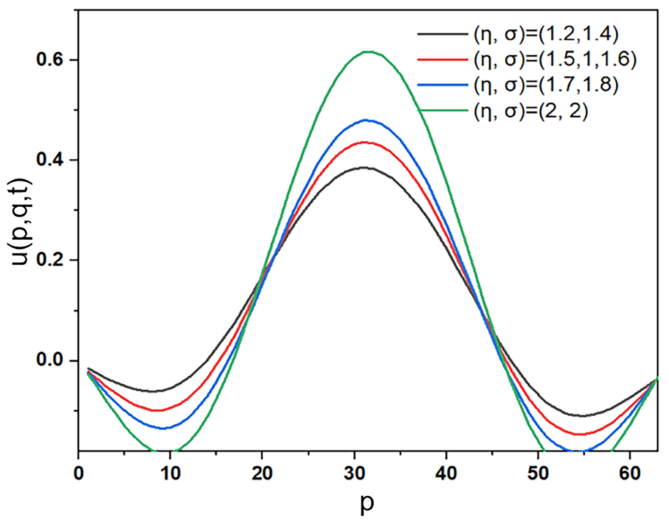
We solve the current problem using the proposed numerical method (27).

Table 1. Maximum errors, $L^2$ errors, convergence orders, and CPU time in seconds for Example 1 at $T=1,a_{\mathrm{p}}=a_{\mathrm{q}}=1,b_{\mathrm{p}}=b_{\mathrm{q}}=1.5$ with $\tau =h_{\mathrm{p}}=h_{\mathrm{q}}$.

$(\mathit{\eta },\mathit{\sigma })$	$\mathit{\tau }={\mathit{h}}_{\mathbf{p}}={\mathit{h}}_{\mathbf{q}}$	${\mathit{L}}^{\mathit{\infty }}-\mathbf{error}$	order${}_{\mathit{m}}$	${\mathit{L}}^2-\mathbf{error}$	order${}_2$	CPU(s)
(1.2, 1.8)	1/4	$1.8152\times {10}^{-6}$	-	$8.3261\times {10}^{-7}$	-	0.0020
	1/8	$5.2265\times {10}^{-7}$	1.7962	$2.2334\times {10}^{-7}$	1.8984	0.0059
	1/16	$1.4877\times {10}^{-7}$	1.8128	$5.5676\times {10}^{-8}$	2.0041	0.0288
	1/32	$3.6949\times {10}^{-8}$	2.0094	$1.3771\times {10}^{-8}$	2.0154	0.1724
	1/64	$9.2722\times {10}^{-9}$	1.9945	$3.4245\times {10}^{-9}$	2.0077	0.8077
	1/128	$2.316\times {10}^{-9}$	2.0013	$8.5576\times {10}^{-10}$	2.0006	5.8330
(1.3, 1.7)	1/4	$1.8533\times {10}^{-6}$	-	$8.1189\times {10}^{-7}$	-	0.0022
	1/8	$5.4362\times {10}^{-7}$	1.7694	$2.2393\times {10}^{-7}$	1.8583	0.0100
	1/16	$1.5247\times {10}^{-7}$	1.834	$5.7281\times {10}^{-8}$	1.9669	0.0837
	1/32	$3.8912\times {10}^{-8}$	1.9703	$1.447\times {10}^{-8}$	1.985	0.1850
	1/64	$9.8603\times {10}^{-9}$	1.9805	$3.6419\times {10}^{-9}$	1.9903	1.0993
	1/128	$2.4738\times {10}^{-9}$	1.9949	$9.1477\times {10}^{-10}$	1.9932	8.0243
(1.4, 1.6)	1/4	$1.8759\times {10}^{-6}$	-	$7.9874\times {10}^{-7}$	-	0.0020
	1/8	$5.5635\times {10}^{-7}$	1.7535	$2.2431\times {10}^{-7}$	1.8322	0.0066
	1/16	$1.531\times {10}^{-7}$	1.8615	$5.8323\times {10}^{-8}$	1.9434	0.0355
	1/32	$4.0374\times {10}^{-8}$	1.923	$1.4919\times {10}^{-8}$	1.9669	0.1485
	1/64	$1.023\times {10}^{-8}$	1.9806	$3.7801\times {10}^{-9}$	1.9806	0.8680
	1/128	$2.5736\times {10}^{-9}$	1.991	$9.5229\times {10}^{-10}$	1.989	6.9709

presents the maximum norm, $L^2$ norm errors, corresponding convergence orders, and computational time in seconds, obtained when $T=1,a_{\mathrm{p}}=a_{\mathrm{q}}=1,b_{\mathrm{p}}=b_{\mathrm{q}}=1.5$ with $\tau =h_{\mathrm{p}}=h_{\mathrm{q}}$ for $(\eta ,\sigma )=(1.2,1.8),(\eta ,\sigma )=(1.3,1.7),(\eta ,\sigma )=(1.4,1.6)$, respectively. In

Table 2. Results of CN-ADI and CN-non-ADI schemes for Example 1.

		CN–ADI			CN–non–ADI
$(\mathbf{\eta },\mathbf{\sigma })$	$\mathbf{\tau }={\mathit{h}}_{\mathrm{p}}={\mathit{h}}_{\mathrm{q}}$	${\mathit{l}}_{\infty }$	Order	CPU	${\mathit{l}}_{\infty }$	Order	CPU
	1/40	$2.3767\times {10}^{-8}$	-	0.1268	$2.3767\times {10}^{-8}$	-	0.2446
	1/80	$5.9314\times {10}^{-9}$	2.0025	0.7686	$5.9314\times {10}^{-9}$	2.0025	1.3055
(1.2,1.8)	1/160	$1.4824\times {10}^{-9}$	2.0004	5.9595	$1.4824\times {10}^{-9}$	2.0004	9.8197
	1/320	$3.7076\times {10}^{-10}$	1.9994	61.1540	$3.7076\times {10}^{-10}$	1.9994	72.0935
	1/40	$2.5151\times {10}^{-8}$	-	0.1395	$2.5151\times {10}^{-8}$	-	0.2249
	1/80	$6.3143\times {10}^{-9}$	1.9939	1.1048	$6.3143\times {10}^{-9}$	1.9939	1.4776
(1.3,1.7)	1/160	$1.584e\times {10}^{-9}$	1.995	7.7145	$1.584\times {10}^{-9}$	1.995	11.2881
	1/320	$3.9662\times {10}^{-10}$	1.9978	62.0667	$3.9662\times {10}^{-10}$	1.9978	82.0642
	1/40	$2.5961\times {10}^{-8}$	-	0.1492	$2.5961\times {10}^{-8}$	-	0.2446
	1/80	$6.5675\times {10}^{-9}$	1.9829	1.0746	$6.5675\times {10}^{-9}$	1.9829	1.3055
(1.4,1.6)	1/160	$1.649\times {10}^{-9}$	1.9938	7.7024	$1.649\times {10}^{-9}$	1.9938	9.8197
	1/320	$4.1311\times {10}^{-10}$	1.997	61.3860	$4.1311\times {10}^{-10}$	1.997	72.0935

, we examine the accuracy and computational processing unit (CPU) efficiency of the CN–ADI and CN–non–ADI schemes. We find that the accuracy of both methods is comparable, while the computational cost of the CN–ADI is lower than the computational cost of the CN–non–ADI scheme defined in (13). These results show that the CN–ADI scheme is more efficient. The error curves of Equation (28) for different values of $\eta ,\sigma$ and different grid points are displayed in Figure 1. In Figure 2, we present the behavior of the 2DNRSFCDE for different values of $\eta ,\sigma$ at $T=1$ with fixed $\tau =h_{\mathrm{p}}=h_{\mathrm{q}}=1/64$ and the diffusion coefficients $b_{\mathrm{p}}=b_{\mathrm{q}}=1.5$ and the convection coefficients $a_{\mathrm{p}}=a_{\mathrm{q}}=1$. It can be observed that our discretized scheme is second-order convergent in both time and space.

Example 2. 

Consider the 2DNRSFCDE below [32]:

$$\left\{\begin{array}{c}\frac{\partial \mathrm{u}(\mathrm{p},\mathrm{q},\mathrm{t})}{\partial \mathrm{t}}=-a_{\mathrm{p}}\frac{\partial \mathrm{u}(\mathrm{p},\mathrm{q},\mathrm{t})}{\partial \mathrm{p}}-a_{\mathrm{q}}\frac{\partial \mathrm{u}(\mathrm{p},\mathrm{q},\mathrm{t})}{\partial \mathrm{q}}+b_{\mathrm{p}}\frac{{\partial }^{\eta }\mathrm{u}(\mathrm{p},\mathrm{q},\mathrm{t})}{{\partial \left|\mathrm{p}\right|}^{\eta }}+b_{\mathrm{q}}\frac{{\partial }^{\sigma }\mathrm{u}(\mathrm{p},\mathrm{q},\mathrm{t})}{{\partial \left|\mathrm{q}\right|}^{\sigma }}-\mathrm{u}+f(\mathrm{p},\mathrm{q},\mathrm{t}),\hfill \\ \mathrm{u}(\mathrm{p},\mathrm{q},0)={\mathrm{p}}^2{(1-\mathrm{p})}^2{\mathrm{q}}^2{(1-\mathrm{q})}^2,0\le \mathrm{p},\mathrm{q}\le 1,\hfill \\ \mathrm{u}(0,\mathrm{q},\mathrm{t})=\mathrm{u}(1,\mathrm{q},\mathrm{t})=\mathrm{u}(\mathrm{p},0,\mathrm{t})=\mathrm{u}(\mathrm{p},1,\mathrm{t})=0,0\le \mathrm{p},\mathrm{q}\le 1,0<\mathrm{t}\le T,\hfill \end{array}\right.$$

(29)

where

$$\begin{array}{ccc}\hfill f(\mathrm{p},\mathrm{q},\mathrm{t})& =& e^{-\mathrm{t}}{\mathrm{p}}^2{(1-\mathrm{p})}^2{\mathrm{q}}^2{(1-\mathrm{q})}^2+a_{\mathrm{p}}{e}^{-\mathrm{t}}(2\mathrm{p}{(\mathrm{p}-1)}^2+{\mathrm{p}}^2(2\mathrm{p}-2){\mathrm{q}}^2{(1-\mathrm{q})}^2)\hfill \\ & +& a_{\mathrm{q}}{e}^{-\mathrm{t}}(2\mathrm{q}{(\mathrm{q}-1)}^2+{\mathrm{q}}^2(2\mathrm{q}-2){\mathrm{p}}^2{(1-\mathrm{p})}^2)\hfill \\ & -& b_{\mathrm{p}}{\kappa }_{\eta }{e}^{-\mathrm{t}}{\mathrm{q}}^2{(1-\mathrm{q})}^2[\frac{2}{\mathsf{\Gamma }(3-\eta )}\left({\mathrm{p}}^{2-\eta }+{(1-\mathrm{p})}^{2-\eta }\right)-\frac{12}{\mathsf{\Gamma }(4-\eta )}\left({\mathrm{p}}^{3-\eta }+{(1-\mathrm{p})}^{3-\eta }\right)\hfill \\ & +& \frac{24}{\mathsf{\Gamma }(5-\eta )}\left({\mathrm{p}}^{4-\eta }+{(1-\mathrm{p})}^{4-\eta }\right)]\hfill \\ & -& b_{\mathrm{q}}{\kappa }_{\sigma }{e}^{-\mathrm{t}}{\mathrm{p}}^2{(1-\mathrm{p})}^2[\frac{2}{\mathsf{\Gamma }(3-\sigma )}\left({\mathrm{q}}^{2-\sigma }+{(1-\mathrm{q})}^{2-\sigma }\right)-\frac{12}{\mathsf{\Gamma }(4-\sigma )}\left({\mathrm{q}}^{3-\sigma }+{(1-\mathrm{q})}^{3-\sigma }\right)\hfill \\ & +& \frac{24}{\mathsf{\Gamma }(5-\sigma )}\left({\mathrm{q}}^{4-\sigma }+{(1-\mathrm{q})}^{4-\sigma }\right)].\hfill \end{array}$$

The exact solution for Equation (29) is $\mathrm{u}(\mathrm{p},\mathrm{q},\mathrm{t})=e^{-\mathrm{t}}{\mathrm{p}}^2{(1-\mathrm{p})}^2{\mathrm{q}}^2{(1-\mathrm{q})}^2$. In

Table 3. Maximum errors, $L^2$ errors, convergence orders, and CPU time in seconds for Example 2 at $T=1,a_{\mathrm{p}}=a_{\mathrm{q}}=1,b_{\mathrm{p}}=b_{\mathrm{q}}=1.2$ with $\tau =h_{\mathrm{p}}=h_{\mathrm{q}}$.

$(\mathit{\eta },\mathit{\sigma })$	$\mathit{\tau }={\mathit{h}}_{\mathbf{p}}={\mathit{h}}_{\mathbf{q}}$	${\mathit{L}}^{\mathit{\infty }}-\mathit{error}$	order${}_{\mathit{m}}$	${\mathit{L}}^2-\mathit{error}$	order${}_2$	CPU(s)
(1.2, 1.8)	1/4	$2.1441\times {10}^{-3}$	-	$9.9306\times {10}^{-4}$	-	0.0164
	1/8	$5.1681\times {10}^{-4}$	2.0527	$2.4656\times {10}^{-4}$	2.0099	0.0076
	1/16	$1.2652\times {10}^{-4}$	2.0303	$6.0392\times {10}^{-5}$	2.0295	0.0155
	1/32	$3.0962\times {10}^{-5}$	2.0308	$1.4653\times {10}^{-5}$	2.0431	0.1361
	1/64	$7.5627\times {10}^{-6}$	2.0335	$3.5437\times {10}^{-6}$	2.0479	0.6257
	1/128	$2.1095\times {10}^{-6}$	1.842	$8.5769\times {10}^{-7}$	2.0467	3.8980
(1.3, 1.7)	1/4	$2.2092\times {10}^{-3}$	-	$9.9462\times {10}^{-4}$	-	0.0077
	1/8	$5.3103\times {10}^{-4}$	2.0566	$2.4417\times {10}^{-4}$	2.0263	0.0077
	1/16	$1.2932\times {10}^{-4}$	2.0378	$5.9397\times {10}^{-5}$	2.0394	0.0336
	1/32	$3.1383\times {10}^{-5}$	2.0429	$1.4402\times {10}^{-5}$	2.0442	0.1148
	1/64	$8.3628\times {10}^{-6}$	1.9079	$3.5005\times {10}^{-6}$	2.0406	0.5898
	1/128	$2.5474\times {10}^{-6}$	1.715	$8.5536\times {10}^{-7}$	2.033	3.9085
(1.4, 1.6)	1/4	$2.2463\times {10}^{-3}$	-	$9.9341\times {10}^{-4}$	-	0.0038
	1/8	$5.3872\times {10}^{-4}$	2.0599	$2.4241\times {10}^{-4}$	2.0349	0.0084
	1/16	$1.3074\times {10}^{-4}$	2.0428	$5.8792\times {10}^{-5}$	2.0438	0.0367
	1/32	$3.1552\times {10}^{-5}$	2.0509	$1.4277\times {10}^{-5}$	2.0419	0.1276
	1/64	$7.9727\times {10}^{-6}$	1.9846	$3.4954e\times {10}^{-6}$	2.0302	0.5947
	1/128	$2.4315\times {10}^{-6}$	1.7132	$8.6459\times {10}^{-7}$	2.0154	3.9343

, we display the maximum, $L^2$ errors with their related estimated convergence orders, and the computational time at $T=1,a_{\mathrm{p}}=a_{\mathrm{q}}=1,b_{\mathrm{p}}=b_{\mathrm{q}}=1.2$ with $\tau =h_{\mathrm{p}}=h_{\mathrm{q}}$.

The error curves of Equation (29) for different values of $\eta ,\sigma$ and different step sizes are illustrated in Figure 3. In Figure 4, we present the behavior of the 2DNRSFCDE for different values of $\eta ,\sigma$ at $T=1$ with fixed $\tau =h_{\mathrm{p}}=h_{\mathrm{q}}=1/64$ and the diffusion coefficients $b_{\mathrm{p}}=b_{\mathrm{q}}=1.2$ and the convection coefficients $a_{\mathrm{p}}=a_{\mathrm{q}}=1$. We see that the method yields $\mathcal{O}({\tau }^2+h_{\mathrm{p}}^2+h_{\mathrm{q}}^2)$ convergence, as expected. It shows that our proposed difference scheme is accurate and effective. In

Table 4. Maximum errors, convergence orders for Example 2 at $T=1,b_{\mathrm{p}}=b_{\mathrm{q}}=0.5$ with $\tau =h_{\mathrm{p}}=h_{\mathrm{q}}$.

		Scheme (27)		[32]
$(\mathbf{\eta },\mathbf{\sigma })$	$\mathbf{\tau }={\mathit{h}}_{\mathrm{p}}={\mathit{h}}_{\mathrm{q}}$	${\mathit{l}}_{\infty }$	Order	${\mathit{l}}_{\infty }$	Order
	1/40	$5.5484\times {10}^{-6}$	-	$5.6949\times {10}^{-5}$	-
	1/80	$1.3355\times {10}^{-6}$	2.0547	$2.9406\times {10}^{-5}$	0.9536
(1.5,1.5)	1/160	$3.22\times {10}^{-7}$	2.0522	$1.4925\times {10}^{-5}$	0.9703
	1/320	$7.7859\times {10}^{-8}$	2.0481	$7.5139\times {10}^{-6}$	0.9901

, we give the comparison of the maximum error and convergence order of our scheme (27) with the results in [32] at $(\eta ,\sigma )=(1.5,1.5)$, $T=1,a_{\mathrm{p}}=a_{\mathrm{q}}=0,b_{\mathrm{p}}=b_{\mathrm{q}}=0.5$ with $\tau =h_{\mathrm{p}}=h_{\mathrm{q}}$. The maximum error presented in the scheme (27) is more accurate than the maximum error obtained in [32]. We obtain second–order convergence in our proposed scheme while the convergence order in [32] is linear.

6. Conclusions

In this paper, the Crank–Nicolson method in the time direction and the weighted–shifted Grünwald–Letnikov difference method in space discretization are proposed to formulate and analyze the nonlinear Riesz space–fractional convection–diffusion equation in two dimensions on a finite domain. To find the solution of the two–dimensional problem alternatively and obtain the reduced one-dimensional problem with an efficient computational cost, we used the D’Yakonov ADI approach. Moreover, we have investigated the unconditional stability and convergence of the formulated problem, which illustrates the CNADI–WSGD scheme with $\mathcal{O}({\tau }^2+h_{\mathrm{p}}^2+h_{\mathrm{q}}^2)$ accuracy. We have performed numerical simulations to justify the validity of our theoretical analysis results, which are in good agreement with the theoretical results. Because solving nonlinear space-fractional problems is one of the most difficult challenges, the existing approaches are rarely constructed to solve the problems. Most of the existing studies focused on the linear space-fractional equations, see [22,23,26,27,30,31,40]. The CNADI–WSGD discretization defined by (27) has second-order temporal and spatial accuracy, while the numerical schemes implemented in [32,45] have first-order accuracy in both the temporal and spatial directions. As we have seen in Table 1 and Table 3, when we refine the grid point in both the time and space directions, the $L_{\infty }$ error and $L_2$ error are also decreased and obtain second–order accuracy. As the comparison result is shown in Table 4, our scheme gives second-order convergence, which implies that our constructed scheme is more precise and effective. A highly recommended line of study for future research is to extend this method to solve other fractional differential equations.

References

- Miller, K.S.; Ross, B. An Introduction to the Fractional Calculus and Fractional Differential Equations; John Wiley & Sons Inc.: New York, NY, USA, 1993. [Google Scholar]
- Hilfer, R. Applications of Fractional Calculus in Physics; World Scientific: Singapore, 2000. [Google Scholar]
- Sheng, H.; Chen, Y.; Qiu, T. Fractional Processes and Fractional-Order Signal Processing: Techniques and Applications; Springer: London, UK, 2011. [Google Scholar]
- Fomin, S.; Chugunov, V.; Hashida, T. Application of fractional differential equations for modeling the anomalous diffusion of contaminant from fracture into porous rock matrix with bordering alteration zone. Transp. Porous Media 2010, 2, 187–205. [Google Scholar] [CrossRef]
- Wang, K.; Wang, H. A fast characteristic finite difference method for fractional advection–diffusion equations. Adv. Water Resour. 2011, 7, 810–816. [Google Scholar] [CrossRef]
- Magin, R.L. Fractional calculus models of complex dynamics in biological tissues. Comput. Math. Appl. 2010, 5, 1586–1593. [Google Scholar] [CrossRef] [Green Version]
- Sabatelli, L.; Keating, S.; Dudley, J.; Richmond, P. Waiting time distributions in financial markets. Eur. Phys. J. B 2002, 2, 273–275. [Google Scholar] [CrossRef]
- Basha, M.; Dai, B.; Al-Sadi, W. Existence and stability for a nonlinear coupled p-laplacian system of fractional differential equations. J. Math. 2021, 2021, 6687949. [Google Scholar] [CrossRef]
- Hejazi, H.; Moroney, T.; Liu, F. Stability and convergence of a finite volume method for the space fractional advection–dispersion equation. Comput. Appl. Math. 2014, 255, 684–697. [Google Scholar] [CrossRef] [Green Version]
- Jia, J.; Wang, H. A fast finite volume method for conservative space-fractional diffusion equations in convex domains. J. Comput. Phys. 2016, 310, 63–84. [Google Scholar] [CrossRef] [Green Version]
- Jin, B.; Lazarov, R.; Zhou, Z. A Petrov–Galerkin finite element method for fractional convection-diffusion equations. SIAM J. Numer. Anal. 2016, 1, 481–503. [Google Scholar] [CrossRef] [Green Version]
- Fu, T.; Duan, B.; Zheng, Z. An Effective Finite Element Method with Singularity Reconstruction for Fractional Convection-diffusion Equation. J. Sci. Comput. 2021, 3, 1–18. [Google Scholar] [CrossRef]
- Shen, J.; Stynes, M.; Sun, Z.Z. Two Finite Difference Schemes for Multi-Dimensional Fractional Wave Equations with Weakly Singular Solutions. Comput. Methods Appl. Math. 2021, 4, 913–928. [Google Scholar] [CrossRef]
- Li, C.; Zeng, F. Finite difference methods for fractional differential equations. Int. J. Bifurc. Chaos Appl. Sci. Eng. 2012, 4, 1230014. [Google Scholar] [CrossRef]
- Anley, E.F.; Zheng, Z. Finite difference approximation method for a space fractional convection–diffusion equation with variable coefficients. Symmetry 2020, 3, 485. [Google Scholar] [CrossRef] [Green Version]
- Huang, J.F.; Nie, N.; Tang, Y. Second order finite difference-spectral method for space fractional diffusion equations. Sci. China Math. 2014, 6, 1303–1317. [Google Scholar] [CrossRef]
- Basha, M.; Anley, E.F.; Dai, B. Numerical Solution for a Nonlinear Time-Space Fractional Convection-Diffusion Equation. J. Comput. Nonlinear Dyn. 2022, 1, 1–22. [Google Scholar] [CrossRef]
- Doha, E.H.; Bhrawy, A.H.; Baleanu, D.; Ezz-Eldien, S.S. On shifted Jacobi spectral approximations for solving fractional differential equations. Appl. Math. Comput. 2013, 15, 8042–8056. [Google Scholar] [CrossRef]
- Behroozifar, M.; Ahmadpour, F. A study on spectral methods for linear and nonlinear fractional differential equations. Int. J. Comput. Sci. Math. 2019, 6, 545–556. [Google Scholar] [CrossRef]
- Xu, Q.; Hesthaven, J.S. Discontinuous Galerkin method for fractional convection-diffusion equations. SIAM J. Numer. Anal. 2014, 1, 405–423. [Google Scholar] [CrossRef] [Green Version]
- Mustapha, K. Time-stepping discontinuous Galerkin methods for fractional diffusion problems. Numer. Math. 2015, 3, 497–516. [Google Scholar] [CrossRef] [Green Version]
- Feng, L.B.; Zhuang, P.; Liu, F.; Turner, I.; Li, J. High-order numerical methods for the Riesz space fractional advection-dispersion equations. Comput. Math. Appl. 2016. [Google Scholar] [CrossRef]
- Tian, W.; Deng, W.; Wu, Y. Polynomial spectral collocation method for space fractional advection–diffusion equation. Numer. Methods Partial Differ. Equ. 2015, 2, 514–535. [Google Scholar] [CrossRef] [Green Version]
- Bhrawy, A.H.; Baleanu, D. A spectral Legendre–Gauss–Lobatto collocation method for a space-fractional advection diffusion equations with variable coefficients. Rep. Math. Phys. 2013, 2, 219–233. [Google Scholar] [CrossRef]
- Xie, J.; Huang, Q.; Yang, X. Numerical solution of the one-dimensional fractional convection diffusion equations based on Chebyshev operational matrix. SpringerPlus 2016, 5, 1149. [Google Scholar] [CrossRef] [PubMed] [Green Version]
- Borhanifar, A.; Ragusa, M.A.; Valizadehaz, S. High-order numerical method for two-dimensional Riesz space fractional advection-dispersion equation. Discrete Contin. Dyn. Syst. Ser. B 2020, 10, 5495–5508. [Google Scholar]
- Chen, M.; Deng, W. A second-order numerical method for two-dimensional two-sided space fractional convection diffusion equation. Appl. Math. Model. 2014, 13, 3244–3259. [Google Scholar] [CrossRef]
- Chen, M.; Deng, W. Fourth order accurate scheme for the space fractional diffusion equations. SIAM J. Numer. Anal. 2014, 3, 1418–1438. [Google Scholar] [CrossRef] [Green Version]
- Hou, D.; Azaiez, M.; Xu, C. Müntz Spectral Method for Two-Dimensional Space-Fractional Convection-Diffusion Equation. Commun. Comput. Phys. 2019, 26, 1415–1443. [Google Scholar] [CrossRef]
- Zhou, Y.; Zhang, C.; Brugnano, L. An implicit difference scheme with the KPS preconditioner for two-dimensional time–space fractional convection–diffusion equations. Comput. Math. Appl. 2020, 1, 31–42. [Google Scholar] [CrossRef]
- Bi, Y.; Jiang, Z. The finite volume element method for the two-dimensional space-fractional convection–diffusion equation. Adv. Differ. Equ. 2021, 2021, 379. [Google Scholar] [CrossRef]
- Liu, F.; Chen, S.; Turner, I.; Burrage, K.; Anh, V. Numerical simulation for two-dimensional Riesz space fractional diffusion equations with a nonlinear reaction term. Cent. Eur. J. Phys. 2013, 10, 1221–1232. [Google Scholar] [CrossRef] [Green Version]
- Zeng, F.; Liu, F.; Li, C.; Burrage, K.; Turner, I.; Anh, V. A Crank–Nicolson ADI spectral method for a two-dimensional Riesz space fractional nonlinear reaction-diffusion equation. SIAM J. Numer. Anal. 2014, 6, 2599–2622. [Google Scholar] [CrossRef] [Green Version]
- Zhu, X.; Nie, Y.; Wang, J.; Yuan, Z. A numerical approach for the Riesz space-fractional Fisher’equation in two-dimensions. Int. J. Comput. Math. 2017, 2, 296–315. [Google Scholar] [CrossRef]
- Yang, S. Numerical simulation for the two-dimensional and three-dimensional Riesz space fractional diffusion equations with delay and a nonlinear reaction term. Int. J. Comput. Math. 2019, 10, 1957–1978. [Google Scholar] [CrossRef]
- Samko, S.G.; Kilbas, A.A.; Marichev, O.I. Fractional Integrals and Derivatives: Theory and Applications; Gordon and Breach Science Publishers: Yverdon-les-Bains, Switzerland, 1993. [Google Scholar]
- Kilbas, A.A.A.; Srivastava, H.M.; Trujillo, J.J. Theory and Applications of Fractional Differential Equations; Elsevier Science Limited: Amsterdam, The Netherlands, 2006. [Google Scholar]
- Podlubny, I. Fractional Differential Equations; Academic Press: San Diego, CA, USA, 1999. [Google Scholar]
- Liu, F.; Anh, V.; Turner, I. Numerical solution of the space fractional Fokker–Planck equation. J. Comput. Appl. Math. 2004, 1, 209–219. [Google Scholar] [CrossRef] [Green Version]
- Anley, E.F.; Zheng, Z. Finite Difference Method for Two-Sided Two Dimensional Space Fractional Convection-Diffusion Problem with Source Term. Mathematics 2020, 11, 1878. [Google Scholar] [CrossRef]
- Tian, W.; Zhou, H.; Deng, W. A class of second order difference approximations for solving space fractional diffusion equations. Math. Comput. 2015, 294, 1703–1727. [Google Scholar] [CrossRef] [Green Version]
- Meerschaert, M.M.; Tadjeran, C. Finite difference approximations for two-sided space-fractional partial differential equations. Appl. Numer. Math. 2006, 1, 80–90. [Google Scholar] [CrossRef]
- Thomas, J.W. Numerical Partial Differential Equations: Finite Difference Methods; Springer Science & Business Media: Berlin/Heidelberg, Germany, 2013. [Google Scholar]
- Yu, D.; Tan, H. Numerical Methods of Differential Equations; Science Publisher: Beijing, China, 2003. [Google Scholar]
- Nasrollahzadeh, F.; Hosseini, S.M. An implicit difference-ADI method for the two-dimensional space-time fractional diffusion equation. Iran. J. Math. Sci. Inform. 2016, 2, 71–86. [Google Scholar]
Figure 1.
Errors of the computed scheme of Example 1 with for different and grid points: (a) , (b) .
Figure 2.
The numerical solution of for the 2DNRSFCDE (28) at with different when .
Figure 3.
Errors of the computed scheme of Example (2) with for different and grid points: (a) , (b) .
Figure 4.
The numerical approximation of for the 2DNRSFCDE (29) at with different when .