Novel Fractional Models Compatible with Real World Problems

Abstract

In this paper, some real world modeling problems: vertical motion of a falling body problem in a resistant medium, and the Malthusian growth equation, are considered by the newly defined Liouville–Caputo fractional conformable derivative and the modified form of this new definition. We utilize the $\sigma$ auxiliary parameter for preserving the dimension of physical quantities for newly defined fractional conformable vertical motion of a falling body problem in a resistant medium. The analytical solutions are obtained by iterating this new fractional integral and results are illustrated under different orders by comparison with the Liouville–Caputo fractional operator.

1. Introduction

Fractional differential equations were first suggested as an idea by Leibniz on generalizing the integer order derivative about three centuries ago. From this point of view, they introduced Riemann–Liouville and Liouville–Caputo fractional derivatives. Very recently, Jarad et al. [1] have introduced a new fractional derivative called the Liouville-Caputo fractional conformable derivative. Nowadays, fractional derivatives have been begun to be applied to real world modeling problems [2,3,4,5,6,7,8]. However, many new fractional derivative definitions have been introduced in recent years. Some of those are Atangana–Baleanu [9], Hilfer [10], Hadamard [11], Caputo–Fabrizio [12], etc. The Liouville-Caputo fractional conformable derivative is a fractional form of conformable derivative introduced by Abdeljawad [13]. On the other hand, Delgado et al. [2] used this new fractional definition for electrical circuits and they made contribution to this new definition by introducing the $\beta$-form of this new fractional definition. The $\beta$-form of conformable derivative has been introduced by Atangana [14]. However, the conformable derivative idea has been firstly suggested by Khalil et al. [15] and thereafter a different form of this definition called as proportional $\alpha$-derivative has been defined in [16]. On the other hand, you can find new studies about this new generalized fractional conformable definition in [17,18,19,20]. Some studies about fractional differential equations and its applications are studied in [21,22,23,24,25].

In this paper, we consider firstly the vertical motion of a falling body problem in a resistant medium and it is defined as in the classical meaning as

$$m\frac{dv\left(t\right)}{dt}=-mg-mkv\left(t\right),$$

$$v\left(0\right)=v_0,$$

where $v\left(t\right)$ (m/s) is velocity, t (s) is time, g (m/s${}^2$) is a gravitational force, m (kg) is mass, and k (s${}^{-1}$) air drag. If we fractionalize the ordinary derivative, we must make use of the $\sigma$ auxiliary parameter, which has $tim{e}^{-1}$ ( s${}^{-1}$) dimension, for preserving the dimension of physical quantities, so we get

$$\frac{d}{dt}\to {\sigma }^{1-\alpha \beta }{}_a^{C\beta }{D}_t^{\alpha }$$

where ${}_a^{C\beta }{D}_t^{\alpha }$ is Liouville-Caputo fractional conformable derivative operator introduced by Jarad et al. [1]. We consider a similar case with beta form of Liouville-Caputo fractional conformable derivative defined by Delgado et al. [2]. This approach will shed a light on future studies including fractional physical problems.

In population biology, we use the Malthusian growth model to define animal population or the growth of tumor and bacteria. Fractional models of these equations give more sensitive results than the integer order differential equations. The Malthusian growth model is used to guess approximately in the change of the population in time. It is also used to guess the approximate numbers of bacterial culture, approximate radioactive decay time, etc., and it is defined classically as

$$P^{\prime }\left(t\right)=kP\left(t\right),$$

where $P\left(t\right)$ is the population, k is the change rate.

2. Preliminaries

Definition 1.

[21] The Riemann-Liouville derivative of order α is defined as

$${}_a^{RL}{D}_x^{\alpha }f\left(x\right)=\frac{1}{\mathsf{\Gamma }\left(n-\alpha \right)}\frac{d^n}{d{t}^n}\underset{a}{\overset{x}{\int }}f\left(t\right){\left(x-t\right)}^{n-\alpha -1}dt,n-1<\alpha <n.$$

Definition 2.

[21] The Liouville–Caputo derivative definition of order α is defined as

$${}_a^C{D}_x^{\alpha }f\left(t\right)=\frac{1}{\mathsf{\Gamma }\left(n-\alpha \right)}\underset{a}{\overset{x}{\int }}\frac{d^n}{d{t}^n}f\left(t\right){\left(x-t\right)}^{n-\alpha -1}dt,n-1<\alpha <n.$$

Definition 3.

[21] Let $z,$ $\beta \in \mathbb{C},Re\left(\alpha \right)>0$. Then Mittag–Leffler function with two parameters is defined as

$$E_{\alpha ,\beta }\left(z\right)=\sum _{k=0}^{\infty }\frac{z^k}{\mathsf{\Gamma }\left(\alpha k+\beta \right)}.$$

Definition 4.

[15] Let $f:\left[a,\infty \right)\to \mathbb{R}.$ The conformable derivative of $f\left(t\right)$ is defined as follows

$$D_t^{\alpha }f\left(t\right)=\underset{\epsilon \to 0}{lim}\frac{f\left(t+\epsilon t^{1-\alpha }\right)-f\left(t\right)}{\epsilon }$$

for all $t>0,$ $\alpha \in \left(0,1\right].$ If $f\left(t\right)$ is $\alpha -$ differentiable in some $\left(0,a\right),$ $a>0$ and if $\underset{\epsilon \to 0^{+}}{lim}{f}^{\left(\alpha \right)}\left(t\right)$ exists, then define $\underset{t\to 0^{+}}{lim}{f}^{\left(\alpha \right)}\left(t\right)=f^{\left(\alpha \right)}\left(0\right).$

Definition 5.

[13] Let $f:\left[a,\infty \right)\to \mathbb{R}.$ The left and right conformable derivative of $f\left(t\right)$ is defined as follows respectively

$$\begin{array}{c}\hfill {}_a{D}_t^{\alpha }f\left(t\right)=\underset{\epsilon \to 0}{lim}\frac{f\left(t+\epsilon {(t-a)}^{1-\alpha }\right)-f\left(t\right)}{\epsilon },\\ \hfill {}_t{D}_b^{\alpha }f\left(t\right)=\underset{\epsilon \to 0}{lim}\frac{f\left(t+\epsilon {(b-t)}^{1-\alpha }\right)-f\left(t\right)}{\epsilon },\end{array}$$

for all $t>0,$ $\alpha \in \left(0,1\right].$

Definition 6.

[13,15] The left and right conformable integrals are defined as

$${}_a{I}^{\alpha }f\left(x\right)=\underset{a}{\overset{x}{\int }}{\left(t-a\right)}^{\alpha -1}f\left(t\right)dt,x\ge a,0<\alpha \le 1$$

(1)

$$I_b^{\alpha }f\left(x\right)=\underset{x}{\overset{b}{\int }}{\left(b-t\right)}^{\alpha -1}f\left(t\right)dt,x\le b.$$

Definition 7.

[1] Fractional conformable integral is defined as, $\beta \in \mathbb{R},Re\left(\beta \right)>0,$

$${}_a^{\beta }{I}^{\alpha }f\left(x\right)=\frac{1}{\mathsf{\Gamma }\left(\beta \right)}\underset{a}{\overset{x}{\int }}{\left(\frac{{\left(x-a\right)}^{\alpha }-{\left(t-a\right)}^{\alpha }}{\alpha }\right)}^{\beta -1}\frac{f\left(t\right)}{{\left(t-a\right)}^{1-\alpha }}dt.$$

(2)

Theorem 1.

[1] Let $Re\left(\beta \right)\ge 0,$ $n=\left[Re\left(\beta \right)\right]+1,$ $f\in C_{\alpha ,a}^n\left(\left[a,b\right]\right).$ Then, Riemann-Liouville fractional conformable derivatives are defined as follows,

$${}_a^{\beta }{D}^{\alpha }f\left(x\right)=\frac{{}_a^n{D}^{\alpha }f\left(t\right)}{\mathsf{\Gamma }\left(n-\beta \right)}\underset{a}{\overset{x}{\int }}{\left(\frac{{\left(x-a\right)}^{\alpha }-{\left(t-a\right)}^{\alpha }}{\alpha }\right)}^{n-\beta -1}\frac{f\left(t\right)}{{\left(t-a\right)}^{1-\alpha }}dt,$$

(3)

and

$${}^{\beta }{D}_b^{\alpha }f\left(x\right)=\frac{{\left(-1\right)}^n{}^n{D}_b^{\alpha }f\left(t\right)}{\mathsf{\Gamma }\left(n-\beta \right)}\underset{x}{\overset{b}{\int }}{\left(\frac{{\left(b-x\right)}^{\alpha }-{\left(b-t\right)}^{\alpha }}{\alpha }\right)}^{n-\beta -1}\frac{f\left(t\right)}{{\left(b-t\right)}^{1-\alpha }}dt,$$

(4)

where ${}_a^n{D}^{\alpha }$ and ${}^n{D}_b^{\alpha }$ are the left and right conformable derivatives.

Proof. 

You can find the proof of this theorem in [1]. □

Theorem 2.

[1] Let $Re\left(\beta \right)\ge 0,$ $n=\left[Re\left(\beta \right)\right]+1,$ $f\in C_{\alpha ,a}^n\left(\left[a,b\right]\right).$ Then, Liouville–Caputo fractional conformable derivatives are given by,

$${}_a^{C\beta }{D}^{\alpha }f\left(x\right)=\frac{1}{\mathsf{\Gamma }\left(n-\beta \right)}\underset{a}{\overset{x}{\int }}{\left(\frac{{\left(x-a\right)}^{\alpha }-{\left(t-a\right)}^{\alpha }}{\alpha }\right)}^{n-\beta -1}\frac{{}_a^n{D}^{\alpha }f\left(t\right)}{{\left(t-a\right)}^{1-\alpha }}dt,$$

(5)

and

$${}^{C\beta }{D}_b^{\alpha }f\left(x\right)=\frac{{\left(-1\right)}^n}{\mathsf{\Gamma }\left(n-\beta \right)}\underset{x}{\overset{b}{\int }}{\left(\frac{{\left(b-x\right)}^{\alpha }-{\left(b-t\right)}^{\alpha }}{\alpha }\right)}^{n-\beta -1}\frac{{}^n{D}_b^{\alpha }f\left(t\right)}{{\left(b-t\right)}^{1-\alpha }}dt.$$

(6)

Proof. 

You can find the proof of this theorem in [1]. □

Definition 8.

[14] Let $f:\left[-\frac{a}{\mathsf{\Gamma }\left(\alpha \right)},\infty \right)\to \mathbb{R},$ then a different type of conformable derivative of $f\left(t\right)$ is defined as

$${}_0^A{D}^{\alpha }f\left(x\right)=\underset{\epsilon \to 0}{lim}\frac{f\left(t+\epsilon {\left(t+\frac{1}{\mathsf{\Gamma }\left(\alpha \right)}\right)}^{1-\alpha }\right)-f\left(t\right)}{\epsilon }.$$

The different type of left conformable integral is defined as

$${}_0^A{I}^{\alpha }f\left(x\right)=\underset{0}{\overset{t}{\int }}\frac{f\left(x\right)}{{\left(x+\frac{1}{\mathsf{\Gamma }\left(\alpha \right)}\right)}^{1-\alpha }},0<\alpha \le 1.$$

Theorem 3.

[2] Let $Re\left(\beta \right)\ge 0,$ $n=\left[Re\left(\beta \right)\right]+1,$ $f\in C_{\alpha ,a}^n\left(\left[a,b\right]\right).$ Then a different type of Liouville–Caputo fractional conformable derivatives are defined as follows,

$${}_a^{AC\beta }{D}^{\alpha }f\left(x\right)=\frac{1}{\mathsf{\Gamma }\left(n-\beta \right)}\underset{-\frac{a}{\mathsf{\Gamma }\left(\alpha \right)}}{\overset{x}{\int }}{\left(\frac{{\left(x+\frac{a}{\mathsf{\Gamma }\left(\alpha \right)}\right)}^{\alpha }-{\left(t+\frac{a}{\mathsf{\Gamma }\left(\alpha \right)}\right)}^{\alpha }}{\alpha }\right)}^{n-\beta -1}\frac{{}_a^{An}{D}_{t-}^{\alpha }f\left(t\right)}{{\left(t+\frac{a}{\mathsf{\Gamma }\left(\alpha \right)}\right)}^{1-\alpha }}dt,$$

(7)

and

$${}^{AC\beta }{D}_b^{\alpha }f\left(x\right)=\frac{{\left(-1\right)}^n}{\mathsf{\Gamma }\left(n-\beta \right)}\underset{x}{\overset{-\frac{b}{\mathsf{\Gamma }\left(\alpha \right)}}{\int }}{\left(\frac{{\left(\frac{b}{\mathsf{\Gamma }\left(\alpha \right)}+t\right)}^{\alpha }-{\left(\frac{b}{\mathsf{\Gamma }\left(\alpha \right)}+x\right)}^{\alpha }}{\alpha }\right)}^{n-\beta -1}\frac{{}_t^{An}{D}_{b-}^{\alpha }f\left(t\right)}{{\left(\frac{b}{\mathsf{\Gamma }\left(\alpha \right)}+t\right)}^{1-\alpha }}dt.$$

(8)

Proof. 

You can find the proof of this theorem in [2]. □

Theorem 4.

[2] Let $Re\left(\beta \right)\ge 0,$ $n=\left[Re\left(\beta \right)\right]+1,$ $f\in C_{\alpha ,a}^n\left(\left[a,b\right]\right).$ Then a different type of Riemann-Liouville fractional conformable derivatives are defined as follows,

$${}_a^{AR\beta }{D}^{\alpha }f\left(x\right)=\frac{{}_a^{An}{D}^{\alpha }}{\mathsf{\Gamma }\left(n-\beta \right)}\underset{a}{\overset{x}{\int }}{\left(\frac{{\left(x+\frac{a}{\mathsf{\Gamma }\left(\alpha \right)}\right)}^{\alpha }-{\left(t+\frac{a}{\mathsf{\Gamma }\left(\alpha \right)}\right)}^{\alpha }}{\alpha }\right)}^{n-\beta -1}\frac{f\left(t\right)}{{\left(t+\frac{a}{\mathsf{\Gamma }\left(\alpha \right)}\right)}^{1-\alpha }}dt,$$

(9)

and

$${}^{AR\beta }{D}_b^{\alpha }f\left(x\right)=\frac{{\left(-1\right)}_{}^{nAn}{D}_b^{\alpha }}{\mathsf{\Gamma }\left(n-\beta \right)}\underset{x}{\overset{b}{\int }}{\left(\frac{{\left(\frac{b}{\mathsf{\Gamma }\left(\alpha \right)}+t\right)}^{\alpha }-{\left(\frac{b}{\mathsf{\Gamma }\left(\alpha \right)}+x\right)}^{\alpha }}{\alpha }\right)}^{n-\beta -1}\frac{f\left(t\right)}{{\left(\frac{b}{\mathsf{\Gamma }\left(\alpha \right)}+t\right)}^{1-\alpha }}dt.$$

(10)

Proof. 

You can find the proof of this theorem in [2]. □

Theorem 5.

[2] Let $f\in C_{\alpha ,a}^n\left(\left[a,b\right]\right),$ $\beta \in \mathbb{R}.$ Then the following property is valid,

$${}_a^{\beta }{I}^{\alpha }\left({}_a^{AC\beta }{D}^{\alpha }f\left(t\right)\right)=f\left(t\right)-\sum _{k=0}^{n-1}\frac{{}_a^k{D}_t^{\alpha }f\left(a\right){\left(t-a\right)}^{\alpha k}}{{\alpha }^{k}k!},$$

and

$${}_a^{\beta }{I}^{\alpha }\left({}_a^{AC\beta }{D}^{\alpha }f\left(t\right)\right)=f\left(t\right)-\sum _{k=0}^{n-1}\frac{{\left(-1\right)}^k{}_t^k{D}_b^{\alpha }f\left(b\right){\left(b-t\right)}^{\alpha k}}{{\alpha }^{k}k!}.$$

Proof. 

You can find the proof of this theorem in [2]. □

3. Main Results

In this section, we find exact analytical solutions of vertical motion of falling body problem in the resistant medium, and fractional Malthusian growth model with newly defined Liouville-Caputo fractional conformable derivative.

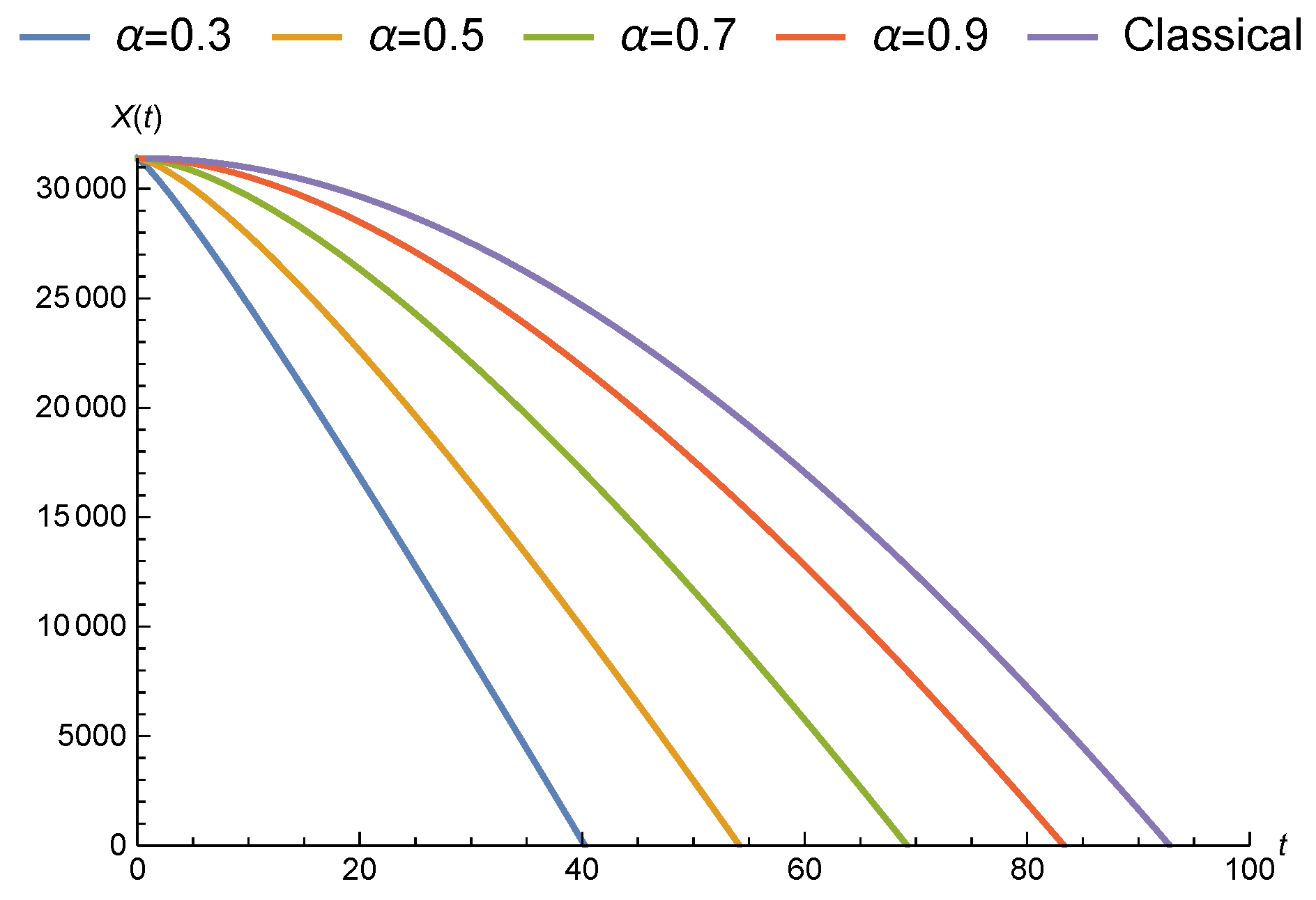
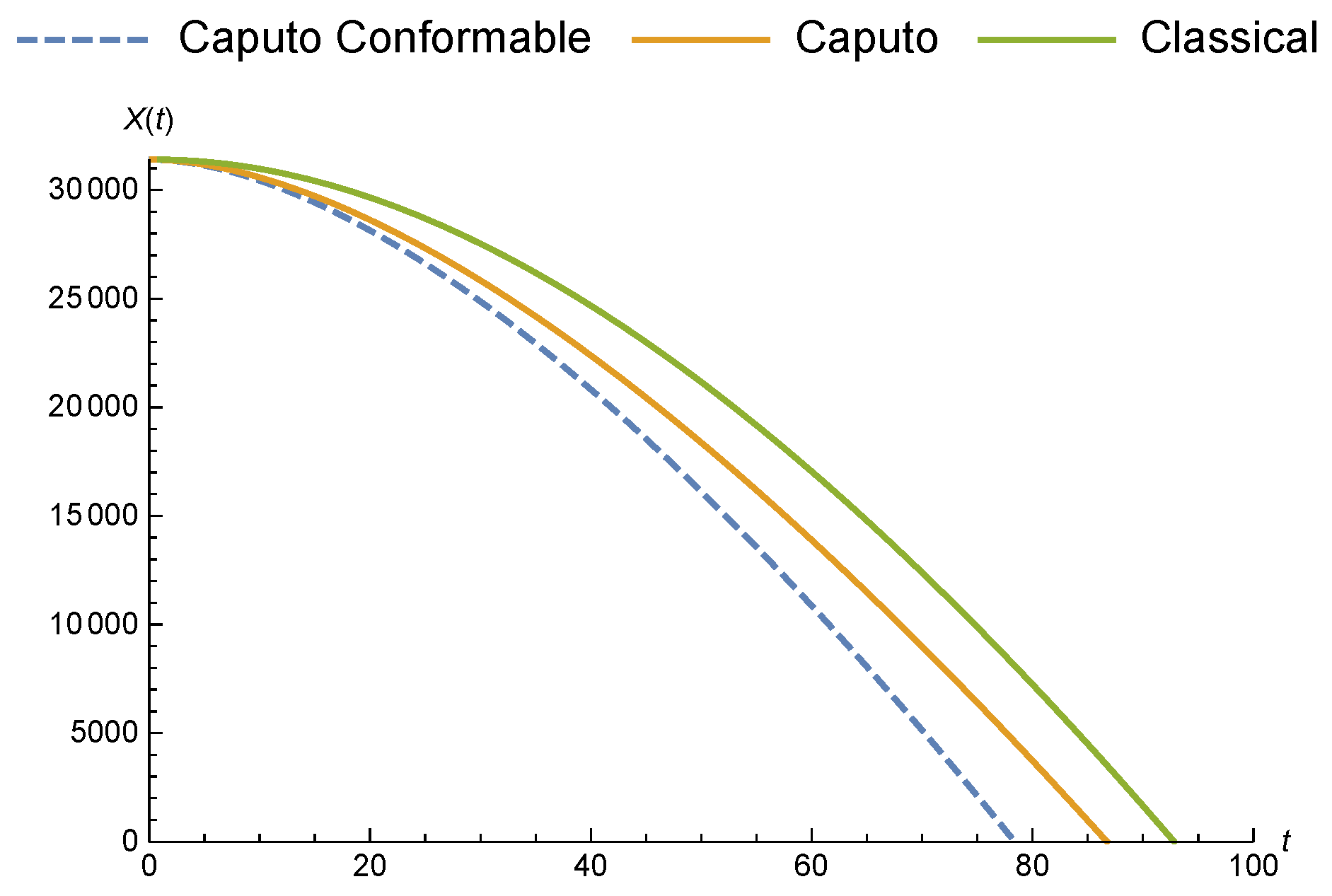
3.1. The Fractional Vertical Motion of a Falling Body Problem in a Resistant Medium

3.1.1. The Vertical Motion of a Falling Body Problem in a Resistant Medium with Liouville–Caputo Fractional Conformable Derivative

Let us consider Liouville-Caputo fractional conformable derivative, and obtain the analytical solution of the vertical motion of a falling body problem in a resistant medium. Taking the initial value problem

$$\begin{array}{ccc}\hfill m{\sigma }^{1-\alpha \beta }{}_0^{C\beta }{D}_t^{\alpha }v\left(t\right)& =& -mg-mkv\left(t\right),\hfill \end{array}$$

(11)

$$\begin{array}{ccc}\hfill v\left(0\right)& =& v_0.\hfill \end{array}$$

(12)

Solution 1.

We apply Picard successive approximation method for obtaining the analytical solution of the problem (11)–(12). So, let us apply the inverse operator of ${}_a^{C\beta }{D}_t^{\alpha }$ to Equation (11), we get

$${}_0^{\beta }{I}_t^{\alpha }\left({}_0^{C\beta }{D}_t^{\alpha }v\left(t\right)\right)=-{\sigma }^{\alpha \beta -1}{}_0^{\beta }{I}_t^{\alpha }\left\{g\right\}-{\sigma }^{\alpha \beta -1}{}_0^{\beta }{I}_t^{\alpha }\left(kv\left(t\right)\right).$$

Considering the Theorem 2 and the initial condition (12), we have

$$v\left(t\right)=v\left(0\right)-{\sigma }^{\alpha \beta -1}{}_0^{\beta }{I}_t^{\alpha }\left\{g\right\}-k{\sigma }^{\alpha \beta -1}\left({}_0^{\beta }{I}_t^{\alpha }\left(v\left(t\right)\right)\right).$$

Then

$$v_{i+1}\left(t\right)=v_0{-}_0^{\beta }{I}_t^{\alpha }\left\{g\right\}{\sigma }^{\alpha \beta -1}-k{\sigma }^{\alpha \beta -1}{}_0^{\beta }{I}_t^{\alpha }\left(v_i\left(t\right)\right),i=0,1,2,\dots$$

For $i=0,$ we can write

$$v_1\left(t\right)=v_0{-}_0^{\beta }{I}_t^{\alpha }\left(g\right){\sigma }^{\alpha \beta -1}-k{\sigma }^{\alpha \beta -1}\left({}_0^{\beta }{I}_t^{\alpha }\left(v_0\left(t\right)\right)\right)$$

(13)

where

$${}_0^{\beta }{I}_t^{\alpha }\left(v_0\left(t\right)\right)=\frac{v_0\left(t\right)}{\mathsf{\Gamma }\left(\beta \right)}\underset{0}{\overset{t}{\int }}{\left(\frac{t^{\alpha }-x^{\alpha }}{\alpha }\right)}^{\beta -1}\frac{dx}{x^{1-\alpha }}$$

Using the change of variable $u={\left(\frac{x-a}{t-a}\right)}^{\alpha },$ we have

$${}_0{I}_t^{\alpha }\left(v_0\right)=\frac{v_0{t}^{\alpha \beta }}{{\alpha }^{\beta }\mathsf{\Gamma }\left(\beta +1\right)}$$

(14)

Substituting Equation (14) into (13), we have

$$v_1\left(t\right)=v_0-\frac{g{t}^{\alpha \beta }{\sigma }^{\alpha \beta -1}}{{\alpha }^{\beta }\mathsf{\Gamma }\left(\beta +1\right)}-\frac{k{\sigma }^{\alpha \beta -1}{v}_0{t}^{\alpha \beta }}{{\alpha }^{\beta }\mathsf{\Gamma }\left(\beta +1\right)}.$$

For $i=1,$ we get

$$\begin{array}{ccc}\hfill v_2\left(t\right)& =& v_0{-}_0^{\beta }{I}_t^{\alpha }\left\{g\right\}{\sigma }^{\alpha \beta -1}-k{\sigma }^{\alpha \beta -1}{}_a^{\beta }{I}_t^{\alpha }\left\{v_1\left(t\right)\right\}\hfill \\ & =& v_0-\frac{g{t}^{\alpha \beta }{\sigma }^{\alpha \beta -1}}{{\alpha }^{\beta }\mathsf{\Gamma }\left(\beta +1\right)}-k{\sigma }^{\alpha \beta -1}{}_0^{\beta }{I}_t^{\alpha }\left\{v_0-\frac{g{t}^{\alpha \beta }{\sigma }^{\alpha \beta -1}}{{\alpha }^{\beta }\mathsf{\Gamma }\left(\beta +1\right)}-\frac{k{\sigma }^{\alpha \beta -1}{v}_0{t}^{\alpha \beta }}{{\alpha }^{\beta }\mathsf{\Gamma }\left(\beta +1\right)}\right\}\hfill \\ & =& v_0-\frac{g{t}^{\alpha \beta }{\sigma }^{\alpha \beta -1}}{{\alpha }^{\beta }\mathsf{\Gamma }\left(\beta +1\right)}-\frac{k{\sigma }^{\alpha \beta -1}{v}_0{t}^{\alpha \beta }}{{\alpha }^{\beta }\mathsf{\Gamma }\left(\beta +1\right)}+\frac{k{\left({\sigma }^{\alpha \beta -1}\right)}^{2}g{t}^{2\alpha \beta }}{{\alpha }^{2\beta }\mathsf{\Gamma }\left(2\beta +1\right)}+\frac{{\left(k{\sigma }^{\alpha \beta -1}\right)}^2{v}_0\left({}_0^{\beta }{I}_t^{\alpha }{t}^{\alpha \beta }\right)}{{\alpha }^{\beta }\mathsf{\Gamma }\left(\beta +1\right)}\hfill \end{array}$$

(15)

where ${}_0^{\beta }{I}_t^{\alpha }{\left(t-a\right)}^{\alpha \beta }={\displaystyle \frac{\mathsf{\Gamma }\left(\beta +1\right)t^{2\alpha \beta }}{{\alpha }^{\beta }\mathsf{\Gamma }\left(2\beta +1\right)}},$ then we can rewrite Equation (15)

$$\begin{array}{ccc}\hfill v_2\left(t\right)& =& v_0\left(1-\frac{k{\sigma }^{\alpha \beta -1}{t}^{\alpha \beta }}{{\alpha }^{\beta }\mathsf{\Gamma }\left(\beta +1\right)}+\frac{{\left(k{\sigma }^{\alpha \beta -1}\right)}^2{t}^{2\alpha \beta }}{{\alpha }^{2\beta }\mathsf{\Gamma }\left(2\beta +1\right)}\right)\hfill \\ & & -\frac{{\sigma }^{\alpha \beta -1}g{t}^{\alpha \beta }}{{\alpha }^{\beta }}\left(\frac{1}{\beta \mathsf{\Gamma }\left(\beta \right)}-\frac{k{\sigma }^{\alpha \beta -1}{t}^{\alpha \beta }}{{\alpha }^{\beta }2\beta \mathsf{\Gamma }\left(2\beta \right)}\right)\hfill \end{array}$$

Proceeding inductively we have

$$\begin{array}{ccc}\hfill v_i\left(t\right)& =& v_0\left(1-\frac{k{\sigma }^{\alpha \beta -1}{t}^{\alpha \beta }}{{\alpha }^{\beta }\mathsf{\Gamma }\left(\beta +1\right)}+\frac{{\left(k{\sigma }^{\alpha \beta -1}\right)}^2{t}^{2\alpha \beta }}{{\alpha }^{2\beta }\mathsf{\Gamma }\left(2\beta +1\right)}-\dots \right)\hfill \\ & & -\frac{{\sigma }^{\alpha \beta -1}g{\left(t\right)}^{\alpha \beta }}{{\alpha }^{\beta }}\left(\frac{1}{\beta \mathsf{\Gamma }\left(\beta \right)}-\frac{k{\sigma }^{\alpha \beta -1}{t}^{\alpha \beta }}{{\alpha }^{\beta }2\beta \mathsf{\Gamma }\left(2\beta \right)}+\dots \right)\hfill \\ & =& v_0\sum _{z=0}^i\frac{{\left(-1\right)}^z{\left(k{\sigma }^{\alpha \beta -1}\right)}^z{t}^{z\alpha \beta }}{{\alpha }^{z\beta }\mathsf{\Gamma }\left(z\beta +1\right)}-\frac{{\sigma }^{\alpha \beta -1}g{t}^{\alpha \beta }}{{\alpha }^{\beta }}\sum _{z=0}^i\frac{{\left(-1\right)}^z{\left(k{\sigma }^{\alpha \beta -1}\right)}^z{t}^{z\alpha \beta }}{{\alpha }^{z\beta }\left(z+1\right)\beta \mathsf{\Gamma }\left(z\beta +\beta \right)}.\hfill \end{array}$$

Therefore, as $i\to \infty$, we find the velocity as follows,

$$v\left(t\right)=v_0{E}_{\beta }\left(-\frac{k{\sigma }^{\alpha \beta -1}}{{\alpha }^{\beta }}{t}^{\alpha \beta }\right)-\frac{{\sigma }^{\alpha \beta -1}g{t}^{\alpha \beta }}{{\alpha }^{\beta }}\sum _{z=0}^{\infty }\frac{{\left(-k{\sigma }^{\alpha \beta -1}{t}^{\alpha \beta }\right)}^z}{{\alpha }^{z\beta }\left(z+1\right)\beta \mathsf{\Gamma }\left(z\beta +\beta \right)},$$

from here we get vertical distance of falling body in a resistant medium as follows

$$X\left(t\right)=h+v_{0}t{E}_{\beta ,2}\left(-\frac{k{\sigma }^{\alpha \beta -1}}{{\alpha }^{\beta }}{t}^{\alpha \beta }\right)-\frac{{\sigma }^{\alpha \beta -1}g{t}^{\alpha \beta +1}}{{\alpha }^{\beta }}\sum _{z=0}^{\infty }\frac{{\left(-k{\sigma }^{\alpha \beta -1}{t}^{\alpha \beta }\right)}^z}{\left[\left(z+1\right)\alpha \beta +1\right]{\alpha }^{z\beta }\left(z+1\right)\beta \mathsf{\Gamma }\left(z\beta +\beta \right)},$$

(16)

where $E_{\beta ,2}\left(t\right)$ is Mittag-Leffler function [21].

Now, let’s consider the different type of Liouville–Caputo fractional conformable derivatives defined in [2]. We obtain the analytical solution of the vertical motion of a falling body problem in a resistant medium. Considering the initial value problem

$$\begin{array}{ccc}\hfill {}_a^{AC\beta }{D}^{\alpha }v\left(t\right)& =& -mg-mkv\left(t\right),\hfill \\ \hfill v\left(0\right)& =& v_0.\hfill \end{array}$$

Solution 2.

If we apply similar arguments used in the proof of Problem (11)–(12), then we have

$$\begin{array}{ccc}\hfill X\left(t\right)& =& h+v_0(t+\frac{a}{\mathsf{\Gamma }\left(\alpha \right)})E_{\beta ,2}\left(-\frac{k{\sigma }^{\alpha \beta -1}}{{\alpha }^{\beta }}{(t+\frac{a}{\mathsf{\Gamma }\left(\alpha \right)})}^{\alpha \beta }\right)\hfill \\ & & -\frac{{\sigma }^{\alpha \beta -1}g{(t+\frac{a}{\mathsf{\Gamma }\left(\alpha \right)})}^{\alpha \beta +1}}{{\alpha }^{\beta }}\sum _{z=0}^{\infty }\frac{{\left(-k{\sigma }^{\alpha \beta -1}{(t+\frac{a}{\mathsf{\Gamma }\left(\alpha \right)})}^{\alpha \beta }\right)}^z}{\left[\left(z+1\right)\alpha \beta +1\right]{\alpha }^{z\beta }\left(z+1\right)\beta \mathsf{\Gamma }\left(z\beta +\beta \right)}.\hfill \end{array}$$

3.1.2. Vertical Motion of Falling Body Problem in a Resistant Medium with Liouville–Caputo Fractional Derivative

Now, let’s consider to the model of the vertical motion of a falling body problem in a resistant medium with the Liouville–Caputo fractional operator in [22] for comparing to Solution (16),

$$\begin{array}{ccc}\hfill m{\sigma }^{1-\alpha }{}_0^C{D}_t^{\alpha }v\left(t\right)& =& -mg-mkv\left(t\right),\hfill \\ \hfill v\left(0\right)& =& v_0.\hfill \end{array}$$

Taking direct and inverse Laplace transform to the equation above, we have analytical solutions

$$v\left(t\right)=-\frac{g}{k}+\left(v_0+\frac{g}{k}\right)E_{\alpha }\left(-k{\sigma }^{\alpha -1}{t}^{\alpha }\right),$$

$$X\left(t\right)=h-\frac{gt}{k}+\left(v_0+\frac{g}{k}\right)t{E}_{\alpha ,2}\left(-k{\sigma }^{\alpha -1}{t}^{\alpha }\right).$$

We observe the vertical motion of a falling body in the resistant medium with Liouville–Caputo conformable fractional derivative taking $v\left(0\right)=5$ m/s, $k=0.01$ s${}^{-1}$, $g=9.8$ m/s${}^2,$ h = 31,400 m in Figure 1, Figure 2, Figure 3 and Figure 4.

Figure 1. Analysis of the vertical motion of a falling body in a resistant medium under different orders while $\beta =0.9$.

Figure 2. Comparative analysis of the vertical motion of a falling body with different types of derivatives while $\alpha =0.95,\beta =0.95$.

Figure 3. Comparative analysis of the vertical motion of a falling body with different types of derivatives while $\alpha =0.8,\beta =1$.

Figure 4. Analysis of the vertical motion of a falling body in a resistant medium under different orders while $\alpha =0.9$.

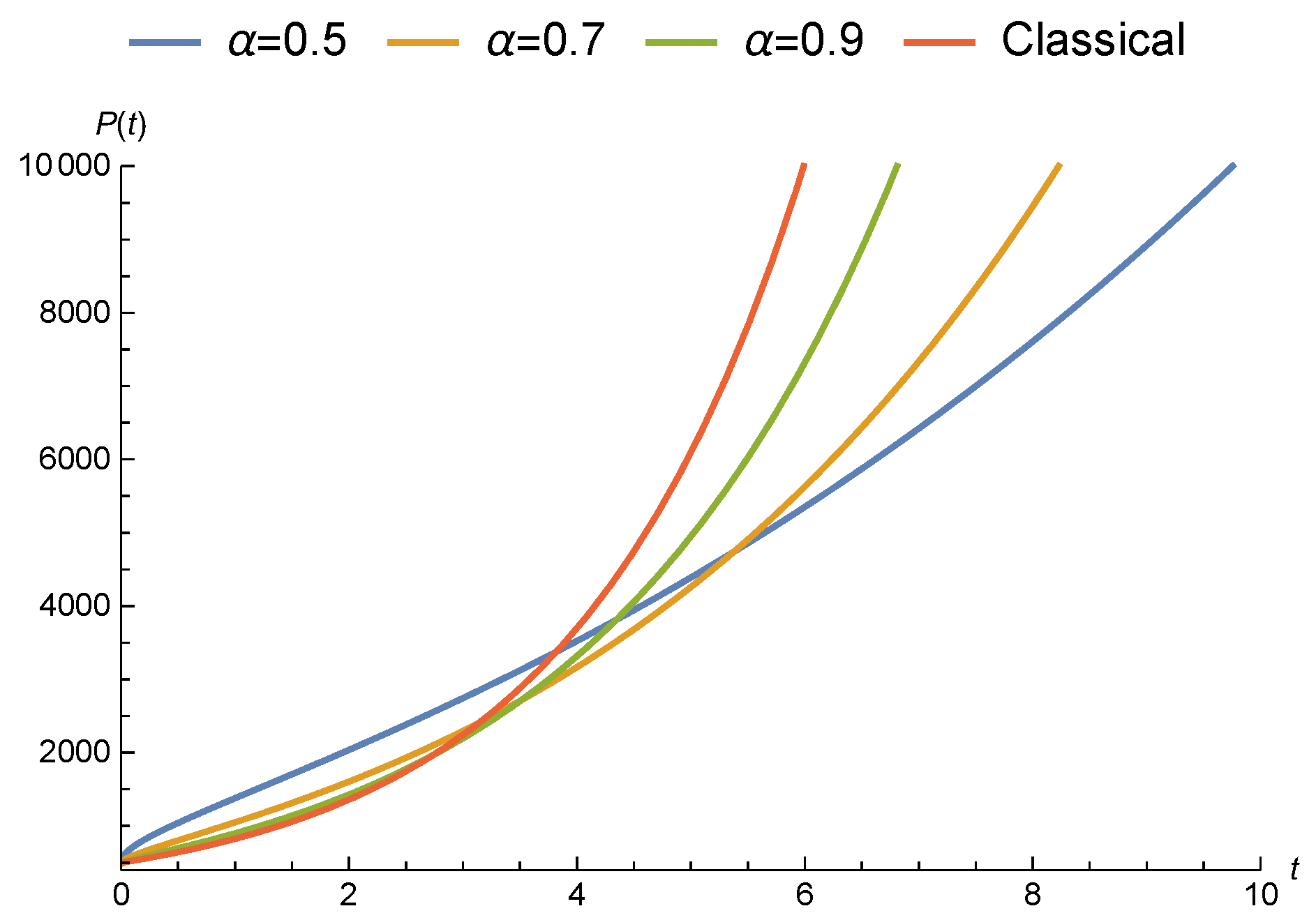
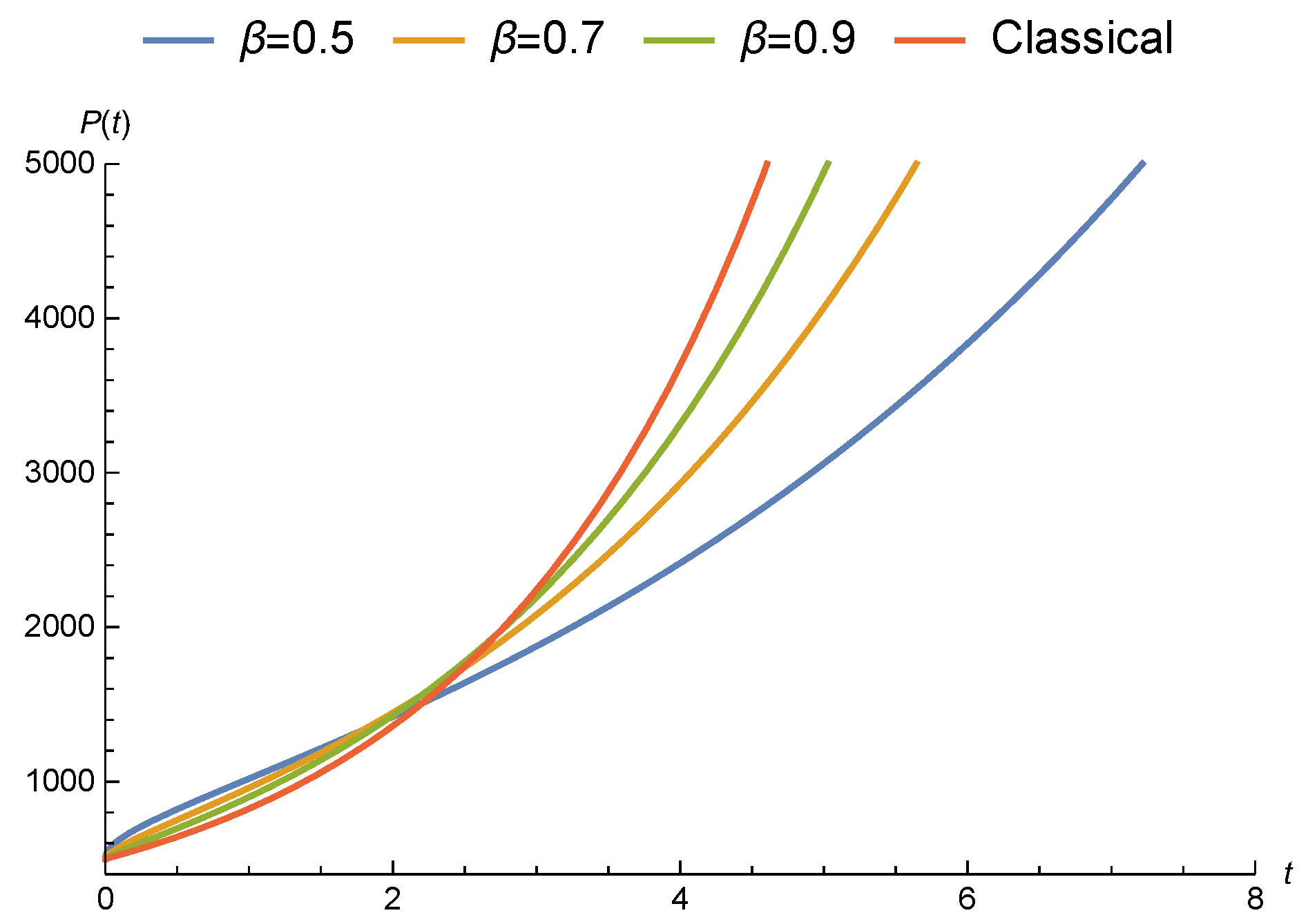
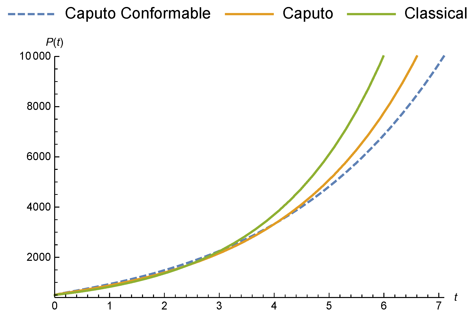
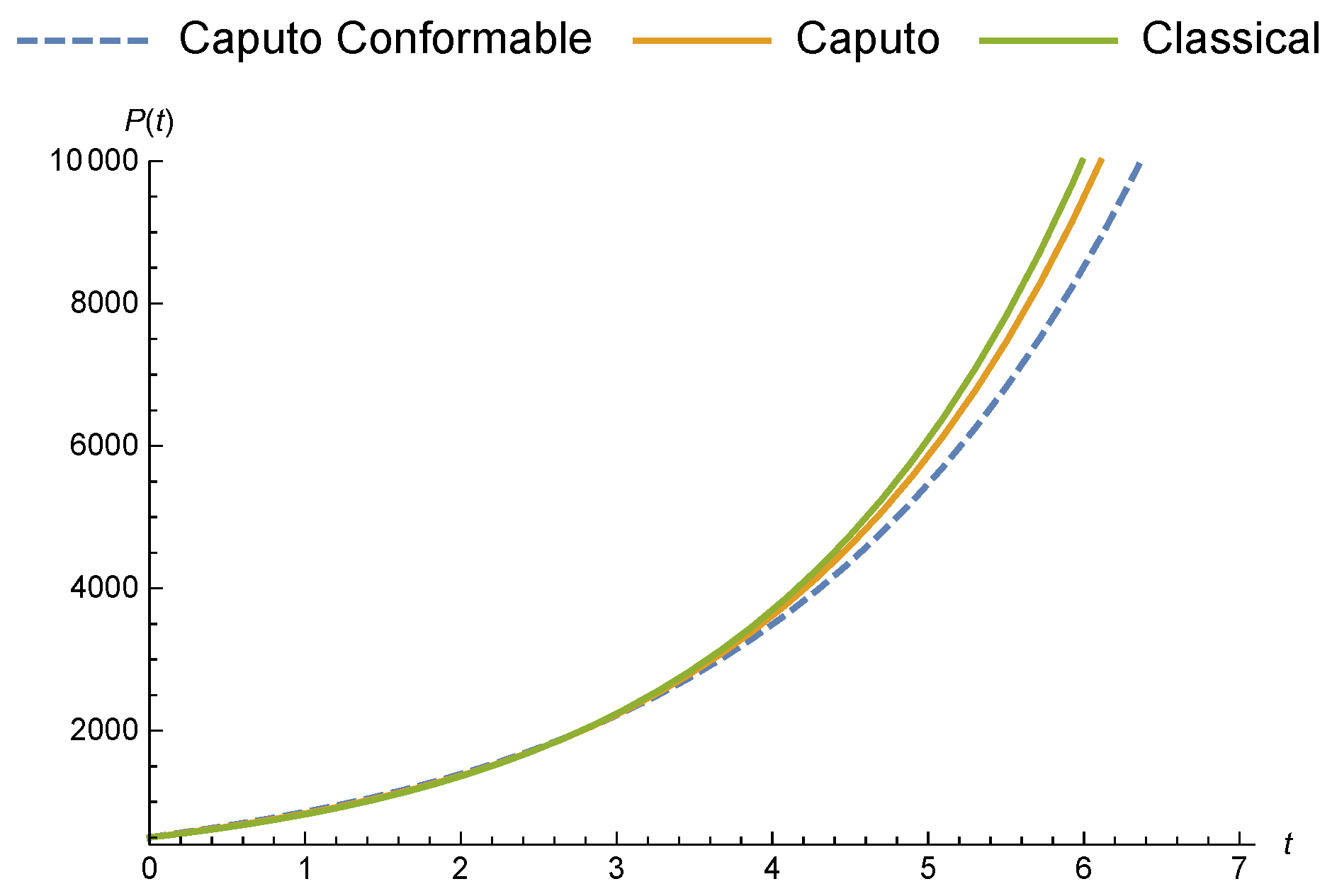
3.2. Fractional Malthusian Growth Model

3.2.1. Malthusian Growth Model with Liouville–Caputo Fractional Conformable Derivative

Let us consider the Liouville-Caputo fractional conformable derivative, and obtain the analytical solution of Malthusian growth model. Considering the initial value problem

$$\begin{array}{ccc}\hfill {}_a^{C\beta }{D}_t^{\alpha }P\left(t\right)& =& kP\left(t\right),\alpha >0,0<\beta \le 1,\hfill \end{array}$$

(17)

$$\begin{array}{ccc}\hfill P\left(a\right)& =& P_0.\hfill \end{array}$$

(18)

where $P\left(t\right)$ denote the population at time t, k is a positive constant.

Solution 3.

Let’s apply the Picard successive approximation method for obtaining the analytical solution of the problem (17) and (18). So, applying the inverse operator of ${}_a^{C\beta }{D}_t^{\alpha }$ to Equation (17), we get

$${}_a^{\beta }{I}_t^{\alpha }\left({}^{C\beta }{D}_t^{\alpha }P\left(t\right)\right)={}_a^{\beta }{I}_t^{\alpha }\left(kP\left(t\right)\right).$$

Considering the Theorem 2 and the initial condition (18), we have

$$P\left(t\right)=P\left(a\right){+}_a^{\beta }{I}_t^{\alpha }\left(kP\left(t\right)\right).$$

Then

$$P_{n+1}\left(t\right)=P_0+k_0^{\beta }{I}_t^{\alpha }\left(P_n\left(t\right)\right),n=0,1,2,\dots$$

For $n=0,$ we can write

$$P_1\left(t\right)=P_0+k_0^{\beta }{I}_t^{\alpha }\left(P_0\left(t\right)\right)$$

(19)

where

$${}_a^{\beta }{I}_t^{\alpha }\left(P_0\right)=\frac{P_0}{\mathsf{\Gamma }\left(\beta \right)}\underset{a}{\overset{t}{\int }}{\left(\frac{{\left(t-a\right)}^{\alpha }-{\left(x-a\right)}^{\alpha }}{\alpha }\right)}^{\beta -1}\frac{dx}{{\left(x-a\right)}^{1-\alpha }}.$$

Applying the change of variable $u={\left(\frac{x-a}{t-a}\right)}^{\alpha },$ we have

$$I_t^{\alpha }\left(P_0\right)=\frac{P_0{\left(t-a\right)}^{\alpha \beta }}{{\alpha }^{\beta }\mathsf{\Gamma }\left(\beta +1\right)}$$

(20)

Substituting Equation (20) into (19), we have

$$P_1\left(t\right)=P_0+\frac{k{P}_0{\left(t-a\right)}^{\alpha \beta }}{{\alpha }^{\beta }\mathsf{\Gamma }\left(\beta +1\right)}.$$

For $n=1,$ we get

$$\begin{array}{ccc}\hfill P_2\left(t\right)& =& P_0+k_a^{\beta }{I}_t^{\alpha }\left(P_1\right)\hfill \\ & =& P_0+k_a^{\beta }{I}_t^{\alpha }\left\{\left(P_0+\frac{k{P}_0{\left(t-a\right)}^{\alpha \beta }}{{\alpha }^{\beta }\mathsf{\Gamma }\left(\beta +1\right)}\right)\right\}\hfill \\ & =& P_0+\frac{k{P}_0{\left(t-a\right)}^{\alpha \beta }}{{\alpha }^{\beta }\mathsf{\Gamma }\left(\beta +1\right)}+\frac{k^2{P}_0}{{\alpha }^{\beta }\mathsf{\Gamma }\left(\beta +1\right)}{}_a^{\beta }{I}_t^{\alpha }\left\{{\left(t-a\right)}^{\alpha \beta }\right\},\hfill \end{array}$$

(21)

where $\left({}_a^{\beta }{I}_t^{\alpha }{\left(t-a\right)}^{\alpha \beta }\right)=\frac{\mathsf{\Gamma }\left(\beta +1\right){\left(t-a\right)}^{2\alpha \beta }}{{\alpha }^{\beta }\mathsf{\Gamma }\left(2\beta +1\right)},$ then we can rewrite Equation (21)

$$\begin{array}{cc}=& P_0+\frac{k{P}_0{\left(t-a\right)}^{\alpha \beta }}{{\alpha }^{\beta }\mathsf{\Gamma }\left(\beta +1\right)}+\frac{k^2{P}_0{\left(t-a\right)}^{2\alpha \beta }}{{\alpha }^{2\beta }\mathsf{\Gamma }\left(2\beta +1\right)}\hfill \\ =& P_0\left(1+\frac{k{\left(t-a\right)}^{\alpha \beta }}{{\alpha }^{\beta }\mathsf{\Gamma }\left(\beta +1\right)}+\frac{k^2{\left(t-a\right)}^{2\alpha \beta }}{{\alpha }^{2\beta }\mathsf{\Gamma }\left(2\beta +1\right)}\right).\hfill \end{array}$$

Proceeding inductively we have

$$\begin{array}{ccc}\hfill P_n\left(t\right)& =& P_0\left(1+\frac{k{\left(t-a\right)}^{\alpha \beta }}{{\alpha }^{\beta }\mathsf{\Gamma }\left(\beta +1\right)}+\frac{k^2{\left(t-a\right)}^{2\alpha \beta }}{{\alpha }^{2\beta }\mathsf{\Gamma }\left(2\beta +1\right)}+\dots \right)\hfill \\ & =& P_0\sum _{z=0}^n\frac{k^z{\left(t-a\right)}^{z\alpha \beta }}{{\alpha }^{z\beta }\mathsf{\Gamma }\left(z\beta +1\right)}.\hfill \end{array}$$

Therefore, as $n\to \infty$, we find

$$P\left(t\right)=P_0{E}_{\beta }\left(\frac{k}{{\alpha }^{\beta }}{\left(t-a\right)}^{\alpha \beta }\right).$$

(22)

Now, let’s consider the different type of Liouville–Caputo fractional conformable derivatives defined in [2]. We obtain the analytical solution of Malthusian growth model. Considering the initial value problem

$$\begin{array}{ccc}\hfill {}_a^{AC\beta }{D}^{\alpha }P\left(t\right)& =& kP\left(t\right),\alpha >0,0<\beta \le 1,\hfill \\ \hfill P\left(a\right)& =& P_0.\hfill \end{array}$$

Solution 4.

If we apply similar arguments used in the proof of Problem (17)–(18), then we have

$$\begin{array}{c}\hfill P\left(t\right)=P_0{E}_{\beta }\left(\frac{k}{{\alpha }^{\beta }}{(t+\frac{a}{\mathsf{\Gamma }\left(\alpha \right)})}^{\alpha \beta }\right).\end{array}$$

3.2.2. Malthusian Growth Model with Liouville–Caputo Fractional Derivative

Now, let us consider the Malthusian growth model with the Liouville–Caputo fractional operator in [23] for comparing to Solution (22)

$$\begin{array}{ccc}\hfill {}_a^C{D}_t^{\alpha }P\left(t\right)& =& kP\left(t\right),0<\alpha \le 1,\hfill \\ \hfill P\left(0\right)& =& P_0.\hfill \end{array}$$

Taking direct and inverse Laplace transform to the equation above, we have the analytical solution

$$x\left(t\right)=P_0{E}_{\alpha }\left(k{t}^{\alpha }\right).$$

We observe Malthusian growth model with Liouville–Caputo conformable fractional derivative taking $x\left(0\right)=500,$ $k=0.5$ in the Figure 5, Figure 6, Figure 7 and Figure 8.

Figure 5. Analysis of the Malthusian growth model under different orders while $\beta =0.9$.

Figure 6. Analysis of the Malthusian growth model under different orders while $\alpha =0.9$.

Figure 7. Comparative analysis of the Malthusian growth model with different types of derivatives while $\alpha =0.8,\beta =1$.

Figure 8. Comparative analysis of the Malthusian growth model with different types of derivatives while $\alpha =\beta =0.95$.

4. Conclusions

The vertical motion of a falling body in a resistant medium and the Malthusian growth model with a newly defined fractional conformable derivative are analyzed. The $\sigma$ auxiliary parameter is introduced for fractionalizing truly in view of physical comment of the vertical motion of a falling body problem. Analytical solutions of these modeling problems are found and shown by figures comparatively with the Liouville–Caputo fractional versions.

We observe the solution of the vertical motion of a falling body approaches to the classical case while $\alpha$ and $\beta$ approach to 1 in Figure 1 and Figure 2. Besides, we show the comparison of this problem with the Liouville–Caputo and classical cases while $\alpha ,$ $\beta$ approach to 1, and so, we observe that the solution converges to the Liouville–Caputo and classical case in Figure 3 and Figure 4.

We observe the solution of the Malthusian growth model approaches to the classical case while $\alpha$ and $\beta$ approach to 1 in Figure 5 and Figure 6, we show the comparison of this problem with the Liouville–Caputo and classical cases while $\alpha ,$ $\beta$ approach to 1, and we observe that the solution converges to the Liouville–Caputo and classical case in Figure 7 and Figure 8.

References

1. Jarad, F.; Uğurlu, E.; Abdeljawad, T.; Baleanu, D. On a new class of fractional operators. Adv. Differ. Equ. 2017, 2017, 247. [Google Scholar] [CrossRef]
2. Morales-Delgado, V.F.; Gómez-Aguilar, J.F.; Taneco-Hernandez, M.A. Analytical solutions of electrical circuits described by fractional conformable derivatives in Liouville–Caputo sense. AEU Int. J. Electron. Commun. 2018, 85, 108–117. [Google Scholar] [CrossRef]
3. Almeida, R. What is the best fractional derivative to fit data? arXiv, 2017; arXiv:1704.00609. [Google Scholar]
4. Ebaid, A.; Masaedeh, B.; El-Zahar, E. A new fractional model for the falling body problem. Chin. Phys. Lett. 2017, 34, 020201. [Google Scholar] [CrossRef]
5. Bas, E.; Ozarslan, R. Real world applications of fractional models by Atangana–Baleanu fractional derivative. Chaos Solitons Fractals 2018, 116, 121–125. [Google Scholar] [CrossRef]
6. Bas, E.; Acay, B.; Ozarslan, R. Fractional models with singular and non-singular kernels for energy efficient buildings. Chaos 2019, 29, 023110. [Google Scholar] [CrossRef] [PubMed]
7. Bas, E.; Ozarslan, R.; Baleanu, D.; Ercan, A. Comparative simulations for solutions of fractional Sturm–Liouville problems with non-singular operators. Adv. Differ. Equ. 2018, 2018, 350. [Google Scholar] [CrossRef]
8. Bas, E. The Inverse Nodal problem for the fractional diffusion equation. Acta Sci. Technol. 2015, 37, 2. [Google Scholar] [CrossRef]
9. Atangana, A.; Baleanu, D. New fractional derivatives with non-local and nonsingular kernel: Theory and application to heat transfer model. Therm. Sci. 2016, 20, 763–769. [Google Scholar] [CrossRef]
10. Hilfer, R. Applications of Fractional Calculus in Physics; World Scientific: Singapore, 2000. [Google Scholar]
11. Anatoly, A.K. Hadamard-type fractional calculus. J. Korean Math. Soc. 2001, 38, 1191–1204. [Google Scholar]
12. Caputo, M.; Fabrizio, M. A new definition of fractional derivative without singular kernel. Progr. Fract. Differ. Appl. 2015, 1, 1–13. [Google Scholar]
13. Abdeljawad, T. On conformable fractional calculus. J. Comput. Appl. Math. 2015, 279, 57–66. [Google Scholar] [CrossRef]
14. Atangana, A.; Baleanu, D.; Alsaedi, A. Analysis of time-fractional Hunter–Saxton equation: A model of neumatic liquid crystal. Open Phys. 2016, 14, 145–149. [Google Scholar] [CrossRef]
15. Khalil, R.; Al Horani, M.; Yousef, A.; Sababheh, M. A new definition of fractional derivative. J. Comput. Appl. Math. 2014, 264, 65–70. [Google Scholar] [CrossRef]
16. Anderson, D.R.; Ulness, D.J. Properties of the Katugampola fractional derivative with potential application in quantum mechanics. J. Math. Phys. 2015, 56, 063502. [Google Scholar] [CrossRef]
17. Abdeljawad, T.; Al-Mdallal, Q.M.; Jarad, F. Fractional logistic models in the frame of fractional operators generated by conformable derivatives. Chaos Solitons Fractals 2019, 119, 94–101. [Google Scholar] [CrossRef]
18. Abdeljawad, T. Fractional operators with boundary points dependent kernels and integration by parts. Discrete Contin. Dyn. Syst. Ser. S 2019, 1098–1107. [Google Scholar] [CrossRef]
19. Jarad, F.; Abdeljawad, T. Generalized fractional derivatives and Laplace transform. Discrete Contin. Dyn. Syst. Ser. S 2019, 1775–1786. [Google Scholar] [CrossRef]
20. Jarad, F.; Abdeljawad, T. Variational principles in the frame of certain generalized fractional derivatives. Discrete Contin. Dyn. Syst. Ser. S 2019, 574–582. [Google Scholar] [CrossRef]
21. Podlubny, I. Fractional Differential Equations; Academic Press: San Diego, CA, USA, 1999. [Google Scholar]
22. Garcia, J.R.; Calderon, M.G.; Ortiz, J.M.; Baleanu, D.; de Santiago, C.S.V. Motion of a particle in a resisting medium using fractional calculus approach. Proc. Rom. Acad. A 2013, 14, 42–47. [Google Scholar]
23. Almeida, R.; Bastos, N.R.; Monteiro, M.T.T. Modeling some real phenomena by fractional differential equations. Math. Methods Appl. Sci. 2016, 39, 4846–4855. [Google Scholar] [CrossRef]
24. Baskonus, H.M.; Bulut, H. Regarding on the prototype solutions for the nonlinear fractional-order biological population model. AIP Conf. Proc. 2016, 1738, 290004. [Google Scholar]
25. Yavuz, M.; Ozdemir, N.; Baskonus, H.M. Solutions of partial differential equations using the fractional operator involving Mittag-Leffler kernel. Eur. Phys. J. Plus 2018, 133, 215. [Google Scholar] [CrossRef]