Homotopy Perturbation ρ-Laplace Transform Method and Its Application to the Fractional Diffusion Equation and the Fractional Diffusion-Reaction Equation

Abstract

In this paper, the approximate solutions of the fractional diffusion equations described by the fractional derivative operator were investigated. The homotopy perturbation Laplace transform method of getting the approximate solution was proposed. The Caputo generalized fractional derivative was used. The effects of the orders $\alpha$ and $\rho$ in the diffusion processes was addressed. The graphical representations of the approximate solutions of the fractional diffusion equation and the fractional diffusion-reaction equation both described by the Caputo generalized fractional derivative were provided.

1. Introduction

Fractional calculus has many applications in physics and has attracted several researchers. The popularity of fractional calculus is due to the variety of the fractional derivatives operators. We can cite: the Caputo fractional derivative and the Riemann–Liouville fractional derivative [1,2], the Atangana–Baleanu fractional derivative [3,4,5,6], the Caputo–Fabrizio fractional derivative [7], and many others. The Atangana–Baleanu fractional derivative and the Caputo–Fabrizio fractional derivative were recently used in modeling physical phenomena [5,7,8,9,10,11]. The Atangana–Baleanu fractional derivative and the Caputo–Fabrizio fractional derivative are great compromises in modeling real world phenomena. The most relevant application of fractional calculus in physics is the fractional diffusion equation. In Reference [1], Podlubny introduced the diffusion equation using the fractional derivative operators. In Reference [12], Santoz studied the Fokker–Planck equation using the Atangana–Baleanu fractional derivative and the Caputo–Fabrizio fractional derivative. In Reference [13], Santoz used the fractional Prabhakar Derivative for studying the diffusion equation. In Reference [14], Santoz proposed a new approach of the random walk with the fractional diffusion equation. In Reference [7], Hristov gave a complete review of the fractional models and suggests a novel method for solving fractional diffusion equations.

The problem of solving differential equations is one of the most important field in fractional calculus. Many methods are used for getting the analytical solutions [15], the numerical solutions [16], and the approximate solutions. We have the Fourier sine transform [15,17]. We have the classical Laplace transform. We have the standard power series. We have the homotopy method [18,19] and others. Liao introduced the homotopy method in Reference [20]. The technique is favorite a favorite today for getting the approximate solutions of the fractional differential equations described by the fractional derivatives. Several results and applications of the homotopy method exist. In Reference [21], Das et al. solved the fractional diffusion equation described by the Caputo fractional derivative. They discussed the numerical results. They analyzed the convergence of the homotopy method. In Reference [18], Das et al. investigated getting the approximate solution of the fractional diffusion-reaction equation described by the Caputo fractional derivative. The authors used the optimal homotopy analysis method. They gave the graphical representations of the diffusion processes to illustrate the results. In Reference [22], Delgado et al. used the Laplace homotopy analysis for getting the approximate solutions of the linear partial differential equations described by the Caputo–Fabrizio fractional derivative and the Atangana–Baleanu fractional derivative. The main advancement of Delagado et al.’s work is the use of the Laplace transform in the application of the homotopy method. In Reference [23], Guo et al. presented the fractional variational homotopy perturbation iteration method. They applied their method for getting the solution of the fractional diffusion equation. They used the Riemann–Liouville fractional derivative in their studies. In Reference [24], Kumar et al. used the optimal homotopy analysis method for solving the nonlinear fractional diffusion equation described by the Caputo fractional derivative. In Reference [25], Yan used a modified perturbation homotopy method for getting the approximate solution of the fractional nonlinear heat transfer equation involving with the Caputo fractional derivative. Many other investigations exist relative to the homotopy methods, as in Abuasad [26] and Rajeev [27].

Other methods exist for solving the fractional diffusion equations. In Reference [28], Jassim et al. used the local fractional Laplace variational iteration method for solving the fractional diffusion equation and the fractional wave equation described by the local fractional derivative operators. In Reference [29], Khader et al. used the Legendre approximation for getting the approximate solution of the fractional diffusion-reaction equation. They considered the Caputo fractional derivative in their studies. In Reference [30], Hristov proposed the integral balance methods as the heat balance integral method and the double integral method for solving the fractional sub-diffusion equations.

Recently, the generalized fractional derivative was introduced in the literature by Udita [31]. Udita’s definition is the generalization of the Caputo and the Riemann–Liouville fractional derivative operators (see more investigations in [32,33,34]). In 2018, Fahd et al. introduced the Laplace transforms of the generalized fractional derivatives [35]. In our paper, we investigated the homotopy perturbation $\rho$-Laplace transform method for solving the fractional diffusion equation and the fractional diffusion-reaction equation described by the Caputo generalized fractional derivative. We used the Riemann–Liouville fractional integral in the classical homotopy perturbation method for solving the fractional differential equations. We had many iterations in the homotopy perturbation method. In all iterations, the Riemann–Liouville fractional integral was used for solving the fractional differential equations. The main difficulty in fractional calculus is to calculate the Riemann–Liouville fractional integral of a given function explicitly. It is not trivial and impossible in several cases. The novelty of the homotopy perturbation $\rho$-Laplace transform method is that, in all the iterations in our works, we replaced the Riemann–Liouville integrator by the $\rho$-Laplace transform for solving the fractional differential equations. This novel method was applied to solve the fractional diffusion equation and the fractional diffusion-reaction equation. We solved a classical open problem: getting the analytical solutions or approximates solutions of the diffusion equations. Note, many methods exist for solving the diffusion equations, such as the Fourier sine transform [36], the integral balance methods [30], the powers series, and many others. The application of the techniques cited above depends on the used boundary conditions. The methods have some limitations. In many cases, they cannot be applied. We proved our method is useful of getting the approximate solutions of the fractional diffusion equation and the fractional diffusion-reaction equation. The method takes into account the given boundary condition. The homotopy perturbation method has a history. The homotopy method was introduced by Liao [20]. Later, Shader et al. [37] proposed a modified version of the homotopy perturbation method. The authors in Reference [37] introduced a new interpretation of the parameter expansion in the homotopy perturbation method. Odibat et al. [38] applied the modified homotopy method for solving the fractional quadratic Riccati differential equation. Kumar et al. [39] applied the homotopy perturbation method for solving the fractional Black–Scholes European option pricing by using the Riemann–Liouville integral operator. See also Yavuz et al. [19]. Darzi et al. [40] proposed a new version of the homotopy perturbation method. The authors in Reference [40] introduced the fractional power series in the homotopy perturbation method. In our method, we proposed the $\rho$-Laplace transform for solving the fractional differential equations.

In Section 2, we recall the preliminary definitions and the functions for future use in the paper. In Section 3, we describe the homotopy Laplace transform method for solving the fractional differential equation represented by the Caputo generalized fractional derivative. In Section 4, we use the homotopy perturbation Laplace transform method for solving the generalized fractional diffusion equation. We analyzed the impact of the orders $\alpha$ and $\rho$ in the diffusion processes. In Section 5, we use the homotopy perturbation Laplace transform method for solving the generalized fractional diffusion-reaction equation. In Section 6, we give the concluding remarks.

2. Preliminary Defintions and Lemmas

In this section, the generalized fractional integral, the left generalized fractional derivative, the $\rho$-Laplace transform, and the Mittag–Leffler function have been recalled.

The generalized fractional integral is recalled in the following definition. Let’s the function $g:[0,+\infty [⟶\mathbb{R}$. As in [35], the generalized integral of order $\alpha$, $\rho >0$ of the function g is defined in the form:

$$\left(I^{\alpha ,\rho }g\right)\left(t\right)=\frac{1}{\Gamma \left(\alpha \right)}{\int }_0^t{\left(\frac{t^{\rho }-s^{\rho }}{\rho }\right)}^{\alpha -1}g\left(s\right)\frac{ds}{s^{1-\rho }},$$

(1)

where $\Gamma (\dots )$ is the Gamma function, for a.e $t>0,$ and $0<\alpha <1$.

The generalized fractional derivative is recalled in the following definition. Let the function $g:[0,+\infty [⟶\mathbb{R}$. As in Reference [35], the left generalized fractional derivative of order $\alpha$, $\rho >0$ of the function g is defined in the form:

$$\left(D^{\alpha ,\rho }g\right)\left(t\right)=\left(I^{1-\alpha ,\rho }g\right)\left(t\right)=\frac{1}{\Gamma (1-\alpha )}\left(\frac{d}{dt}\right){\int }_0^t{\left(\frac{t^{\rho }-s^{\rho }}{\rho }\right)}^{-\alpha }g\left(s\right)\frac{ds}{s^{1-\rho }},$$

(2)

where $\Gamma (\dots )$ is the Gamma function, for a.e $t>0,$ and $0<\alpha <1$.

The Caputo generalized fractional derivative is recalled in the following definition. Let the function $g:[0,+\infty [⟶\mathbb{R}$. As in Reference [35], the Caputo generalized fractional derivative of order $\alpha$, $\rho >0$ of the function g is defined in the form:

$$\left(D_c^{\alpha ,\rho }g\right)\left(t\right)=\frac{1}{\Gamma (1-\alpha )}{\int }_0^t{\left(\frac{t^{\rho }-s^{\rho }}{\rho }\right)}^{-\alpha }{\gamma }^{n}g\left(s\right)\frac{ds}{s^{1-\rho }},$$

(3)

where $\Gamma (\dots )$ is the Gamma function, for a.e $t>0,$ $\gamma =t^{1-\rho }\frac{d}{dt}$ and $0<\alpha <1$.

For the rest of this paper, the Laplace transform will be used to help us in solving the fractional differential equations. The $\rho$-Laplace transform was recently introduced in the literature [35]. The $\rho$-Laplace transform of the Caputo generalized fractional derivative is expressed in the following form:

$${\mathcal{L}}_{\rho }\left\{\left(D_c^{\alpha ,\rho }g\right)\left(t\right)\right\}=s^{\alpha }{\mathcal{L}}_{\rho }\left\{g\left(t\right)\right\}-\sum _{k=0}^{n-1}{s}^{\alpha -k-1}\left({\gamma }^{k}g\right)\left(0\right).$$

(4)

Besides, the $\rho$-Laplace transform of a given function g is described in the form:

$${\mathcal{L}}_{\rho }\left\{g\left(t\right)\right\}\left(s\right)={\int }_0^{\infty }{e}^{-s\frac{t^{\rho }}{\rho }}g\left(t\right)\frac{dt}{t^{1-\rho }}.$$

(5)

As in Reference [41], the Mittag–Leffler function with two parameters is defined as follows:

$$E_{\alpha ,\beta }\left(z\right)=\sum _{k=0}^{\infty }\frac{z^k}{\Gamma (\alpha k+\beta )},$$

(6)

where $\alpha >0,$ $\beta \in \mathbb{R}$ and $z\in \mathbb{C}$. The classical exponential function is obtained with $\alpha =\beta =1.$

3. Homotopy Perturbation and Laplace Transform Method

In this section, we describe the homotopy perturbation method and $\rho$-Laplace transform. We will use this to get the solutions of the fractional diffusion and the fractional diffusion-reaction equation, both represented by the Caputo generalized fractional derivative. The homotopy perturbation method for solving the differential equation was first proposed by Liao in [20]. Here, we combined both the homotopy perturbation method and the $\rho$-Laplace transform. Let the fractional differential equation described by the Caputo generalized fractional derivative given by:

$$D_c^{\alpha ,\rho }u(x,t)+Lu(x,t)+Nu(x,t)=g(x,t),$$

(7)

with the initial boundary condition defined as $u(x,0)=f\left(x\right),$ where L represents the linear operator which contains the integer or non-integer derivative operators, N denotes the nonlinear operator, and the function g is considered as the input term.

The homotopy perturbation is defined as the following construction [20]:

$$D_c^{\alpha ,\rho }u(x,t)+p\left\{Lu(x,t)+Nu(x,t)-g(x,t)\right\}=0,$$

(8)

where $p\in \left[0,1\right]$ represents the homotopy perturbation parameter. It is straightforward to notice, when the parameter $p=0$, we recover the generalized fractional differential equation defined by:

$$D_c^{\alpha ,\rho }u(x,t)=0,$$

(9)

with the initial boundary condition defined as $u(x,0)=f\left(x\right)$. Note that when the parameter $p=1$, we obtained the fractional differential equation described by the Caputo generalized fractional derivative defined in Equation (7). We used the parameter p to expand the solution of the fractional differential Equation (7), in the following form:

$$u(x,t)=u_0(x,t)+p{u}_1(x,t)+p^2{u}_2(x,t)+p^3{u}_3(x,t)+\dots .$$

(10)

The next step is to put Equation (10) into Equation (7). The functions $u_0,u_1,u_2,u_3$, … are the solutions of the fractional differential equations described by the Caputo generalized fractional derivative:

$$\begin{array}{ccc}\hfill p^0& :& D_c^{\alpha ,\rho }{u}_0(x,t)=0;\hfill \\ \hfill p^1& :& D_c^{\alpha ,\rho }{u}_1(x,t)=-L{u}_0(x,t)-m_1\left(u_0(x,t)\right)+g(x,t);\hfill \\ \hfill p^2& :& D_c^{\alpha ,\rho }{u}_2(x,t)=-L{u}_1(x,t)-m_2(u_0(x,t),u_1(x,t));\hfill \\ \hfill p^3& :& D_c^{\alpha ,\rho }{u}_3(x,t)=-L{u}_2(x,t)-m_3(u_0(x,t),u_1(x,t),u_2(x,t))\hfill \\ \hfill ⋮& :& ⋮,\hfill \end{array}$$

(11)

where the functions $m_1,m_2,m_2$, … satisfy the following condition:

$$\begin{array}{ccc}\hfill m(u_0(x,t)& +& p{u}_1(x,t)+p^2{u}_2(x,t)+p^3{u}_3(x,t)+\dots )=m_1(\left(u_0(x,t)\right)\hfill \\ & +& p{m}_2(u_0(x,t),u_1(x,t))+p^2{m}_3(u_0(x,t),u_1(x,t),u_2(x,t))+\dots .\hfill \end{array}$$

At each step, we applied the $\rho$-Laplace transform of getting the functions $u_0,u_1,u_2,u_3$, …. The boundary conditions of the fractional differential equation (Equation (10)) are given respectively by:

$$u_1(x,0)=u_2(x,0)=u_3(x,0)=\dots =0.$$

(12)

4. Approximate Solution of the Fractional Diffusion Equation

This section addresses the approximate solution of the fractional diffusion equation described by the Caputo generalized fractional derivative. We used both the homotopy perturbation method and the $\rho$-Laplace transform of the Caputo generalized fractional derivative to get the approximate solution of the fractional diffusion equation. The fractional diffusion equation under consideration is expressed as the following form:

$$D_t^{\alpha ,\rho }u(x,t)=\frac{{\partial }^{2}u(x,t)}{\partial x^2},$$

(13)

with the initial boundary condition defined as for all $x>0$,

$$u(x,0)=e^x-1.$$

(14)

We notice the Taylor expansion of the boundary condition at order 1, and we recover the classical boundary condition. That is $u(x,0)=x$. In other words, Equation (14) is the general boundary condition of the fractional diffusion equation defined by Equation (13).

In the first step of the resolution, we solve the fractional differential equation described by the Caputo generalized fractional derivative, expressed as:

$$D^{\alpha ,\rho }{u}_0(x,t)=0,$$

(15)

with the initial boundary condition defined by $u_0(x,t)=e^x-1$. When we apply the $\rho$-Laplace transform to both sides of Equation (15), we obtain:

$$\begin{array}{ccc}\hfill s^{\alpha }{u}_0(x,s)-s^{\alpha -1}{u}_0(x,0)& =& 0\hfill \\ \hfill s^{\alpha }{u}_0(x,s)& =& s^{\alpha -1}{u}_0(x,0)\hfill \\ \hfill s^{\alpha }{u}_0(x,s)& =& s^{\alpha -1}\left(e^x-1\right)\hfill \\ \hfill u_0(x,s)& =& \frac{e^x-1}{s}.\hfill \end{array}$$

(16)

When we apply the inverse of $\rho$-Laplace transform to both sides of Equation (16), we obtain the analytical solution of Equation (15),

$$u_0(x,t)=e^x-1.$$

(17)

In the second step, we solve the fractional differential equation described by the Caputo fractional derivative expressed as:

$$\begin{array}{ccc}\hfill D^{\alpha ,\rho }{u}_1(x,t)& =& \frac{{\partial }^2{u}_0(x,t)}{\partial x^2}\hfill \\ & =& e^x,\hfill \end{array}$$

(18)

with the initial boundary condition defined by $u_1(x,t)=0$. We apply the $\rho$-Laplace transform to both sides of Equation (18), and we obtain:

$$\begin{array}{ccc}\hfill s^{\alpha }{u}_1(x,s)-s^{\alpha -1}{u}_1(x,0)& =& \frac{e^x}{s}\hfill \\ \hfill s^{\alpha }{u}_1(x,s)& =& \frac{e^x}{s}\hfill \\ \hfill u_1(x,s)& =& \frac{e^x}{s^{1+\alpha }}.\hfill \end{array}$$

(19)

When we apply the inverse of $\rho$-Laplace transform to both sides of Equation (19), we obtain the analytical solution of equation:

$$u_1(x,t)=\frac{e^x}{\Gamma \left(1+\alpha \right)}{\left(\frac{t^{\rho }}{\rho }\right)}^{\alpha }.$$

(20)

In the third step, we solve the fractional differential equation described by the Caputo fractional derivative expressed as:

$$\begin{array}{ccc}\hfill D^{\alpha ,\rho }{u}_2(x,t)& =& \frac{{\partial }^2{u}_1(x,t)}{\partial x^2}\hfill \\ & =& \frac{e^x}{\Gamma \left(1+\alpha \right)}{\left(\frac{t^{\rho }}{\rho }\right)}^{\alpha },\hfill \end{array}$$

(21)

with initial boundary condition defined by $u_2(x,t)=0$. We apply the $\rho$-Laplace transform to both sides of Equation (19), and we obtain:

$$\begin{array}{ccc}\hfill s^{\alpha }{u}_2(x,s)-s^{\alpha -1}{u}_2(x,0)& =& \frac{e^x}{s^{1+\alpha }}\hfill \\ \hfill s^{\alpha }{u}_2(x,s)& =& \frac{e^x}{s^{1+\alpha }}\hfill \\ \hfill u_2(x,s)& =& \frac{e^x}{s^{1+2\alpha }},\hfill \end{array}$$

(22)

When we apply the inverse of $\rho$-Laplace transform to both sides of Equation (19), we obtain the analytical solution of Equation (18),

$$u_2(x,t)=\frac{e^x}{\Gamma \left(1+2\alpha \right)}{\left(\frac{t^{\rho }}{\rho }\right)}^{2\alpha }.$$

(23)

We adopt the same reasoning in the other steps. Finally, the approximate solution of the fractional diffusion in Equation described by the Caputo generalized fractional derivative Equation (13), under the condition Equation (14), is given by:

$$\begin{array}{ccc}\hfill u(x,t)& =& \underset{p\to 1}{lim}\sum _{i=0}^n{p}^i{u}_i(x,t)\hfill \\ \hfill u(x,t)& =& u_0(x,t)+u_1(x,t)+u_2(x,t)+\dots \hfill \\ \hfill u(x,t)& =& e^x-1+\frac{e^x}{\Gamma \left(1+\alpha \right)}{\left(\frac{t^{\rho }}{\rho }\right)}^{\alpha }+\frac{e^x}{\Gamma \left(1+2\alpha \right)}{\left(\frac{t^{\rho }}{\rho }\right)}^{2\alpha }+\dots \hfill \\ \hfill u(x,t)& =& e^x\left[1+\frac{1}{\Gamma \left(1+\alpha \right)}{\left(\frac{t^{\rho }}{\rho }\right)}^{\alpha }+\frac{1}{\Gamma \left(1+2\alpha \right)}{\left(\frac{t^{\rho }}{\rho }\right)}^{2\alpha }+...\right]-1\hfill \\ \hfill u(x,t)& =& e^x{E}_{\alpha }\left({\left(\frac{t^{\rho }}{\rho }\right)}^{\alpha }\right)-1.\hfill \end{array}$$

(24)

The approximate solution of the fractional diffusion equation described by the Caputo generalized fractional derivative Equation (13) is given by:

$$u(x,t)=e^x{E}_{\alpha }\left({\left(\frac{t^{\rho }}{\rho }\right)}^{\alpha }\right)-1.$$

(25)

We can notice that when $\alpha =\rho =1$, we recover the analytical solution of the classical diffusion equation defined by:

$${\partial }_{t}u(x,t)=\frac{{\partial }^{2}u(x,t)}{\partial x^2},$$

(26)

with initial boundary conditions defined as for all $x>0$:

$$u(x,0)=e^x-1,$$

(27)

given by:

$$u(x,t)=e^{x+t}-1.$$

(28)

In Figure 1, we depict the approximate solution of the fractional diffusion equation described by the Caputo generalized fractional derivative in the space coordinates and the time, when $\alpha =0.5$ and $\rho =1$.

In Figure 2, we depict the approximate solution of the fractional diffusion equation described by the Caputo generalized fractional derivative in the space coordinates and the time, when $\alpha =1$ and $\rho =0.5$.

In Figure 3, we depict the approximate solution of the fractional diffusion equation described by the Caputo generalized fractional derivative, when $\alpha \le 1$, $\rho =1$ and $t=0.5$.

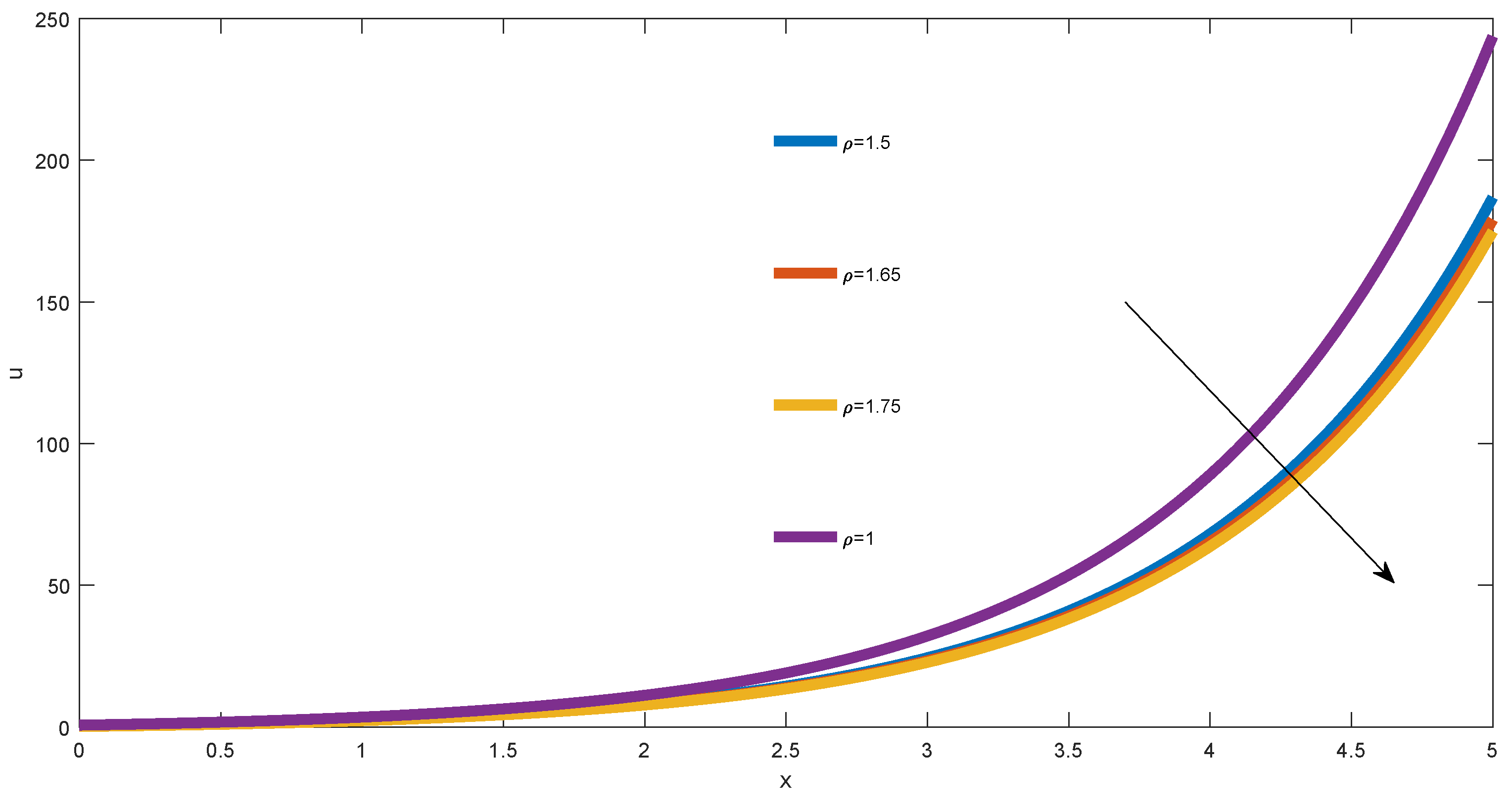
We observed all the curves increase and the order of the curves follow the increase of the order $\alpha$, (see the direction depicted by the arrow). In general, when we fixed the order $\rho =1$, we noticed an acceleration effect generated by the orders $\alpha \le 1$.

In Figure 4, we depict the approximate solution of the fractional diffusion equation described by the Caputo generalized fractional derivative, when $\alpha \ge 1$, $\rho =1$ and $t=0.5$. We observed all the curves increase and the order of the curves follow the increase of the order $\alpha$, so we have the same behaviors as in Figure 3. But in general, when we fixed the order $\rho =1$, we noticed a retardation effect generated by the orders $\alpha \ge 1$.

In Figure 5, we depict the approximate solution of the fractional diffusion equation described by the Caputo generalized fractional derivative, when $\rho \le 1$, $\alpha =1$ and $t=0.5$.

We observed all the curves increase and the order of the curves follow the increase of the order $\alpha$ (see the direction depicted by the arrow). In general, regarding the curve obtained with $\alpha =1$ and $\rho =1$, we notice an acceleration effect generated by the orders $\rho \le 1$.

In Figure 6, we depict the approximate solution of the fractional diffusion equation described by the Caputo generalized fractional derivative, when $\rho \ge 1$, $\alpha =1$ and $t=0.5$. We observed all the curves increase and the order of the curves follow the increase of the orders $\alpha$. In general, when we fixed the order $\alpha =1$, we noticed a retardation effect generated by the order $\rho \ge 1$.

5. Approximate Solutions of the Fractional Diffusion-Reaction Equation

This section addresses the approximate solution of the fractional diffusion-reaction equation described by the Caputo generalized fractional derivative. We used both the homotopy perturbation method and the Laplace transform of the Caputo generalized fractional derivative of getting the solution of the fractional diffusion-reaction equation. The fractional diffusion equation under consideration is expressed as:

$$D_t^{\alpha ,\rho }u(x,t)=\frac{{\partial }^{2}u(x,t)}{\partial x^2}+u(1-u),$$

(29)

with initial boundary condition defined as for all $x>0:$

$$u(x,0)=1/2.$$

(30)

In the first step of the resolution, we solve the fractional differential equation described by the Caputo generalized fractional derivative expressed as:

$$D^{\alpha ,\rho }{u}_0(x,t)=0,$$

(31)

with the initial boundary condition defined by $u_0(x,t)=1/2$. We apply the $\rho$-Laplace transform to both sides of Equation (31), and we obtain:

$$\begin{array}{ccc}\hfill s^{\alpha }{u}_0(x,s)-s^{\alpha -1}{u}_0(x,0)& =& 0\hfill \\ \hfill s^{\alpha }{u}_0(x,s)& =& s^{\alpha -1}{u}_0(x,0)\hfill \\ \hfill s^{\alpha }{u}_0(x,s)& =& \frac{1}{2}{s}^{\alpha -1}\hfill \\ \hfill u_0(x,s)& =& \frac{1}{2s}\hfill \end{array}$$

(32)

We apply the inverse of $\rho$-Laplace transform to both sides of Equation (32), and we obtain the analytical solution of Equation (31),

$$u_0(x,t)=\frac{1}{2}.$$

(33)

In the second step, we solve the fractional differential equation described by the Caputo fractional derivative expressed as:

$$\begin{array}{ccc}\hfill D^{\alpha ,\rho }{u}_1(x,t)& =& \frac{{\partial }^2{u}_0(x,t)}{\partial x^2}+u_0(1-u_0)\hfill \\ & =& \frac{1}{4},\hfill \end{array}$$

(34)

with initial boundary condition defined by $u_1(x,t)=0$. We apply the $\rho$-Laplace transform to both sides of Equation (34), and we obtain:

$$\begin{array}{ccc}\hfill s^{\alpha }{u}_1(x,s)-s^{\alpha -1}{u}_1(x,0)& =& \frac{1}{4s}\hfill \\ \hfill s^{\alpha }{u}_1(x,s)& =& \frac{1}{4s}\hfill \\ \hfill u_1(x,s)& =& \frac{1}{4s^{1+\alpha }}.\hfill \end{array}$$

(35)

We apply the inverse of $\rho$-Laplace transform to both sides of Equation (35), and we obtain the analytical solution of Equation (34),

$$u_1(x,t)=\frac{1}{4\Gamma \left(1+\alpha \right)}{\left(\frac{t^{\rho }}{\rho }\right)}^{\alpha }.$$

(36)

In the third step, we solve the fractional differential equation described by the Caputo generalized fractional derivative expressed as:

$$\begin{array}{ccc}\hfill D^{\alpha ,\rho }{u}_2(x,t)& =& \frac{{\partial }^2{u}_1(x,t)}{\partial x^2}+u_1(1-u_1)\hfill \\ & =& \frac{1}{4\Gamma \left(1+\alpha \right)}{\left(\frac{t^{\rho }}{\rho }\right)}^{\alpha }-{\left(\frac{1}{4\Gamma \left(1+\alpha \right)}\right)}^2{\left(\frac{t^{\rho }}{\rho }\right)}^{2\alpha },\hfill \end{array}$$

(37)

with the initial boundary condition defined by $u_2(x,t)=0$. We apply the $\rho$-Laplace transform to both sides of Equation (37), we obtain

$$\begin{array}{ccc}\hfill s^{\alpha }{u}_2(x,s)-s^{\alpha -1}{u}_2(x,0)& =& \frac{1}{4s^{1+\alpha }}-\frac{\Gamma \left(1+2\alpha \right)}{{\left(4\Gamma \left(1+\alpha \right)\right)}^2}\frac{1}{s^{1+2\alpha }}\hfill \\ \hfill s^{\alpha }{u}_2(x,s)& =& \frac{1}{4s^{1+\alpha }}-\frac{\Gamma \left(1+2\alpha \right)}{{\left(4\Gamma \left(1+\alpha \right)\right)}^2}\frac{1}{s^{1+2\alpha }}\hfill \\ \hfill u_2(x,s)& =& \frac{1}{4s^{1+2\alpha }}-\frac{\Gamma \left(1+2\alpha \right)}{{\left(4\Gamma \left(1+\alpha \right)\right)}^2}\frac{1}{s^{1+3\alpha }}\hfill \end{array}$$

(38)

We apply the inverse of $\rho$-Laplace transform to both sides of Equation (38), and we obtain the analytical solution of Equation (37),

$$u_2(x,t)=\frac{1}{4\Gamma \left(1+2\alpha \right)}{\left(\frac{t^{\rho }}{\rho }\right)}^{2\alpha }-\frac{\Gamma \left(1+2\alpha \right)}{{\left(4\Gamma \left(1+\alpha \right)\right)}^2}\frac{1}{\Gamma \left(1+3\alpha \right)}{\left(\frac{t^{\rho }}{\rho }\right)}^{3\alpha }.$$

(39)

We adopt the same reasoning in the other steps. Finally, the approximate solution of the fractional diffusion equation described by the Caputo generalized fractional derivative Equation (29), is given by:

$$\begin{array}{ccc}\hfill u(x,t)& =& \underset{p\to 1}{lim}\sum _{i=0}^n{p}^i{u}_i(x,t)\hfill \\ \hfill u(x,t)& =& u_0(x,t)+u_1(x,t)+u_2(x,t)+\dots \hfill \\ \hfill u(x,t)& =& \frac{1}{4}+\frac{1}{4}{E}_{\alpha }\left({\left(\frac{t^{\rho }}{\rho }\right)}^{\alpha }\right)-\frac{\Gamma \left(1+2\alpha \right)}{{\left(4\Gamma \left(1+\alpha \right)\right)}^2}\frac{1}{\Gamma \left(1+3\alpha \right)}{\left(\frac{t^{\rho }}{\rho }\right)}^{3\alpha }-\dots .\hfill \end{array}$$

(40)

The approximate solution of the fractional diffusion equation described by the Caputo generalized fractional derivative Equation (29) is given by:

$$u(x,t)=\frac{1}{4}+\frac{1}{4}{E}_{\alpha }\left({\left(\frac{t^{\rho }}{\rho }\right)}^{\alpha }\right)-h\left(t\right),$$

(41)

where

$$h\left(t\right)=\frac{\Gamma \left(1+2\alpha \right)}{{\left(4\Gamma \left(1+\alpha \right)\right)}^2}\frac{1}{\Gamma \left(1+3\alpha \right)}{\left(\frac{t^{\rho }}{\rho }\right)}^{3\alpha }-\dots .$$

(42)

We can notice when $\alpha =\rho =1$, we recover the analytical solution of the considered diffusion equation given by

$$u(x,t)=\frac{1}{4}+\frac{1}{4}{e}^t-\frac{1}{48}{t}^3.$$

(43)

In Figure 7, we depict the curve of the analytical solution of the diffusion-reaction equation obtained when $\alpha =\rho =1$. We observed the curve increase in time.

6. Convergence Analysis of the Method

In this section, we analyze the stability and the convergence of the homotopy perturbation $\rho$-Laplace transform method. The solution of the fractional diffusion equation (Equation (13)) and the fractional diffusion-reaction equation (Equation (29)) converge when the series defined in Equation (24) and (40) converge. To study the convergence of the homotopy perturbation $\rho$-Laplace transform method, we defined the error function expressed as:

$$e(x,t)=\left|u_{exact}-u_{appro}\right|,$$

(44)

where the function $u_{exact}$ represents the exact solution and $u_{appro}$ represents the approximate solution of the fractional diffusion equation. For the illustration of the convergence, we consider the order $\alpha =\rho =1$. The exact solution is given by $u_{exact}=e^{x+t}-1$. The approximate solution is obtained with Equation (24), after three iterations. The results are consigned in

Table 1. Numerical values of the error function.

x	0	0.1	0.2	0.3	0.4
t	0.1	0.1	0.1	0.1	0.1
$u_{exact}$	0.10517	0.22140	0.34985	0.49182	0.64872
$u_{appro}$	0.10500	0.22121	0.34965	0.49159	0.64846
$e=\left|u_{exact}-u_{appro}\right|$	$1.7\times {10}^{-4}$	$1.9\times {10}^{-4}$	$2\times {10}^{-4}$	$2.3\times {10}^{-4}$	$2.6\times {10}^{-4}$

.

We noted the results were in good agreement. Thus, the convergence of the homotopy perturbation $\rho$-Laplace transform method converged.

7. Conclusion

In this paper, the approximate solutions of the fractional diffusion equation and the fractional diffusion-reaction equation, both described by the Caputo fractional derivative, were provided, using the homotopy perturbation method. The impact of the order $\alpha$ and $\rho$ in the diffusion processes was addressed. In general, the orders $\alpha$ and $\rho$ had retardation or an acceleration effect in the diffusion processes. The behavior of the solutions of the fractional diffusion equation and the fractional diffusion-reaction equations both described by the Caputo fractional derivative in coordinate space and time were provided graphically. The problem of getting the analytical solution or the approximate solution of the fractional nonlinear sub-diffusion equation has been an open problem in fractional calculus. The problem is not trivial. Applying our method of combining both the homotopy perturbation method and the $\rho$-Laplace transform to get the approximate solution seemed adequate. We investigated using this method for solving this class fractional diffusion equations. In forthcoming works, some investigations will be done in this direction.