A Real-Time Vehicle Speed Prediction Method Based on a Lightweight Informer Driven by Big Temporal Data

Abstract

At present, the design of modern vehicles requires improving driving performance while meeting emission standards, leading to increasingly complex power systems. In autonomous driving systems, accurate, real-time vehicle speed prediction is one of the key factors in achieving automated driving. Accurate prediction and optimal control based on future vehicle speeds are key strategies for dealing with ever-changing and complex actual driving environments. However, predicting driver behavior is uncertain and may be influenced by the surrounding driving environment, such as weather and road conditions. To overcome these limitations, we propose a real-time vehicle speed prediction method based on a lightweight deep learning model driven by big temporal data. Firstly, the temporal data collected by automotive sensors are decomposed into a feature matrix through empirical mode decomposition (EMD). Then, an informer model based on the attention mechanism is designed to extract key information for learning and prediction. During the iterative training process of the informer, redundant parameters are removed through importance measurement criteria to achieve real-time inference. Finally, experimental results demonstrate that the proposed method achieves superior speed prediction performance through comparing it with state-of-the-art statistical modelling methods and deep learning models. Tests on edge computing devices also confirmed that the designed model can meet the requirements of actual tasks.

1. Introduction

Nowadays, as a key component of smart cities, smart transportation systems have attracted widespread attention from researchers around the world. Intelligent transportation systems (ITSs) [1,2,3] can optimize the organization and management of urban road network traffic, improve the efficiency of urban road network traffic, and are also the most effective measures to alleviate urban road traffic congestion without changing existing road facilities. Moreover, the development of intelligent transportation systems not only facilitates people’s travel, but also effectively solves environmental pollution and reduces the occurrence of accidents [4,5]. With the development of intelligent transportation systems, the autonomous driving of cars has become a key development direction for the future, and it is inseparable from the accurate automatic prediction of car speed. The accurate modelling and prediction of vehicle speeds in urban traffic are crucial to urban intelligent transportation systems and have been widely used, such as driving safety warning [6,7,8], automatic driving [9,10], vehicle navigation [11,12,13], traffic management [14,15,16], etc.

Vehicle speed prediction [17] refers to the estimation and inference of vehicle speed sequences in the future period based on historical data and environmental modelling to help realize vehicle safety-assisted driving [18] and intelligent vehicle behavior decision analysis [19]. Therefore, it is necessary to collect and analyze historical vehicle driving data to develop a corresponding strategy. The earlier and more accurate the data are acquired, the better the decision will be. Through speed prediction methods, a future period of driving data can be transmitted to the vehicle decision-making system for analysis, so as to develop the best behavior strategy which is an indispensable part of the intelligent transportation system coordination and arrangement process [20]. In addition, predicting vehicle speeds in advance can reduce the fuel consumption of the vehicle and traffic accidents during vehicle driving and improve the stability and safety of the automatic driving system. Traffic management departments can use vehicle speed prediction methods to predict vehicle speeds, thereby optimizing the timing of traffic lights and reducing congestion and traffic accidents. In the field of logistics delivery, vehicle speed prediction can be used to predict the travel time and arrival time of delivery vehicles, thereby assisting enterprises in optimizing logistics and distribution plans, improving efficiency, and reducing costs. In short, vehicle speed prediction plays an important role in real life, helping us better manage traffic, improve road safety, optimize logistics delivery, and ensure driving safety.

Vehicle speed prediction in urban traffic [21] is different from traditional time series analysis and is influenced by time, space, and many other external factors, such as road conditions, traffic flow status, weather conditions, etc. The speed signals received by sensors have complex dynamic spatial and temporal correlations, which make accurate and real-time prediction of vehicle speeds in urban traffic challenging. Currently, the following four main categories of approaches are classified to solve the vehicle speed prediction task: global positioning system (GPS)-based methods, visual perception methods, vehicle dynamics methods, and machine learning methods. The GPS-based methods [22,23,24] use sensors such as GPS and inertial measurement units (IMUs) to measure the speed and position of a vehicle in real time to complete speed prediction. This type of method requires the usage of high-precision GPS instruments, which can achieve high accuracy while incurring expensive costs. However, the positioning accuracy of GPS data may not necessarily meet complex location conditions. Visual perception methods utilize [25,26,27,28] devices like cameras to obtain information about the vehicle’s surroundings and combine them with machine learning methods to perform speed prediction. This kind of method can predict the speed and direction of the vehicle but can be more influenced by factors such as weather and lighting intensity. Vehicle-dynamics-based methods [29,30,31,32] use vehicle dynamics to build a prediction model to predict the future speeds of vehicles, in which a large number of factors such as vehicle dynamics parameters and road conditions are required to be considered. Machine learning methods [33,34,35] are one of the most commonly used techniques for vehicle speed prediction. Through developing models such as deep neural networks (DNNs) [36], support vector machines (SVMs) [37], and random forests (RFs) [38], features are extracted from sensor data to build a speed prediction system. When current data are fed into the model, it can accurately predict the future vehicle speeds. Machine learning methods are the most mature and widely used vehicle speed prediction techniques, but they still face problems such as insufficient generalization ability across scenarios, limited inference efficiency, and long-term data dependence. The focus of the four categories of methods is different and there are also connections between them. The first two focus on the sources and modalities of data used for predicting vehicle speeds, while the latter focus on modelling methods.

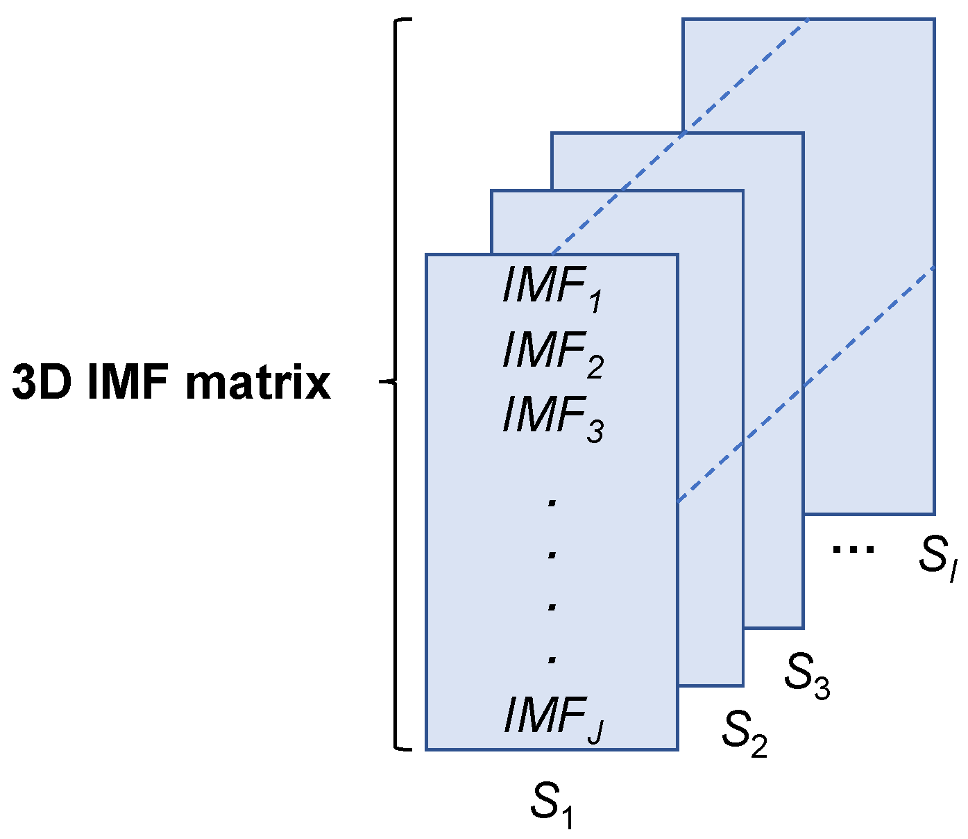
In this paper, we propose a real-time vehicle speed prediction method based on a lightweight deep learning model driven by big temporal data. Firstly, the temporal data collected by automotive sensors is decomposed into a feature matrix through empirical mode decomposition (EMD). Then, an informer model based on the attention mechanism is designed to extract key information for learning and prediction. During the iterative training process of the informer, redundant parameters are removed through importance measurement criteria to achieve real-time inference. Finally, experimental results demonstrate that the proposed method achieves superior speed prediction performance through comparing it with state-of-the-art statistical modelling methods and deep learning models. As a regression task, both accuracy and inference time pose challenges to the model. The design of a lightweight model structure helps to achieve vehicle speed prediction while being deployed in practical scenarios. To the best of our knowledge, this is the first attempt to develop and deploy a lightweight deep learning model specifically for temporal feature learning and real-time prediction of vehicle speeds and has been tested on the edge computing device EAIDK-310.

The remainder of the paper is organized as follows. In Section 2, we describe the related work of vehicle speed automatic prediction from two perspectives: traditional modelling methods and modern deep learning models. In Section 3, we introduce the lightweight informer model. The experimental results and analysis are reported in Section 4. Finally, we conclude with achievements, shortcomings, and future research directions in Section 5.

2. Related Work

In this section, we introduce the main related work used for the automatic prediction of vehicle speeds. The development trend is shown in Figure 1.

2.1. Traditional Modelling Methods

Shin and Sunwoo [39] proposed a vehicle speed prediction method based on a random model, which uses a Markov chain with speed constraints to generate speed trajectories under speed constraints. Experimental results illustrate that this method achieved a root mean square error of 3.8 km/h within a prediction range of up to 200 m. Jiang and Fei [40] used hidden Markov models (HMMs) to characterize the statistical relationship between vehicle speed and traffic flow and applied the forward–backward algorithm on HMMs to predict individual vehicle speeds. Jing et al. [41] utilizes an auto-regressive (AR) model to obtain the short-term dynamics of vehicle speed data and classifies the data into multiple acceleration states through fuzzy membership. During the prediction process, the acceleration measurement values are mapped to the Markov state through fuzzy coding, and the future acceleration state can be predicted through Markov transition. The Markov chain assumes that the probability distribution of the future state only depends on the current state, and has nothing to do with the past state, which is not satisfied with the long-term dependence in the time series data. Li et al. [42] demonstrated that combining the niche immunogenetic algorithm–support vector machine (NIGA-SVM) regression method on urban roads with the genetic algorithm–support vector machine (GA-SVM) regression method on suburban roads and highways can significantly improve the accuracy and timeliness of vehicle speed prediction. Since SVM is used to optimize the loss function through minimizing the edge interval and penalty factor, noise in the training dataset may have a drastic effect on the performance of the model. In addition, SVM is sensitive to parameters, such as kernel function type, kernel function parameters, and penalty factors. Amini et al. [43] proposed a comprehensive speed prediction framework based on historical traffic data classification and real-time V2I communication for the efficient energy management of electrified CAVs. To solve the problem of strong correlation factors being ignored in the context, Lv et al. [44] proposed an improved extreme gradient boost (XGBoost) speed prediction method. Shin et al. [45] proposed a speed prediction method based on a fuzzy Markov chain, which randomly predicts the speed of self-vehicles in the constrained region and solves the problem of increasing the model size when adding various input data. Rasyidi et al. [46] extracted features from real traffic data through considering adjacent links. After obtaining candidate features, linear regression, model tree, and k-nearest neighbor (K-NN) are all used for feature selection and speed prediction. However, traditional machine learning models such as K-NN and XGBoost simply classify or regress based on the characteristics of the data, so they may not be able to fully utilize the sequential information of the data.

Currently, a large number of modelling algorithms have been studied and developed for predicting vehicle speeds. Although multiple types of methods are considered in various scenarios, they all face the problem of insufficient generalization performance. In other words, once the application scenario becomes too complex (i.e., drivers exhibit unusual driving behavior when facing complex road conditions), the predictive performance of the algorithm significantly degrades. The parameter space and the corresponding decision boundary formed simply cannot cope with increasingly big data.

2.2. Modern Deep Learning Methods

Yan et al. [47] designed a deep neural network driven by five types of data (including historical vehicle speed, corresponding acceleration, steering information, position, and driving date) to predict future short-term vehicle speeds. Park et al. [48] proposed a speed prediction method based on neural network traffic modeling (NNTM-SP), which uses historical traffic data for training and predicts vehicle speed distribution driven by current traffic information. But they overlooked the potential impact of data type and structure on the prediction results. Lemieux [49] adopted deep learning technology to predict the specific speed curve of a single driver’s repeated driving cycle to minimize the fuel energy used during the journey. During the experiment, this work did not take into account complex driving behaviors and road conditions. Li et al. [50] proposed a novel speed prediction method based on the BP-LSTM model for long-term single speed prediction on a planned route. In addition, the Pearson correlation coefficient is used to analyze the correlation of historical feature parameters between driver vehicle road traffic and improve the computational efficiency of the model. Han et al. [51] combined a one-dimensional convolutional neural network with a bidirectional short-term memory network (CB-LSTM) and used the information provided by vehicle-to-vehicle (V2V) and vehicle-to-infrastructure (V2I) communications to complete the prediction of vehicle speeds. Shih et al. [52] designed a model consisting of an encoder, LSTM, and attention module to predict the movement of nearby vehicles through observing their movements in the last few seconds. Actually, multi-model fusion requires a large amount of computing resources; especially in cases with large amounts of data, the computational complexity will be higher, which will affect the real-time prediction ability of the model. In addition, the structure of the fusion model is relatively complex, making it difficult to explain the predicted results of the model, which may not be suitable for some application scenarios that require transparency.

Madhan et al. [53] established the architecture of a modular neural network (MNN) and obtained improved algorithms and corresponding parameters through training the dataset to improve the accuracy of vehicle speed prediction. Niu et al. [54] combined the U-Net and LSTM structures to construct a new spatio-temporal model L-U-Net, which can effectively predict the speed of urban-scale traffic conditions. Using spatio-temporal visual information and vehicle motion status, Zhang et al. [55] proposed an inflated 3-D inception LSTM network to predict short-term future vehicle speeds. Li et al. [56] proposed a method based on convolutional neural networks (CNNs) to better predict vehicle speeds. Jeong et al. [57] used a gated recursive unit (GRU) neural network driven by digital tachograph data (DTG) to predict vehicle speeds on highway. Three-dimensional deep learning models typically have high complexity and are prone to overfitting, resulting in poor generalization ability of the model. In general, 3D deep learning models require more feature engineering and higher requirements for data preprocessing. Considering the problem of data loss caused by device failures or abnormal data elimination, as well as the problem of data sparsity caused by small sample sizes, Zhao et al. [58] proposed a blank filling method based on historic trends to improve speed prediction performance. Compared with linear interpolation, this can better reflect the change trend of the signal. Maczyński et al. [59] developed an artificial neural network with radial neural functions driven by group parameters (i.e., average hourly traffic, the percentage of vehicles in free-flow traffic, geometric parameters of the road section (lane and hard shoulder width), and type of day and time) for predicting vehicle speeds. To reduce the errors of existing methods in short-term speed prediction and be able to predict medium- to long-term traffic speeds, Zhang et al. [60] proposed a traffic speed prediction method named ASTCN that combines attention and spatio-temporal features. The fusion of spatio-temporal features is of great help in characterizing the changing patterns of car speed, but accurately extracting spatio-temporal features separately is a challenge.

At present, a large number of deep learning models have been developed for vehicle speed prediction, with a focus on model structure and optimization methods, lacking targeted analysis of sensor signals. In fact, the effective extraction and learning of spatio-temporal features is the key to model generalization across different scenarios. Most work neglected data preprocessing, resulting in imprecise short-term vehicle speed prediction and failure of long-term predictions.

3. EMD-Based Informer for Vehicle Speed Prediction

In this section, we introduce the proposed EMD-based informer for vehicle speed prediction. Historical speed data is first decomposed into an intrinsic mode function (IMF) matrix via EMD to enhance its representativeness and then fed into the informer to extract critical features and make predictions for future vehicle speeds. The overall processing flow of the proposed method is shown in Figure 2.

3.1. EMD Analysis

3.1.1. Signal Decomposition

Considering a historical velocity dataset x(t)∈R^1×T that captures T moments, we first find all the maximum points and minimum points, and then fit the corresponding envelope e_max(t) and e_min(t) using the cubic spline function. The mean value of the upper and lower envelope can be calculated as follows:

$$e_1(t)=\frac{e_{\max }(t)+e_{\min }(t)}{2}$$

(1)

A new signal that removes low-frequency components can be obtained using the formula below:

$$p_1^1(t)=x(t)-e_1(t)$$

(2)

Then, Equation (2) is iterated k times until the IMF conditions (i.e., the difference in the number of extreme points and zero crossing points in the entire data length should not exceed one; the average value of the upper and lower envelope determined by the maximum and minimum points of cubic spline fitting is 0) are met, and the first-order IMF component can be expressed as follows:

$$IM{F}_1(t)=p_1^k(t)$$

(3)

In the subsequent decomposition process, a signal with the individual IMF components removed is continued iteratively through executing Equation (2) until the stopping criterion is satisfied:

$$SC=\frac{{\displaystyle \sum {\left|p_J^{k-1}(t)-p_J^k(t)\right|}^2}}{{\displaystyle \sum {[p_J^{k-1}(t)]}^2}}\le \epsilon$$

(4)

where ε is an artificially constrained small constant, such as 0.2. J represents the number of times the original signal is decomposed.

In other words, the signal after EMD can be represented as follows:

$$x(t)={\displaystyle \sum _{j=1}^{J}IM{F}_j(t)+r_J(t)}$$

(5)

where r_I(t) is the residual component with monotonicity.

To mitigate the mode mixing problem of EMD, we adopted multiple EMD decompositions with different noise introduced in the decomposition process to form a series of IMF sequences {S₁, S₂, …, S_I} where I is the number of introduced noises.

As a time-frequency domain signal processing method, EMD performs signal decomposition based on the time scale characteristics of the data itself, without any predefined basis functions. EMD has obvious advantages in processing non-stationary and non-linear data and is suitable for analyzing non-linear and non-stationary signal sequences with high signal-to-noise ratio (SNR).

3.1.2. Representation Construction

To improve the expressiveness of the signals, we combine multiple IMF sequences to form new signal representations that are used to guide the learning of deep learning models. Through adaptively weighting each IMF, a weighted three-dimensional IMF matrix can be obtained as the input, which is given by

$$\mathbf{X}=[{\lambda }_1{S}_1;{\lambda }_2{S}_2;\dots ;{\lambda }_I{S}_I]\in {ℝ}^{J\times I}$$

(6)

where [λ₁, λ₂,…, λ_I] are a set of learnable weighing parameters that determine the importance of each IMF sequence. The weighting parameters [λ₁, λ₂,…, λ_I] are usually initialized as average weighting factors, i.e., [1/I, 1/I, …, 1/I], to prevent learning with bias. As shown in Figure 3, the first and second dimensions of the constructed 3D IMF matrix reflect the time-domain and frequency-domain information, respectively, while the third dimension reflects the information at different scales.

The weighting feature allows each IMF to adjust the weighting factor to fit the model according to its importance. The advantage of this approach is that it can overcome the problem of different IMF scales while controlling the degree of contribution of each IMF to the features. Compared to treating each IMF as a feature vector, the IMF matrix can be constructed to fully utilize the information of each IMF. The problem of feature scaling imbalance that may result from the different scales of IMFs is avoided. In the constructed features, each IMF corresponds to a different time scale, which can capture the signal features on different time scales, thus improving the accuracy of timing prediction. Since each IMF is independent, even if some IMFs contain noise or outliers, other IMFs can still provide valid information, thus enhancing the robustness of the features. Features fused using multiple IMFs can characterize the signal more comprehensively, thus improving the generalization capability of the model and making it more capable of predicting vehicle speed in complex application scenarios.

3.2. Informer Model

3.2.1. Model Structure

The informer model consists of an encoder, a decoder, and a fully connected layer output. The specific model structure is shown in Figure 4. The encoder receives a long sequence input and obtains feature representations through a ProbSparse self-attention module and self-attention distillation module. The decoder receives the long sequence input and completes the learning and semantic understanding of encoded features through a multi-head attention module. Finally, the target is predicted and output directly through the fully connected layer.

In the encoder, the distilling operation is used to assign higher weights to dominant features with dominant attention, and a focus self-attention feature map is generated in the next layer, as given by

$$y_{i+1}^t=\mathrm{MaxPool}(\mathrm{ELU}(\mathrm{Conv}({\left[y_i^t\right]}_{\mathrm{AB}})))$$

(7)

where MaxPool(·), ELU(·), and Conv(·) denote the max-pooling, exponential linear unit activation function, and convolution operation, respectively. y_i and y_i+1 represent the feature map at i-th and (i+1)-th layer. [·]_AB is the attention block, in which the ProbSparse self-attention is defined as

$$\mathcal{A}(\mathbf{Q},\mathbf{K},\mathbf{V})=\mathrm{Softmax}(\frac{\overline{\mathbf{Q}}{\mathbf{K}}^{\mathrm{T}}}{\sqrt{d}})\mathbf{V}$$

(8)

where the attention function on a set of queries simultaneously is packed together into a matrix Q, and the keys and values are packed together into matrices K and V, respectively. d is the dimension of queries and keys.

In the decoder, a structure composed of two identical multi-head attention layers is used to attempt predictive inference for long sequences. Input is implemented through concatenation, as given by

$${\mathbf{X}}_{\mathrm{de}}^t=\mathrm{Concat}({\mathbf{X}}_{\mathrm{token}}^t,{\mathbf{X}}_0^t)$$

(9)

where X_token and X₀ are the start token and placeholder, respectively. The final output is obtained through a fully connected layer. Through jointly calculating the output through multiple heads, the output efficiency problem of the transformer in the long-term sequence prediction task can be solved.

In general, the informer model employs a multi-layer self-attentive mechanism that is able to reduce the dimensionality of time series data without losing information, thus improving the efficiency of the model. The self-attentive mechanism explicitly models the importance of each time step in the model and can provide interpretability. Moreover, the simultaneous consideration of features at different time scales makes it possible to model the time series more accurately. In practice, the informer model can automatically handle missing data and is flexible enough to cope with time series of different lengths and dimensions, making it suitable for various types of scenarios.

3.2.2. Parameters Learning

The principle of parameter importance is introduced to iteratively remove redundant parameters and perform fine-tuning, ensuring that the balance between parameter size and training loss meets the requirements. The final parameter scale is less than 1/10 of the original. The mean square error (MSE) is used as the loss function for measuring prediction performance on the target sequences, and the loss is propagated back from the decoder’s outputs across the entire model. The final output of the model is the vehicle speed at the next moment in the input sequence. During the training process of the informer, the parameters can be updated using the asynchronous stochastic gradient descent (SGD) method, as given by

$${\theta }^{t+1}={\theta }^t-{\gamma }_t\nabla f_{{\theta }^t,\mathbf{X}}$$

(10)

where

$${\theta }^1={\theta }^0-{\displaystyle \sum _{m=1}^M{\gamma }_{\mathrm{next}(1,m)}\nabla f({\theta }^0,{\mathbf{X}}_0)}$$

(11)

$${\gamma }_t={\gamma }_{\mathrm{next}(t+1,m_t)}$$

(12)

In the above equations, θ_t is the learnable parameters at the t-th training iteration, γ denotes the step size, m_k is the delay of the gradient at the t-th training iteration, and ▽f is the gradient. Unlike the naive SGD, the algorithm eventually performs an overall update due to asynchronous updates, where different layers are estimating the gradients of the outdated parameters in progress. During the training process, although a few severely outdated gradients are not enough to destroy the SGD’s performance, an asynchronous SGD performs better in this case. The pseudo-code of the asynchronous SGD optimization algorithm is shown in Algorithm 1.

Algorithm 1 Asynchronous SGD optimization process.

Input: Data sequence X

Initialization: Step size, initial parameters, and batch size.

Compute the batch gradient of D0.

for t = 1, 2, … do

Gradient arrives from batch set Dt;

Update the parameters;

Send θt to batch set Dt;

Compute the batch gradient of Dt.

end for

Output: Convergent deep learning model.

When using SGD-based optimization algorithms to update the parameters of deep learning models, the following aspects need to be taken into account to ensure good convergence and generalization:

• The learning rate controls the magnitude of parameter updates at each step; too fast of a learning rate may lead to model oscillation and non-convergence, while too slow of a learning rate will make the model converge slowly.
• The batch size controls the amount of data for each parameter update. Too large of a batch size may lead to insufficient memory, and too small of a batch size may make the model converge slowly.
• The SGD algorithm is sensitive to parameter initialization. Different initialization methods may lead to differences in model convergence speed and location. Considering that data from multiple scenarios are used for the experiments, random samples obeying a standard normal distribution were used to export the model parameters.
• Gradient explosion or gradient disappearance is a common problem faced by deep learning, which can be mitigated using gradient cropping techniques.

3.2.3. Vehicle Speed Prediction

Through continuous training iterations, when the converged lightweight deep learning model is obtained, it can be used to predict future vehicle speeds at T+1 moment driven by signals in the current time period T, as given by

$${\mathbf{Y}}_{T+1}=f^{*}[\mathbf{X}(t)]$$

(13)

where f* represents the convergent deep learning model. The pseudo-code of the entire process is shown in Algorithm 2.

In the application phase of the model, the trained model is converted to a format suitable for edge computing devices, and the model is deployed to edge computing devices. The vehicle speed sensor is built to collect the current speed of the vehicle in real time, input the collected historical vehicle speed data into the edge computing device, and use the deployed model to predict the future speed. Finally, the predicted results are fed back to the vehicle control system for adjusting vehicle speed and achieving intelligent control. It should be noted that the accuracy of the model and the real-time prediction of speed are key factors that need to be fully considered in the model design and deployment process. At the same time, the computing performance of edge computing devices also needs to be fully evaluated to ensure that the model can run on the device and achieve real-time prediction. In addition, the quality and real-time nature of data are also key factors affecting the accuracy of prediction, and sufficient preprocessing and cleaning of the data are needed to ensure the reliability of the prediction results.

Algorithm 2 Entire process for vehicle speed prediction.

Input: Data sequence X.

Initialization: The number of EMD, step size, initial model

parameters, and batch size.

Construct the 3D IMF matrix.

Initialize the deep learning model.

Train the model using the asynchronous SGD.

Crop the model to the lightweight structure.

Reasoning based on the forward propagation.

Output: Predicted vehicle speed at T + 1 moment.

4. Experimental Results and Analysis

In this section, we present the experiments conducted and report the corresponding results and analysis.

4.1. Experimental Settings

4.1.1. Experimental Data

The experiment used car driving data from three different scenarios, with a total of 60 h of speed signals. The signal acquisition process covers different time periods and road conditions to ensure the comprehensiveness and representativeness of the experimental data. Complex urban road conditions, rural roads, and rugged paths are considered in the experiments. Driving behavior is usually continuous to ensure predictability. Specifically, to ensure the accuracy and reliability of the data, the sampling frequency is set to 1 Hz, which means a total of 216,000 driving sample points have been collected. The driving signal categories include velocity, average velocity, idling time ratio, and accelerated velocity. Some examples of feature distributions in the vehicle motion process are shown in Figure 5.

The correlation between feature distributions is shown in Figure 6. Linear and nonlinear correlations, including Pearson, Spearman, and Kendall correlations, are calculated to observe the interrelationships between features. It can be observed that almost all the correlation measures among the features do not exceed 0.5 except for the autocorrelation on the diagonal, which shows a weak overall correlation. This means that the redundancy of feature is not significant and thus does not require the use of dimensionality reduction methods such as principal component analysis (PCA) for preprocessing. In contrast, the correlation under nonlinear measures like Spearman is more pronounced than that under linear measures. The vast majority of features between signals are not directly related, and deep learning models are needed to mine the underlying expert knowledge and construct potential mappings.

4.1.2. Experimental Hyper-Parameters

The hyper-parameters that need to be set manually during the experiments are summarized in

Table 1. Hyper-parameter settings of EMD-based informer.

Hyper-Parameters		Values
EMD	decomposition times I	6
	decomposition series J	5
Informer	step size	0.01
	batch size	16
	L2-regularization	0.0005
	dropout rate	0.5

, including decomposition times I and series J in EMD, and initial step size, batch size, L2-regularization intensity, and dropout rate in the informer. The decomposition times in EMD are empirically set to enhance decomposition stability while avoiding unnecessary computational complexity. Decomposing sequences are to ensure consistency in feature representation and avoid dimensional inconsistencies. The step size and batch size in deep learning have a significant impact on the training effectiveness and speed of the model. If the step size is too small, it will lead to slow model training speed and easily fall into local optimal solutions; excessive step size can lead to unstable model training, which may skip the optimal solution and cause oscillations. If the batch size is too small, it will lead to an inaccurate direction of model parameter updates and a poor training effect; too large of a batch size will lead to a slower training speed and increased memory occupation, which may lead to overfitting of the model. Generally, we conduct experiments to find the appropriate initial step size and batch size for the current model. L2-regularization is used to reduce the structural complexity of the model and improve its generalization ability. Dropout achieves the goal of improving generalization capability through suppressing the number of parameters in the last fully connected layer.

4.1.3. Experimental Platform

Under the condition of limited computational resources of vehicles, the capability to meet the performance requirements of inference accuracy and efficiency is the key to deciding whether the model can be deployed in practical applications. Experiments are performed using a workstation deployed in the cloud for training and the edge computing platform is deployed at the terminal for testing. The workstation consists of an NVIDIA RTX-3090 GPU, Intel I9-10920X CPU, 32 GB memory, 1 TB hard drive, and X299-Deluxe Prime. The EAIDK-310 is a powerful and easy-to-use AI development suite, which is suitable for various edge computing and AI application scenarios. The EAIDK-310 is powered by a Cortex-A53 CPU, Mali-450 MP2 GPU, 1 GB RAM, Bluetooth 5.0, 4× USB, and 1× Micro USB, as shown in Figure 7. The main chip of the EAIDK-310 is RK3228H equipped with a heterogeneous computing library, i.e., Arm SoC and HCL developed by OPEN AI LAB and Tengine, and can further accelerate mainstream neural networks.

4.1.4. Evaluation Metrics

To comprehensively evaluate the predictive performance of various methods, two types of evaluation metrics are counted. For predicting the vehicle speeds in the future T seconds, the absolute error (AE) and mean square error (MSE) of the method are defined as

$$\mathrm{AE}({\mathbf{X}}_i)=\frac{1}{T}{\displaystyle \sum _{j=1}^T\left|{\mathbf{Y}}^j-{\widehat{\mathbf{Y}}}^j\right|}$$

(14)

$$\mathrm{MSE}({\mathbf{X}}_i)=\frac{1}{T}{\displaystyle \sum _{j=1}^T{({\mathbf{Y}}^j-{\widehat{\mathbf{Y}}}^j)}^2}$$

(15)

where Y^j and ${\widehat{\mathbf{Y}}}^j$ are predicted and ground-truth vehicle speeds at the j-th future second. The MSE is usually used to evaluate the accuracy of predictive models, as it considers the distance between each predicted value and the true value. By contrast, the AE is usually used to evaluate the magnitude of measurement errors because it provides the average of all errors.

4.2. Prediction Performance

We first demonstrate the iterative training process of the objective function of the informer model, as shown in Figure 8. The optimization results of the original time-series-data-driven model and the 3D IMF matrix driven model are shown in Figure 8a,b, respectively. Both the models can converge to a stable position within 10 training epochs with a loss of less than 10⁻². It is worth noting that although the convergence iteration cycle of the 3D IMF driven model is longer, its corresponding loss value is smaller, which means that the corresponding model converges to a better location. Then, we report the changes in gradients and parameters during the optimization process to observe the convergence of the model under different drivers, as shown in Figure 9. In both cases, the gradient values gradually decrease with parameter updates, indicating that the models gradually converge to the position with a more refined loss landscape. The variance μ that gradually decreases during the whole training process reflects the stability of the optimization. When the loss of the validation set no longer decreases within six training epochs, the model of the current iteration period is used as the convergence model for testing. The vehicle speed prediction results of the convergence model are reported in Figure 10. Most prediction errors are concentrated within the range of −0.00883 to 0.02034. The error and response curves of prediction results are shown in Figure 11. It can be seen that significant changes in speed can easily lead to a decrease in prediction accuracy. To observe the predictive performance of the EMD-based informer more intuitively, we have sampled and compared the actual vehicle speeds with the predicted results, as shown in Figure 12. The method only experienced observable prediction errors at certain speed peaks.

Then, we compare the performance of a series of methods for predicting the vehicle speeds, in terms of inference accuracy and efficiency, including XGBoost [44], fuzzy Markov chain [45], NARX [61], LSTM [50], 1D CNN [56], and CNN-LSTM hybrid model [54]. The XGBoost [44], fuzzy Markov chain method [45], and NARX [61] use the default parameter settings of the machine learning toolbox. LSTM [50] is composed of an input gate, forget gate, cell, and output gate. Traffic congestion degree, road type, single travel distance, and speed limit are fed into the input gate, while the historical state information is fed into the forget gate. The hyper-parameter settings include: a dropout rate of 0.5, learning rate of 0.001, MAE loss, Adam optimizer, epoch of 100, and batch size of 1734. The 1D CNN model consists of one input layer, three convolutional layers, three max-pooling layers, one fully connected layer, and one output layer; all the convolution kernels are set to one dimension. The number and size of convolution kernels in the three convolutional layers are 256 × 1 × 3, 128 × 1 × 3, and 64 × 1 × 3, respectively. The hyper-parameters adopt the default settings under the classic AlexNet architecture. In CNN-LSTM, a spatial convolution model and an LSTM are connected in parallel, in which the CNN is composed of a contracting path, following the typical architecture of a convolutional network, and an expansive path. The learning rate equals 0.003, the L2 regularization coefficient equals 0.001, and other parameters are default parameters.

According to the results in

Table 2. Performance comparison of various vehicle speed prediction methods.

Methods	AE	MSE	Speed (s)
XGBoost	0.144	0.090	0.20
Markov	0.157	0.097	0.14
NARX	0.133	0.057	0.83
LSTM	0.118	0.039	1.30
1D CNN	0.127	0.052	0.22
CNN-LSTM	0.113	0.035	1.78
EMD-Informer	0.094	0.021	0.96

, although 1D CNN achieved the most advanced inference speed (0.22 s per signal), the EMD-based informer has achieved the best prediction accuracy with an AE of 0.094 and MSE of 0.021. The inference speed of 0.96 s per signal on edge devices of the EMD-based informer is able to meet the real-time requirements of practical applications. By comparison, LSTM performs better than CNN because the temporal information is more critical than the spatial information. The fusion of the two models can take into account the information of both, but it will lead to an increase in computational complexity with an inference time of 1.78 s. In addition, the performance of traditional modelling methods like XGBoost and Markov on complex temporal data is unsatisfactory, although they typically have lower structural complexity and higher inference speed.

4.3. Ablation Studies

In this section, we observed the vehicle speed prediction performance of the EMD-Informer model driven by different inputs through ablation studies, as shown in

Table 3. Performance comparison of EMD-based informer driven by different inputs.

Input Types	AE	MSE	Speed (s)
Time series input	0.133	0.069	0.15
Single IMF input	0.107	0.026	0.24
3D IMF matrix input	0.094	0.021	0.96

. Three types of inputs, including time series, single IMF, and 3D IMF matrix, are used for testing. Since the time series is not subjected to any pre-processing to help extract implicit expert knowledge, it requires the least amount of inference time (0.15 s per signal) but the lowest prediction accuracy (AE of 0.133 and MSE of 0.069). The single IMF input can effectively reduce the speed prediction error while bringing a small amount of inference time consumption. The 3D IMF matrix is able to achieve the best speed prediction accuracy while meeting the real-time requirements.

4.4. Robustness Analysis

Hyper-parameters determine the robustness of deep learning models for practical applications in a variety of different contexts. Therefore, we observed the speed prediction accuracy of the EMD-based informer under different hyper-parameter settings, including decomposition times I, decomposition series J, step size, and batch size, as shown in

Table 4. Performance comparison of EMD-based informer under different hyper-parameters.

Hyper-Parameters		AE	MSE
Types	Values
Decomposition times I	3	0.112	0.034
	4	0.110	0.032
	5	0.103	0.027
	6	0.094	0.021
Decomposition series J	2	0.104	0.024
	3	0.101	0.023
	4	0.096	0.021
	5	0.094	0.021
Step size	0.001	0.103	0.024
	0.005	0.092	0.019
	0.01	0.094	0.021
	0.05	0.128	0.060
Batch size	8	0.113	0.034
	16	0.094	0.021
	32	0.098	0.022
	64	0.090	0.017

. The number of decomposition times and decomposition series determine the size of the 3D IMF matrix, which also affects the speed prediction accuracy and inference efficiency of the informer. It can be seen that the prediction error gradually decreases as the values of both I and J increase. The step size and batch size affect the predictive performance of the converged model through influencing the optimization process. According to the experimental results, the effect of these hyper-parameters on the prediction error can be almost negligible. In practical applications, reasonable hyper-parameters can be set according to prior information to avoid their impacts as much as possible. Even if step size increases from 0.001 to 0.05, the changes in AE and MSE do not exceed 0.025 and 0.04, respectively. As batch size increases, the model prediction error gradually decreases, but this performance improvement is not significant. On the other hand, the optimization process caused by the increase in batch size increases the impact on memory.

5. Conclusions

Nowadays, automatic vehicle speed prediction based on artificial intelligence plays a positive role in promoting traffic safety, improving energy efficiency, promoting intelligent transportation, and achieving precise road condition monitoring. It is of great significance for accelerating transportation modernization, improving social and economic benefits, and promoting sustainable development. In this paper, we propose a real-time vehicle speed prediction method based on the lightweight deep learning model informer driven by big temporal data. To the best of our knowledge, this is the first attempt to develop and deploy a lightweight deep learning model specifically for temporal feature learning and real-time prediction of vehicle speeds and has been tested on the edge computing device EAIDK-310. For the regression task of predicting vehicle speed, we have taken into account both the prediction accuracy and inference speed of the deep learning model and verified its effectiveness through the actual collection of time series data in multiple scenarios. Compared with a series of deep learning models, the experimental results illustrate its superiority. Moreover, ablation studies have demonstrated its robustness in practical applications.

In fact, different road conditions, such as highways and rural roads, may lead to completely different driving patterns, which pose even greater challenges to predicting vehicle speed. The introduction of more types of sensor data helps to model driving behaviors under different road conditions. In the future, we plan to test the effectiveness of the proposed method on more complex road conditions (e.g., complex terrain like curves and rugged mountain roads, and varying degrees of traffic congestion) and improve the prediction accuracy of vehicle speeds through introducing more modal sensor data, such as vision and GPS. Detailed information about the test section, such as the speed limits of the area and the speed range recorded for each coordinate, will also be considered during the experimental process.

References

1. Wang, Y.; Gui, G.; Gacanin, H.; Ohtsuki, T.; Dobre, O.; Poor, H. An efficient specific emitter identification method based on complex-valued neural networks and network compression. IEEE J. Sel. Areas Commun. 2021, 39, 2305–2317. [Google Scholar] [CrossRef]
2. Wang, Y.; Gui, G.; Lin, Y.; Wu, H.-C.; Yuen, C.; Adachi, F. Few-Shot Specific Emitter Identification via Deep Metric Ensemble Learning. IEEE Internet Things J. 2022, 9, 24980–24994. [Google Scholar] [CrossRef]
3. Zheng, Q.; Tian, X.; Yang, M.; Wu, Y.; Su, H. CLMIP: Cross-layer manifold invariance based pruning method of deep convolutional neural network for real-time road type recognition. Multidimens. Syst. Signal Process. 2021, 32, 239–262. [Google Scholar] [CrossRef]
4. Li, Q.; Cheng, R.; Ge, H. Short-term vehicle speed prediction based on BiLSTM-GRU model considering driver heterogeneity. Phys. A Stat. Mech. Its Appl. 2023, 610, 128410. [Google Scholar] [CrossRef]
5. Peng, Y.; Hou, C.; Zhang, Y.; Lin, Y.; Gui, G.; Gacanin, H.; Mao, S.; Adachi, F. Supervised Contrastive Learning for RFF Identification with Limited Samples. IEEE Internet Things J. 2023. Early access. [Google Scholar] [CrossRef]
6. Pulvirenti, L.; Rolando, L.; Millo, F. Energy management system optimization based on an LSTM deep learning model using vehicle speed prediction. Transp. Eng. 2023, 11, 100160. [Google Scholar] [CrossRef]
7. Zhang, Y.; Peng, Y.; Sun, J.; Gui, G.; Lin, Y.; Mao, S. GPU-Free Specific Emitter Identification Using Signal Feature Embedded Broad Learning. IEEE Internet Things J. 2023, 10, 13028–13039. [Google Scholar] [CrossRef]
8. Fu, X.; Peng, Y.; Liu, Y.; Lin, Y.; Gui, G.; Gacanin, H.; Adachi, F. Semi-Supervised Specific Emitter Identification Method Using Metric-Adversarial Training. IEEE Internet Things J. 2023, 10, 10778–10789. [Google Scholar] [CrossRef]
9. Zheng, Q.; Yang, M.; Zhang, Q.; Yang, J. A bilinear multi-scale convolutional neural network for fine-grained object classification. IAENG Int. J. Comput. Sci. 2018, 45, 340–352. [Google Scholar]
10. Xu, T.; Xu, P.; Zhao, H.; Yang, C.; Peng, Y. Vehicle running attitude prediction model based on Artificial Neural Network-Parallel Connected (ANN-PL) in the single-vehicle collision. Adv. Eng. Softw. 2023, 175, 103356. [Google Scholar] [CrossRef]
11. Yuan, H.; Li, G. A Survey of Traffic Prediction: From Spatio-Temporal Data to Intelligent Transportation. Data Sci. Eng. 2021, 6, 63–85. [Google Scholar] [CrossRef]
12. Yin, X.; Wu, G.; Wei, J.; Shen, Y.; Qi, H.; Yin, B. Deep learning on traffic prediction: Methods, analysis, and future directions. IEEE Trans. Intell. Transp. Syst. 2021, 23, 4927–4943. [Google Scholar] [CrossRef]
13. Tian, X.; Zheng, Q.; Jiang, N. An abnormal behavior detection method leveraging multi-modal data fusion and deep mining. IAENG Int. J. Appl. Math. 2021, 51, 92–99. [Google Scholar]
14. Tedjopurnomo, D.A.; Bao, Z.; Zheng, B.; Choudhury, F.; Qin, A.K. A Survey on Modern Deep Neural Network for Traffic Prediction: Trends, Methods and Challenges. IEEE Trans. Knowl. Data Eng. 2020, 34, 1544–1561. [Google Scholar] [CrossRef]
15. Boukerche, A.; Wang, J. Machine Learning-based traffic prediction models for Intelligent Transportation Systems. Comput. Netw. 2020, 181, 107530. [Google Scholar] [CrossRef]
16. Zheng, Q.; Yang, M.; Tian, X.; Wang, X.; Wang, D. Rethinking the role of activation functions in deep convolutional neural networks for image classification. Eng. Lett. 2020, 28, 80–92. [Google Scholar]
17. Zhang, Q.; Yang, M.; Zheng, Q.; Zhang, X. Segmentation of hand gesture based on dark channel prior in projector-camera system. In Proceedings of the IEEE/CIC International Conference on Communications in China (ICCC), Qingdao, China, 22–24 October 2017; pp. 1–6. [Google Scholar]
18. Guo, K.; Hu, Y.; Qian, Z.; Liu, H.; Zhang, K.; Sun, Y.; Gao, J.; Yin, B. Optimized Graph Convolution Recurrent Neural Network for Traffic Prediction. IEEE Trans. Intell. Transp. Syst. 2020, 22, 1138–1149. [Google Scholar] [CrossRef]
19. Zheng, Q.; Zhao, P.; Wang, H.; Elhanashi, A.; Saponara, S. Fine-Grained Modulation Classification Using Multi-Scale Radio Transformer With Dual-Channel Representation. IEEE Commun. Lett. 2022, 26, 1298–1302. [Google Scholar] [CrossRef]
20. Zhao, L.; Song, Y.; Zhang, C.; Liu, Y.; Wang, P.; Lin, T.; Deng, M.; Li, H. T-GCN: A Temporal Graph Convolutional Network for Traffic Prediction. IEEE Trans. Intell. Transp. Syst. 2019, 21, 3848–3858. [Google Scholar] [CrossRef] [Green Version]
21. Goyani, J.; Chaudhari, P.; Arkatkar, S.; Joshi, G.; Easa, S.M. Operating Speed Prediction Models by Vehicle Type on Two-Lane Rural Highways in Indian Hilly Terrains. J. Transp. Eng. Part A: Syst. 2022, 148, 04022001. [Google Scholar] [CrossRef]
22. Niu, X.; Zhu, Y.; Zhang, X. DeepSense: A novel learning mechanism for traffic prediction with taxi GPS traces. In Proceedings of the IEEE Global Communications Conference, Austin, TX, USA, 8–12 December 2014; pp. 2745–2750. [Google Scholar]
23. Kuang, L.; Hua, C.; Wu, J.; Yin, Y.; Gao, H. Traffic Volume Prediction Based on Multi-Sources GPS Trajectory Data by Temporal Convolutional Network. Mob. Netw. Appl. 2020, 25, 1405–1417. [Google Scholar] [CrossRef]
24. Yang, H.; Zhang, X.; Li, Z.; Cui, J. Region-Level Traffic Prediction Based on Temporal Multi-Spatial Dependence Graph Convolutional Network from GPS Data. Remote. Sens. 2022, 14, 303. [Google Scholar] [CrossRef]
25. Ma, X.; Dai, Z.; He, Z.; Ma, J.; Wang, Y.; Wang, Y. Learning Traffic as Images: A Deep Convolutional Neural Network for Large-Scale Transportation Network Speed Prediction. Sensors 2017, 17, 818. [Google Scholar] [CrossRef] [Green Version]
26. Akolkar, H.; Ieng, S.H.; Benosman, R. Real-time high speed motion prediction using fast aperture-robust event-driven visual flow. IEEE Trans. Pattern Anal. Mach. Intell. 2020, 44, 361–372. [Google Scholar] [CrossRef] [PubMed]
27. Yu, B.; Chen, Y.; Bao, S. Quantifying visual road environment to establish a speeding prediction model: An examination using naturalistic driving data. Accid. Anal. Prev. 2019, 129, 289–298. [Google Scholar] [CrossRef] [PubMed]
28. Guan, Q.; Bao, H.; Xuan, Z. The research of prediction model on intelligent vehicle based on driver’s perception. Clust. Comput. 2017, 20, 2967–2979. [Google Scholar] [CrossRef]
29. Malaghan, V.; Pawar, D.S.; Dia, H. Speed prediction models for heavy passenger vehicles on rural highways based on an instrumented vehicle study. Transp. Lett. 2022, 14, 39–48. [Google Scholar] [CrossRef]
30. Zheng, Q.; Zhao, P.; Li, Y.; Wang, H.; Yang, Y. Spectrum interference-based two-level data augmentation method in deep learning for automatic modulation classification. Neural Comput. Appl. 2021, 33, 7723–7745. [Google Scholar] [CrossRef]
31. Mehdi, M.Z.; Kammoun, H.M.; Benayed, N.G.; Sellami, D.; Masmoudi, A.D. Entropy-based traffic flow labeling for CNN-based traffic congestion prediction from meta-parameters. IEEE Access 2022, 10, 16123–16133. [Google Scholar] [CrossRef]
32. George, M.A.; Kamat, D.V.; Kurian, C.P. Electric vehicle speed tracking control using an ANFIS-based fractional order PID controller. J. King Saud Univ. Eng. Sci. 2022. early access. [Google Scholar] [CrossRef]
33. Pan, Z.; Zhang, W.; Liang, Y.; Zhang, W.; Yu, Y.; Zhang, J.; Zheng, Y. Spatio-Temporal Meta Learning for Urban Traffic Prediction. IEEE Trans. Knowl. Data Eng. 2020, 34, 1462–1476. [Google Scholar] [CrossRef]
34. Diao, C.; Zhang, D.; Liang, W.; Li, K.-C.; Hong, Y.; Gaudiot, J.-L. A Novel Spatial-Temporal Multi-Scale Alignment Graph Neural Network Security Model for Vehicles Prediction. IEEE Trans. Intell. Transp. Syst. 2022, 24, 904–914. [Google Scholar] [CrossRef]
35. Tian, X.; Ruan, F.; Cheng, H.; Zheng, Q. A signal timing model for improving traffic condition based on active priority control strategy. Eng. Lett. 2020, 28, 235–242. [Google Scholar]
36. Zheng, Q.; Tian, X.; Yang, M.; Wu, Y.; Su, H. PAC-Bayesian framework based drop-path method for 2D discriminative convolutional network pruning. Multidimens. Syst. Signal Process. 2020, 31, 793–827. [Google Scholar] [CrossRef]
37. Tian, X.; Su, H.; Wang, F.; Zhang, K.; Zheng, Q. A electric vehicle charging station optimization model based on fully electrified forecasting method. Eng. Lett. 2019, 27, 731–743. [Google Scholar]
38. Zheng, Q.; Tian, X.; Liu, S.; Yang, M.; Wang, H.; Yang, J. Static hand gesture recognition based on Gaussian mixture model and partial differential equation. IAENG Int. J. Comput. Sci. 2018, 45, 569–583. [Google Scholar]
39. Shin, J.; Sunwoo, M. Vehicle Speed Prediction Using a Markov Chain With Speed Constraints. IEEE Trans. Intell. Transp. Syst. 2018, 20, 3201–3211. [Google Scholar] [CrossRef]
40. Jiang, B.; Fei, Y. Vehicle Speed Prediction by Two-Level Data Driven Models in Vehicular Networks. IEEE Trans. Intell. Transp. Syst. 2016, 18, 1793–1801. [Google Scholar] [CrossRef]
41. Jing, J.; Filev, D.; Kurt, A.; Ozatay, E.; Michelini, J.; Ozguner, U. Vehicle speed prediction using a cooperative method of fuzzy Markov model and auto-regressive model. In Proceedings of the IEEE Intelligent Vehicles Symposium (IV), Los Angeles, CA, USA, 11–14 June 2017; pp. 881–886. [Google Scholar]
42. Li, Y.; Chen, M.; Lu, X.; Zhao, W. Research on optimized GA-SVM vehicle speed prediction model based on driver-vehicle-road-traffic system. Sci. China Technol. Sci. 2018, 61, 782–790. [Google Scholar] [CrossRef]
43. Amini, M.R.; Feng, Y.; Yang, Z.; Kolmanovsky, I.; Sun, J. Long-term vehicle speed prediction via historical traffic data analysis for improved energy efficiency of connected electric vehicles. Transp. Res. Rec. 2020, 2674, 17–29. [Google Scholar] [CrossRef]
44. Lv, F.; Wang, J.; Cui, B.; Yu, J.; Sun, J.; Zhang, J. An improved extreme gradient boosting approach to vehicle speed prediction for construction simulation of earthwork. Autom. Constr. 2020, 119, 103351. [Google Scholar] [CrossRef]
45. Shin, J.; Kim, S.; Sunwoo, M.; Han, M. Ego-vehicle speed prediction using fuzzy Markov chain with speed constraints. In Proceedings of the IEEE Intelligent Vehicles Symposium (IV), Paris, France, 9–12 June 2019; pp. 2106–2112. [Google Scholar]
46. Rasyidi, M.A.; Kim, J.; Ryu, K.R. Short-term prediction of vehicle speed on main city roads using the k-nearest neighbor algorithm. J. Intell. Inf. Syst. 2014, 20, 121–131. [Google Scholar] [CrossRef] [Green Version]
47. Yan, M.; Li, M.; He, H.; Peng, J. Deep Learning for Vehicle Speed Prediction. Energy Procedia 2018, 152, 618–623. [Google Scholar] [CrossRef]
48. Park, J.; Li, D.; Murphey, Y.L.; Kristinsson, J.; McGee, R.; Kuang, M.; Phillips, T. Real time vehicle speed prediction using a neural network traffic model. In Proceedings of the IEEE International Joint Conference on Neural Networks (IJCNN), San Jose, CA, USA, 31 July–5 August 2011; pp. 2991–2996. [Google Scholar]
49. Lemieux, J.; Ma, Y. Vehicle speed prediction using deep learning. In Proceedings of the IEEE Vehicle Power and Propulsion Conference (VPPC), Montreal, QC, Canada, 19–22 October 2015; pp. 1–5. [Google Scholar]
50. Li, Y.; Chen, M.; Zhao, W. Investigating long-term vehicle speed prediction based on BP-LSTM algorithms. IET Intell. Transp. Syst. 2019, 13, 1281–1290. [Google Scholar]
51. Han, S.; Zhang, F.; Xi, J.; Ren, Y.; Xu, S. Short-term vehicle speed prediction based on convolutional bidirectional lstm networks. In Proceedings of the IEEE Intelligent Transportation Systems Conference (ITSC), Auckland, NZ, USA, 27–30 October 2019; pp. 4055–4060. [Google Scholar]
52. Shih, C.-S.; Huang, P.-W.; Yen, E.-T.; Tsung, P.-K. Vehicle speed prediction with RNN and attention model under multiple scenarios. In Proceedings of the IEEE Intelligent Transportation Systems Conference (ITSC), Auckland, NZ, USA, 27–30 October 2019; pp. 369–375. [Google Scholar]
53. Madhan, E.S.; Neelakandan, S.; Annamalai, R. A Novel Approach for Vehicle Type Classification and Speed Prediction Using Deep Learning. J. Comput. Theor. Nanosci. 2020, 17, 2237–2242. [Google Scholar] [CrossRef]
54. Niu, K.; Zhang, H.; Zhou, T.; Cheng, C.; Wang, C. A Novel Spatio-Temporal Model for City-Scale Traffic Speed Prediction. IEEE Access 2019, 7, 30050–30057. [Google Scholar] [CrossRef]
55. Zhang, Y.; Huang, Z.; Zhang, C.; Lv, C.; Deng, C.; Hao, D.; Chen, J.; Ran, H. Improved Short-Term Speed Prediction Using Spatiotemporal-Vision-Based Deep Neural Network for Intelligent Fuel Cell Vehicles. IEEE Trans. Ind. Informatics 2020, 17, 6004–6013. [Google Scholar] [CrossRef]
56. Li, Y.; Wu, C.; Yoshinaga, T. Vehicle speed prediction with convolutional neural networks for ITS. In Proceedings of the IEEE/CIC International Conference on Communications in China (ICCC Workshops), Chongqing, China, 9–11 August 2020; pp. 41–46. [Google Scholar]
57. Jeong, M.-H.; Lee, T.-Y.; Jeon, S.-B.; Youm, M. Highway Speed Prediction Using Gated Recurrent Unit Neural Networks. Appl. Sci. 2021, 11, 3059. [Google Scholar] [CrossRef]
58. Zhao, J.; Gao, Y.; Bai, Z.; Wang, H.; Lu, S. Traffic Speed Prediction Under Non-Recurrent Congestion: Based on LSTM Method and BeiDou Navigation Satellite System Data. IEEE Intell. Transp. Syst. Mag. 2019, 11, 70–81. [Google Scholar] [CrossRef]
59. Maczyński, A.; Brzozowski, K.; Ryguła, A. Analysis and Prediction of Vehicles Speed in Free-Flow Traffic. Transp. Telecommun. J. 2021, 22, 266–277. [Google Scholar] [CrossRef]
60. Zhang, A.; Liu, Q.; Zhang, T. Spatial–temporal attention fusion for traffic speed prediction. Soft Comput. 2022, 26, 695–707. [Google Scholar] [CrossRef]
61. Lin, T.; Horne, B.; Tino, P.; Giles, C. Learning long-term dependencies in NARX recurrent neural networks. IEEE Trans. Neural Netw. 1996, 7, 1329–1338. [Google Scholar] [PubMed] [Green Version]
Figure 1. The cornerstone work of vehicle speed prediction.
Bdcc 07 00131 g001
Figure 2. Overall flow chart of the proposed EMD informer method.
Bdcc 07 00131 g002
Figure 3. The construction of 3D IMF matrix.
Bdcc 07 00131 g003
Figure 4. Model structure of informer.
Bdcc 07 00131 g004
Figure 5. Examples of feature distribution in vehicle motion processes.
Bdcc 07 00131 g005
Figure 6. Correlation analysis between feature distributions.
Bdcc 07 00131 g006
Figure 7. Structure of edge computing device EAIDK-310.
Bdcc 07 00131 g007
Figure 8. Objective function optimization curves: (a) original input, (b) 3D IMF input.
Bdcc 07 00131 g008
Figure 9. Changes in gradients and parameters during optimization process: (a) original input, (b) 3D IMF input.
Bdcc 07 00131 g009
Figure 10. Error histogram of EMD-based informer.
Bdcc 07 00131 g010
Figure 11. Error and response curves of prediction results.
Bdcc 07 00131 g011
Figure 12. Prediction results on unseen test data.
Bdcc 07 00131 g012