Constrained Optimization-Based Extreme Learning Machines with Bagging for Freezing of Gait Detection

Abstract

The Internet-of-Things (IoT) is a paradigm shift from slow and manual approaches to fast and automated systems. It has been deployed for various use-cases and applications in recent times. There are many aspects of IoT that can be used for the assistance of elderly individuals. In this paper, we detect the presence or absence of freezing of gait in patients suffering from Parkinson’s disease (PD) by using the data from body-mounted acceleration sensors placed on the legs and hips of the patients. For accurate detection and estimation, constrained optimization-based extreme learning machines (C-ELM) have been utilized. Moreover, in order to enhance the accuracy even further, C-ELM with bagging (C-ELMBG) has been proposed, which uses the characteristics of least squares support vector machines. The experiments have been carried out on the publicly available Daphnet freezing of gait dataset to verify the feasibility of C-ELM and C-ELMBG. The simulation results show an accuracy above 90% for both methods. A detailed comparison with other state-of-the-art statistical learning algorithms such as linear discriminate analysis, classification and regression trees, random forest and state vector machines is also presented where C-ELM and C-ELMBG show better performance in all aspects, including accuracy, sensitivity, and specificity.

1. Introduction

In recent times, the Internet-of-Things (IoT) has paved its way into our daily lives by aligning itself with ‘things’ like vehicles, home appliances, smartphones, etc. [1,2], to create inter-connectivity for data exchange. In IoT-based applications, data are collected from different types of wireless sensors [3], generating a huge repository of data for decision-making. These data can be utilized in various fields including business, infrastructure applications and smart homes. For instance, a smart home can be automated to control the appliances in a house, while also enabling collection of data from different home sensors. Therefore, the basic idea is to enable remote monitoring, which can operate independent of any human intervention. Similarly, another important turf for IoT is biomedical applications, one of which can be the assistance of elderly people suffering from Parkinson’s disease (PD). Being a degenerative disorder of the central nervous system that shows its symptoms slowly over time and mainly occurring in people over the age of sixty, Parkinson’s is the second most common neuro-degenerative disorder after Alzheimer [4,5]. One of the common symptoms which Parkinson’s entails is the freezing of gait (FoG). During an episode of FoG, a person can completely lose his/her ability to move, therefore increasing the risk of falling of an individual during walking [6]. To overcome these freezing attacks, certain ‘tricks’ can be devised, which aim to provide sensory-motor drive, such as context-aware cueing therapy. In this system, whenever FoG is detected, an auditory signal goes off, initiating the person to resume walking. In this context, smartphones can serve as a handy tool for the purpose of FoG detection and signal initiation. To this end, the authors in [7] proposed the use of a wearable system for the purpose of FoG detection. The system was able to detect FoG with a specificity of 81.6% and a sensitivity of 73.1%.

FoG detection has remained a hot research topic; various papers in the literature have addressed this issue. The detection of FoG in a subject can be considered to be a binary classification problem, in which the job of the classifier is to predict whether a person has suffered freezing or not, according to the past data. There are various works that have used classification methods for FoG detection in the literature such as [8,9,10]. For online detection of FoG, [8] proposed the use of a smartphone and wearable accelerometers. Their FoG detection technique was based on the utilization of several ML algorithms on the Daphnet dataset. The algorithms used for the classification task were random forests, naive Bayes, decision trees and k-nearest neighbors (k-NN). The best results were achieved by random forests with a sensitivity and specificity of 66.25% and 95.38%, respectively. The authors in [11] presented an SVM-based algorithm to detect FoG using a single tri-axial accelerometer. The evaluation was carried out using generic, as well as personalized models for each patient, where a personalized model was developed using additional dataset features. In total, the dataset was obtained from a total of 21 subjects. The algorithm showed significant enhancement of 11.2% from the Moore–Bächlin FoG algorithm (MBFA) in terms of the generic model, while 10% improvement from the MBFA in terms of the personalized model.

Convolutional neural networks (CNN) comprise an efficient and widely-used tool in machine learning (ML) for addressing various problems or to improve some existing issues such as face recognition [12], modeling sentences [13], localization [14] and image classification [15,16]. In [17], FoG detection was achieved using deep learning and signal processing techniques. More specifically, a so-called ConvNet was developed in a feed-forward fashion with eight layers, including five convolutional layers along with two dense layers of the traditional network and a single output layer. This strategy reduces the number of weights since there are only two dense layers. The dataset was obtained using an inertial measurement unit (IMU), which was attached to the left side of each of the 15 patients under consideration. The experiments have yielded 88.6% performance for sensitivity and 78% for specificity. Several algorithms exist to train a CNN, and one such common method is back propagation [18]. One of its disadvantage is that it may reduce the speed of convergence during training due to its large number of iterative steps to achieve better performance. In [19], the authors have proposed extreme learning machines (ELMs), which are single-layer feed forward neural networks, to offer better generalized performance. In order to connect inputs and hidden neurons, an ELM employs random weights and biases, which are independent of the previously-used weights. In ELMs, the weights are calculated by the least squares approximation technique, and the output weights are analytically determined, thus consequently resulting in a fast learning speed. Due to its fast learning process, it can also be used with other artificial intelligence methods to solve several problems [20]. ELMs can work with various types of activation functions like Fourier series [21], fuzzy rule [22], sigmoid function [23], radial basis function [24], threshold network [25], etc.

To aid in classification problems, inequality constrained optimization-based ELM (C-ELM) was proposed by Huang et al. in [26]. In [27], the authors used the concept of least squares support vector machines (LS-SVMs), which is a popular variant of SVM [28] to propose equality C-ELM to obtain the comprehensive solution for the weights of the output layer. In any form of ELMs, the number of hidden neurons is tested until a satisfactory or a specified result is achieved [29]. The main drawback of the system is that for every number of hidden neurons that is tested, the output weights also need to be recomputed. To mitigate this problem, incremental ELM (I-ELM) was proposed in [30], in which the hidden neurons are added incrementally until the target is fulfilled. Another contribution in terms of ELM was presented in [31]. The authors have proposed subtractive clustering features weighting using the kernel-based extreme learning machine (SCFW-KELM) approach for the diagnosis of PD. The approach consists of two parts; firstly, the SCFW is used to preprocess the data to decrease the variance of different features, after which the KELM is applied, which has been shown to provide better accuracy in terms of sensitivity (100%), specificity (99.39%) and AUC (99.69%), with a kappa value of 0.9867 and an f-measure of 0.9964, than other algorithms such as SVM, kNN, etc. Another effort in this regard is presented in [32], which used KELM for the diagnosis of PD. The authors have utilized feature scaling along with optimum parameter tuning of the number of hidden neurons, kernel parameter yand constant parameter C to achieve better performance of the ELM and KELM algorithms. An enhanced version of I-ELM was put forward in [33], called EI-ELM. To derive the output weights of a system without using the full set of data, Feng et al. proposed EM-ELM [34]. In [35], the authors used C-ELM and support vector regression (SVR) to propose C-ELM for regression (CO-ELM-R) in order to cope with the influence of noise polarity in data samples.

Contribution and Organization

To the best of the authors’ knowledge, this work is the first attempt to use C-ELM and its ensemble method using bagging (C-ELMBG) to detect FoG in subjects of PD. In this paper, we propose a novel technique for FoG detection using C-ELM and C-ELMBG as the base classifiers to reach a conclusive decision. In our ensemble learning model, several base classifiers are combined to produce one final optimal model (improved accuracy). The optimal model is based on majority voting of the various classifiers. In majority voting, an alternative is selected based on the majority votes of the classifiers, where each classifier is treated as equal and identical. Experimental analysis based on the publicly available Daphnet FoG dataset show an accuracy of above 90%. Moreover, a detailed comparison with other state-of-the-art techniques is also provided, among which our proposed technique stands out with more accurate performance.

The rest of the paper is organized as follows: Section 2 provides the system architecture of FoG detection using IoT. Section 3 presents our proposed mechanism (C-ELMBG) for classification along with our proposed algorithm. Section 4 provides the experimental analysis and simulation results followed by some discussion. Finally, Section 5 provides concluding remarks. For the readers’ facilitation,

Table 1. Acronyms and notations.

(a) List of Common Acronyms Used
Abbreviation	Description
AUROC	Area under the receiver operating characteristic curve
CART	Classification and regression trees
C-ELM	Constrained optimization-based extreme learning machines
C-ELMBG	Constrained optimization-based extreme learning machines with bagging
CNN	Convolutional neural networks
FoG	Freezing of gait
IoT	Internet-of-Things
LDA	Linear discriminant analysis
MCC	Matthews’ correlation coefficient
ML	Machine learning
RF	Random forests
ROC	Receiver operating characteristic
SVM	Support vector machines
(b) Mathematical Notations
Notation	Description
N	Size of training dataset
P	Number of weak learners
$\mathbf{H}$	Hidden layer matrix
$\overline{y}$	Final predicted vector
${\zeta }_k$	Predicted error of instance k
C	Regularization parameter
$I_{\overline{N}\times \overline{N}}$	Identity matrix of size $\overline{N}\times \overline{N}$
$y_k$	Target output vector
$w_i$	Vector of input weights
$B_i$	Vector of output weights
$\mathbf{x}$	Input observation vector
$\phi$	Accuracy
$\rho$	Sensitivity
$\varsigma$	Specificity
$\Theta$	MCC

a,b shows all the acronyms and mathematical notations used in this paper, respectively, for convenient referencing.

2. Freezing of Gait Detection Using IoT

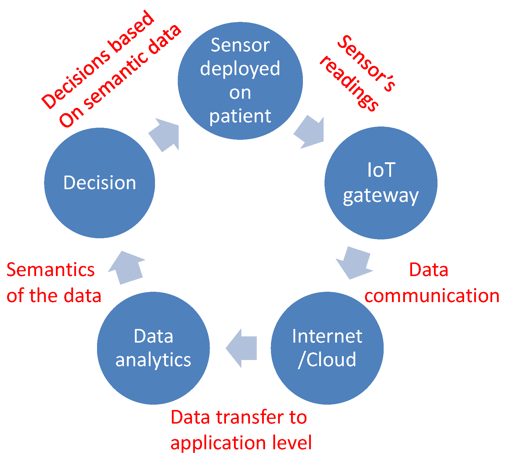
In FoG detection, the observations are generally the readings from the acceleration and motion sensors, which are mounted on the patient’s body [36]. Usually, the accelerometer is the preferred sensor for analyzing the gait of the subjects. In [37], a variety of parameters including measuring the intensity of physical activity and identifying the kind of movements are analyzed using a triaxial accelerometer on real-time systems. The IoT architecture for FoG detection is given in Figure 1. A 3D accelerometer sensor is used to collect the data, while the data analysis and storage are done on the cloud, which evaluates the severity of the situation. The system consists of two main parts: a smartphone (or a nearby computer), which provides an interactive environment to the subjects to configure the relevant settings, as well as serving as an IoT gateway and a cloud service for data-processing, since sensors are resource-constrained in general and do not have the capability of storing and processing data.

From the perspective of an IoT architecture, there are three layers that are involved in the sensing/actuation, processing and analyzing of data, being the sensing layer, network layer and application layer. At the bottom is the sensing and actuation layer, which senses data from the environment through sensors and smart objects. In IoT, these objects can be anything ranging from refrigerators to vehicles equipped with sensors. The next layer is the network layer, which fuses the data that come from the lower layer and transmit them to the Internet for further processing. Since smartphones act as the bridge between the sensors and cloud service, the network layer is comprised of smartphones. The final layer is the application layer, which provides data analytics and decision making through machine learning. The application layer is comprised of the cloud service. The results from data analytics are then relayed to wearable sensors and the actuators’ layer through the smartphones. Moreover, the subjects can use the smartphones to view their own performance based on processed results from the cloud; each smartphone houses a dedicated mobile app designed specifically for this purpose.

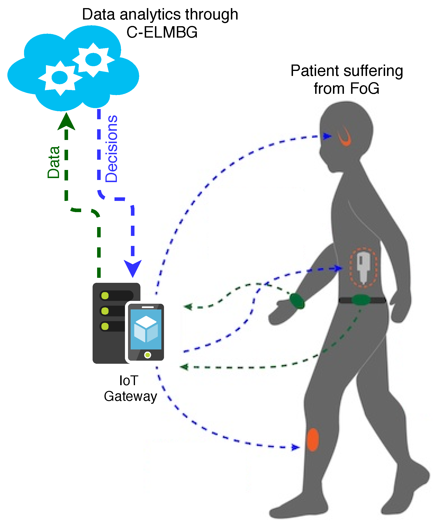
A scheme of online FoG detection through body-mounted sensors on a patient is shown in Figure 2. Motion patterns of the patient are analyzed using acceleration features of various sensors (NTMotion:AccGyro sensors [38]) mounted on the body. Since these sensors have very limited energy, the use of efficient low-power communication protocols is accentuated. Most appropriate candidates for communication include the Bluetooth protocol (802.15.1), Bluetooth low energy (BLE), ZigBee (802.15.4) and Wireless Body Area Network (802.15.6). Each of these protocols has its own features and requirements; for example, BLE is specifically designed for short-range applications, which consume minimal power, such as health monitoring, while ZigBee provides communication in a personal operating space (POS) of 10 m [39]. Data from these sensors is collected at the smartphone, preferably using the BLE device due to its better energy efficiency as compared to ZigBee and other protocols [40], which then transmits the data to the cloud.

Today’s infrastructure of IoT consists of various feasible options to transmit the data from smartphones to the cloud such as backhaul WiFi networks or cellular data networks (e.g., long-term evolution (LTE)) [41]. The rationale behind the use of the cloud service is that it offers several advantages such as accessibility and scalability on demand, which means that rather than patients always carrying an expensive piece of hardware to process complex data, this job can be outsourced to the cloud. Furthermore, the cloud can store the patient’s historic data en masse, which can also provide insight into patient’s health and also help in online training of the machine learning algorithms. The machine learning algorithms are the core of the whole system, which can recognize any pattern hidden within the recorded data, account for any correlation between different observations and also provide long-term benefits of medical diagnostics. Through these algorithms, earlier diagnosis of the disease is possible, and it can also help in reducing the costs by allowing one to circumvent expensive lab test. Another important aspect is the continual maturity of the machine learning algorithms, which are now part of the many software packages such as Python and MATLAB. Clouds can also provide better diagnostic information using visualization of the data. In fact, visualization is helpful for physicians to interpret the connection between different observations and respond accordingly. Visualizing is an effective way to represent data in a human-readable format and to make some meaningful analysis out of it. The cloud performs data analytics and provides feedback and decisions to the smartphone, which relays it to the sensor/actuator layer. In the event of FoG detection, the patients receive a feedback (decision). Finally, gait rehabilitation is initiated in the form of auditory and vibration signals.

3. Constrained Optimization-Based Extreme Learning Machine with Bagging

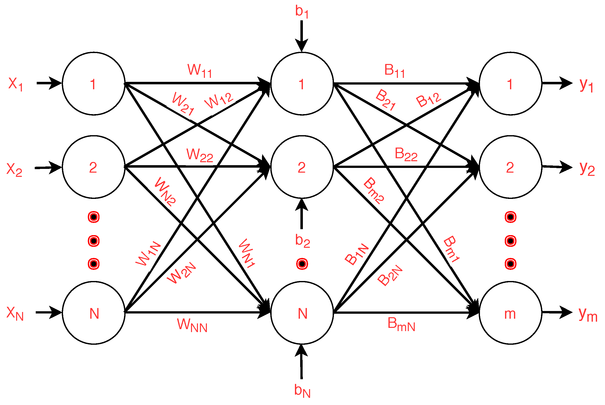
Bootstrap aggregating or bagging is an ensemble method used to improve the stability and accuracy of a machine learning algorithm for the classification problem. The idea of bagging is to generate n new training datasets from a given training set of size N by sampling and replacing. Based on the n generated bootstrap samples, n individual classifiers are constructed to predict the output of the test data. C-ELM is considered to be the base learner for the bagging method. The sampled training datasets are trained with the base classifier to generate the prediction output. The number of weak learners (P), where each weak learner contributes to the better accuracy of the final predicted model, needs to be evaluated and provided as an input to the bagging model. This is because bagging helps in reducing variability in the predictions. The final decision of a classification model that uses bagging is made by applying majority voting. The structure of the base classifier (C-ELM) for bagging is given in Figure 3.

As shown in Figure 3, C-ELM is categorized into three sub-layers. These sub-layers are generally known as the output (m output nodes), hidden (N hidden nodes or neurons) and input (N input nodes) layer. Nodes of the input and hidden layers are fully connected by some input weights $w_i={[w_{i1},w_{i2},...,w_{iN}]}^T$, where $i=1,2,...,\overline{N}$. On the other hand, nodes of the hidden and output layers are fully connected by another set of weights, which is given by $B_j={(B_{j1},B_{j2},...,B_{j\overline{N}})}^T$, where $j=1,2,...,m$. For any input observation vector $\mathbf{x}={(x_1,x_2,...,x_N)}^T$, the hidden layer matrix $\mathbf{H}$ can be calculated as $\mathbf{H}=g(w_i^{T}x+b_i)$, where g(.) denotes the kernel/activation function and $b_i$ gives the bias of the i-th neuron. The final predicted vector $\overline{y}={(\overline{y_1},\overline{y_2},...,\overline{y_m})}^T$ is given by:

$$\overline{y}=\sum _{i=1}^{\overline{N}}{B}_{ji}\mathbf{H}$$

(1)

ELM owes its popularity to the fact that the input weights and the biases do not need to be trained. The same logic is followed by C-ELM, as well, where $w_i$ and $b_i$, $i=1,2,...,\overline{N}$ are taken randomly.

The goal of C-ELM is to learn the output weights $B_j$ based on a set of training instances. Therefore, given a training set $S=\left[(x_k,y_k)\right|x_k\in R^k,y_k\in R^m,k=[1,2,...,K]]$, where $x_k=[x_{k1},x_{k2},...,x_{kK}]$ and $y_k=[y_{k1},y_{k2},...,y_{kK}]$ are respectively the input and the target output vectors of a particular training instance k. To learn the output weights $B_j$ from the training dataset, the following objective function needs to be solved:

Minimize $L(\vartheta ,\zeta )=\frac{1}{2}\parallel {\vartheta }^2\parallel +\frac{C}{2}{\sum }_{k=1}^K\parallel {{\zeta }_k}^2\parallel$ subject to the constraints:

$${\vartheta }^{T}h\left(X_k\right)=y_k-{\zeta }_k$$

where ${\zeta }_k$ is the predicted error of the k instances, C is a parameter for regularization, ${\vartheta }_{\overline{N}\times m}=[B_1,B_2,...,B_m]$ and matrix $h\left(X_k\right)$ of size $\overline{N}\times 1$ is given as follows,

$$h\left(X_k\right)=\left[\begin{array}{c}g(w_1^T{x}_k+b_1)\\ g(w_2^T{x}_k+b_2)\\ .\\ .\\ g(w_{\overline{N}}^T{x}_k+b_N)\end{array}\right]$$

(2)

In order to solve the constraint given as above, we now apply the Kuhn–Tucker conditions (Lagrange multipliers) [42]; the solution thus obtained is:

$$\vartheta ={(\frac{I_{\overline{N}\times \overline{N}}}{C}+H^{T}H)}^{-1}{H}^{T}Y$$

(3)

where $I_{\overline{N}\times \overline{N}}$ represents an identity matrix of size $\overline{N}\times \overline{N}$. The matrix H can now be represented as:

$$H=\left[\begin{array}{c}h{\left(x_1\right)}^T\\ h{\left(x_2\right)}^T\\ .\\ .\\ h{\left(x_K\right)}^T\end{array}\right],Y=\left[\begin{array}{c}{y}_1^T\\ y_2^T\\ .\\ .\\ y_K^T\end{array}\right]$$

(4)

For any instance k, the target output vector $y_k$ can be defined as:

$$y_{kj}=\left\{\begin{array}{cc}1:\hfill & \mathrm{when}\mathrm{instance}k\mathrm{belongs}\mathrm{to}\mathrm{category}j\hfill \\ -1:\hfill & \mathrm{when}\mathrm{instance}k\mathrm{does}\mathrm{not}\mathrm{belong}\mathrm{to}\mathrm{category}j\hfill \end{array}\right.$$

(5)

where $1\le j\le m$ and m is the total number of categories present in the dataset. For an input vector $x_k$, if ${\overline{y}}_k$ is the predicted vector, then the category of $x_k$ is:

$$x_k=arg\underset{j\in 1,2,..,m}{max}\left({\overline{y}}_{kj}\right)$$

(6)

The algorithm for C-ELMBG is presented in Algorithm 1. It is further divided into two phases, training and testing. First, we train the algorithm using the training dataset, and then, in the testing phase, we evaluate the algorithm using the test dataset. In the training phase, a specified random portion of the dataset is taken, the input weights (w) are assigned and the matrix (H) is calculated. The activation function that is considered for the analysis of the classifier using C-ELMBG is the sigmoid function [23]. The procedure for finding the number of hidden neurons is the same as [34]. Once the network has been trained, the testing samples (disjoint from the training samples) can be applied to it, in order to validate the accuracy of the developed network. The matrix $H_{test}$ is calculated using the test input weights $w_{test}$. Later, in order to make a final decision, the majority voting principle is leveraged. If the number of positive values of $\rho$ is greater than the number of negative values of $\rho$, then ${\psi }_{test}$ belongs to ‘freeze’ class; otherwise, it belongs to the ‘not freeze’ class.

Algorithm 1: C-ELM with bagging (C-ELMBG).

4. Experimental Analysis

4.1. Simulation Setup

The validity of the base classifier C-ELM and C-ELMBG is presented through experimental analysis on the Daphnet FoG dataset [43] using MATLAB R2016a. A detailed comparison of the results of our proposed scheme with the state-of-the-art statistical learning models like classification and regression trees (CART), linear discriminant analysis (LDA), SVM and random forests (RF) is also presented.

Description of the FoG Dataset

The Daphnet FoG dataset [43] was originally collected to come up with methods that can detect gait freeze in a person from the various wearable acceleration sensors placed on their legs and hips [7]. It was collected from 10 patients suffering from PD, who regularly experienced FoG in their routine life. The source of the data was 3D acceleration sensors, which were attached to each subject’s shank, thigh and trunk, and measurements were taken with a sampling frequency of 64 Hz, transmitted via a Bluetooth device to the system, also attached to the subjects. Each subject underwent two sessions of data recording, where each session lasted for about 15 minutes and consisting of a number of steps including straight line walking, walking with numerous turns and more realistic activities like fetching coffee, opening doors, etc. In total, there are nine features available in the dataset including three-dimensional accelerations of ankle, shank and trunk. A detailed description of these features and the output is also presented in

Table 2. Description of the features.

Sr. No.	Features	Description
1.	Ankle acceleration	horizontal forward acceleration (mg)
2.	Ankle acceleration	vertical acceleration (mg)
3.	Ankle acceleration	horizontal lateral acceleration (mg)
4.	Upper leg acceleration	horizontal forward acceleration (mg)
5.	Upper leg acceleration	vertical acceleration (mg)
6.	Upper leg acceleration	horizontal lateral acceleration (mg)
7.	Trunk acceleration	horizontal forward acceleration (mg)
8.	Trunk acceleration	vertical acceleration (mg)
9.	Trunk acceleration	horizontal lateral acceleration (mg)
10.	Annotation	1–> no freeze 2–> freeze

.

The starting point of FoG was taken as the point when the regular gait pattern was arrested, while the ending point was the resumption of regular gait (i.e., left-right steps). The results of the experiments were divided into three classes: 1, no freeze; 2, freeze; and 0, those data that were not part of the experiment. For experimental purposes in this work, only Classes 1 and 2 have been considered. To successfully apply C-ELM and C-ELMBG, the datasets with the result as Class 2 belong to the output Category +1, and those with the result as Class 1 belong to the output Category −1. The experimental analysis is performed on two sets of data, which have been chosen randomly. The first dataset contains 20,410 samples, while the second dataset contains 27,392 samples chosen from the data of the different patients.

Firstly, the training set is applied on the model to fine-tune the weights of the network, and then, validation of the model is done using validation dataset. For the 20,410 and the 27,392 samples considered, 9382 samples have been randomly taken for testing, thus creating the validation set, and the rest of the 11,028 and the 18,010 samples respectively have been used for training purposes, thus creating two individual training datasets. The details of the dataset are given in

Table 3. Description of the dataset and confusion matrix.

(a) Dataset Description
	Classification		Total
	Freeze	Not Freeze
Test dataset	5120	4262	9382
Training dataset 1	2907	8121	11,028
Training dataset 2	12,145	5865	18,010
(b) Confusion Matrix
		Predicted
		Yes	No
Actual	Yes	True positive ($T_p$)	False negative ($F_n$)
	No	False positive ($F_p$)	True negative ($T_n$)

a.

4.2. Simulation Results

The performance of the developed classifier is calculated using the confusion matrix as given in Table 3b. False negative ($F_n$) is also known as miss rate, false positive ($F_p$) as fall-out, true negative ($T_n$) as specificity and true positive ($T_p$) as hit rate, sensitivity and recall. In a confusion matrix, the term $T_p$ refers to the cases in which the classifier predicted a ‘yes’ and the patient actually suffered from FoG. For the $T_n$ cases, the classifier gives a negative answer, and the person actually did not exhibit FoG conditions. On the contrary, for the $F_p$, the classifier predicts a patient to have manifested FoG, but the patient actually did not. For the $F_n$ cases, the reverse is true.

4.2.1. Metrics for Evaluation of a Classifier

Some metrics can be derived from a confusion matrix to evaluate a classifier. These metrics can be expressed as follows:

To determine how often a classifier gives correct predictions, its accuracy can be evaluated as:

$$\phi =\frac{T_p+T_n}{T_n+F_p+F_n+T_p}$$

(7)

where $\phi$ is accuracy, $T_p$ is true positive, $T_n$ is true negative, $F_p$ is false positive and $F_n$ is false negative. The balanced F-score, also known as the F1 score ($F_1$), can also be used to measure the accuracy of a classifier. It is formulated as:

$$F_1=\frac{2\times T_p}{2\times T_p+F_p+F_n}$$

(8)

The sensitivity ($\rho$) or recall of a classifier indicates its capacity to correctly predict the number of positives in a dataset and can be given as:

$$\rho =\frac{T_p}{T_p+F_n}$$

(9)

Specificity ($\varsigma$) is the proportion of negatives in a binary classification test that are correctly identified.

$$\varsigma =\frac{T_n}{T_n+F_p}$$

(10)

Matthews’ correlation coefficient (MCC) is used in machine learning to determine the predictive quality of a binary classification. It gives a correlation between the observed and the predicted binary classification.

$$\Theta =\frac{(T_p\times T_n)-(F_p\times F_n)}{\sqrt{(T_p+F_p)\times (T_p+F_n)\times (T_n+F_p)\times (T_n+F_n)}}$$

(11)

where $\Theta$ is the MCC.

4.2.2. Parameter Settings

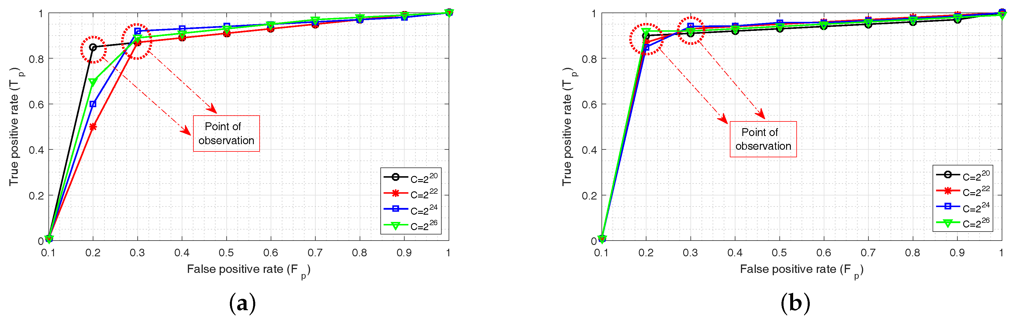
The parameter settings for the successful implementation of C-ELM are described next. In (3), the regularization parameter C needs to be evaluated. This value is chosen during the training period and remains unchanged during the testing phase. Figure 4a,b shows the receiver operating characteristic (ROC) curves for the test set used in Training Set 1 and Training Set 2, respectively for different values of $C$. The C values for the four curves are $C=2^{20},C=2^{22},C=2^{24}$ and $C=2^{26}$. The curve corresponding to $C=2^{24}$ has the highest area under curve (AUC) among all the curves; its value being equal to $0.8994$, pertaining to Training Set 1, and $0.9248$ for Training Set 2. The other AUC values in Figure 4a are $0.8631,0.8734$ and $0.8781$, and those in Figure 4b are $0.9142,0.9016$ and $0.8979$, respectively for $C=2^{20},C=2^{22}$ and $C=2^{26}$. Thus, $C=2^{24}$ has been considered as the regularization parameter value for both C-ELM and C-ELMBG. The point of observation in the graphs provides the point where a sudden change is detected. For example, in Figure 4a at $F_p=0.3$ and onwards, the values of $T_p$ gets smoother for $C=2^{22}$, $C=2^{24}$ and $C=2^{26}$, and at $F_p=0.2$ and onwards, the value of $T_p$ for $C=2^{20}$ gets smoother. The same is the case with Figure 4b, as well.

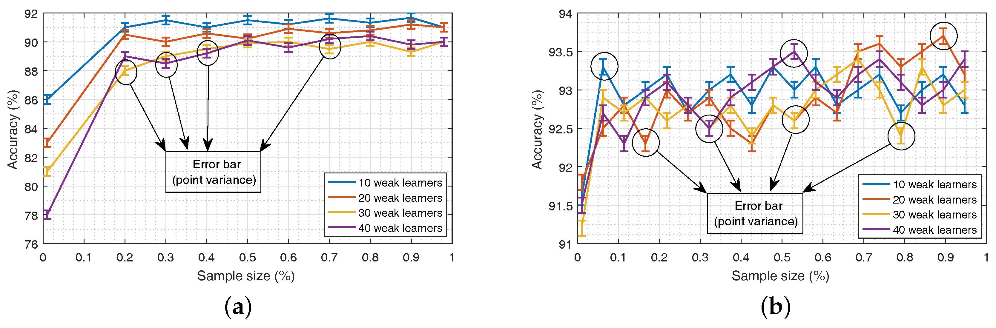
For C-ELMBG, the parameters that need to be considered are the number of weak learners P and the sampling rate. With Training Dataset 1, the best accuracy of the test set is achieved with the 10 weak learners and the sample size of 70%, as shown in Figure 5a. On the other hand, with Training Dataset 2, the classifier gives the best accuracy with the 20 weak learners when the sampling size is 90%, as shown in Figure 5b. The error bars in the graphs provide the variability of error or uncertainty in the reported data samples. This error can be calculated by $\frac{{\sum }_{i=1}^R{({\phi }_i-\overline{\phi })}^2}{R-1}$. This gives the standard deviation (point variance) of the reported sample data, which is then divided by the square root of the number of sample measurements (R) to yield uncertainty. Here, R gives the number of runs for each sampling rate and is taken to be 30. The value of initial hidden nodes is taken as 20.

4.2.3. Comparison with Other Classifiers

Table 4. Results of the test set.

(a) Training Set 1
	LDA	CART	C-ELM	C-ELMBG	RF	SVM
$T_p$	3298	4106	4704	4802	4559	0
$T_n$	4112	3675	3746	3815	3713	4263
$F_p$	151	587	517	447	549	0
$F_n$	1821	1014	415	318	561	5119
$\phi$ (%)	78.98	82.94	90.12	91.87	88.17	45.43
$\rho$ (%)	64.42	80.21	91.89	93.79	89.05	0
$\varsigma$ (%)	96.46	86.22	87.99	89.51	87.10	100
$F_1$	0.7968	0.8368	0.9103	0.9262	0.8914	NaN
$\Theta$	0.6287	0.6615	0.8005	0.8354	0.7614	NaN
AUROC	0.8044	0.8322	0.8994	0.9165	0.8806	0.5
(b) Training Set 2
	LDA	CART	C-ELM	C-ELMBG	RF	SVM
$T_p$	2948	4898	5087	5119	5120	5119
$T_n$	4154	3147	3648	3697	3157	0
$F_p$	108	1115	614	566	1105	4263
$F_n$	2172	221	33	0	0	0
$\phi$ (%)	75.7	85.76	93.11	93.97	88.23	54.57
$\rho$ (%)	57.58	95.68	99.37	100	100	100
$\varsigma$ (%)	97.47	73.83	85.59	86.73	74.08	0
$F_1$	0.7212	0.88	0.9402	0.9476	0.9026	0.706
$\Theta$	0.5849	0.7215	0.8663	0.8873	0.7806	NaN
AUROC	0.7753	0.8476	0.9248	0.9336	0.8704	0.5

a,b gives the values for the different metrics for C-ELM, C-ELMBG, LDA, CART, SVM and RF for Training Sets 1 and 2, respectively as given in Table 3a.

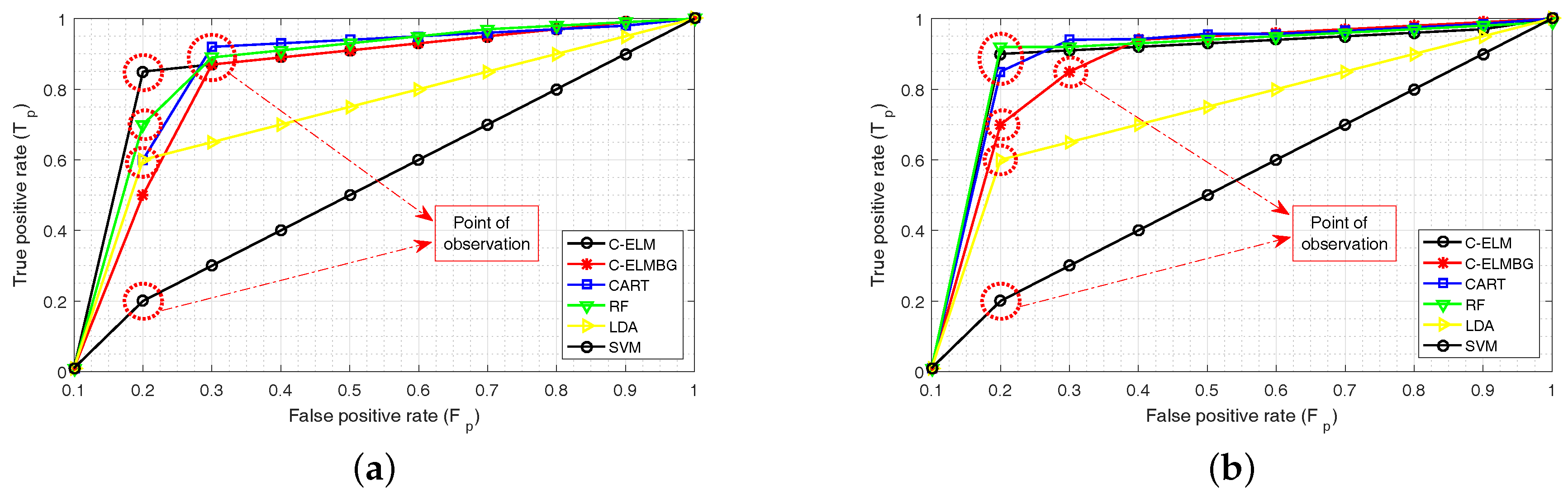
For the test dataset, C-ELM with bagging provides the best accuracy for both the training datasets. The F1-score is yet another parameter in binary classification to test the accuracy of the given classifier. The F1-score values for C-ELM and C-ELMBG show that they perform better than the other classifiers. RF performs better than the other three models, which can be attributed to its ensemble learning method that uses bagging. However, both F1-score and accuracy cannot capture the true essence of a classifier, as they do not comprehend the size of the four classes of the confusion matrix (Table 3b). This is where MCC comes to the rescue, which evaluates the proportion of each class of the confusion matrix. The MCC values show that C-ELMBG has the best performance among all the classification techniques while taking both training sets into account. Similarly in terms of sensitivity, C-ELM and C-ELMBG score better than other algorithms. Though SVM has a specificity value of 100%, its sensitivity value is zero for the results in Table 4a, making it practically improbable. Similarly, the sensitivity value of SVM in Table 4b is 100%, but its specificity value is zero, thus further confirming its impracticality. Here, again, LDA has a better specificity value in Table 4b than other classifiers. Hence, it is difficult to conclude which classifier renders the best performance. Thus, to confirm the prognostication ability of a classifier, the area under a receiver operating characteristic curve (AUROC) is taken into consideration. AUROC provides the summary statistics for the goodness of a classifier in a binary classification task, thus resolving the ambiguity regarding the performance of a classifier. Figure 6a,b shows the ROC curves for each of the classifiers over all possible thresholds. Each of the curves are plotted for the $T_p$ rate against the $F_p$ rate. We can see from these figures that the performance of the C-ELMBG is lower as compared to other machine learning algorithms for smaller $F_p$ values, but as the value of $F_p$ increases, it bypasses the other algorithms in performance. The discussion on the point of observation is the same as discussed above for Figure 4a,b with the replacement of the regularization parameter with different machine learning algorithms.

From the results of AUROC from Table 4a,b, it can be concluded that the classifiers using C-ELM and C-ELMBG perform competitively better when compared to other state-of-the-art classifiers. In terms of AUROC, for the results in Table 4a using Training Dataset 1, C-ELM shows an accuracy improvement of 1.95% over RF, 7.18% over CART, 11.14% over LDA and 44.69% over SVM; whereas, the accuracy by using C-ELMBG is further improved by 3.7% over RF, 8.93% over CART, 12.89% over LDA and 46.44% over SVM. Moreover, for the results in Table 4b for Training Dataset 2, C-ELM shows an accuracy improvement of 4.88% over RF, 7.35% over CART, 17.41% over LDA and 54.57% over SVM; whereas, the accuracy by using C-ELMBG is further improved by 5.74% over RF, 8.21% over CART, 18.27% over LDA and 55.43% over SVM.

5. Conclusions

This paper adopts an extreme learning machine-based technique called C-ELM to act as a base classifier for C-ELMBG, which is an ensemble model to detect FoG in a patient using data from the body-mounted acceleration sensors placed on his/her legs and hips. A model based on C-ELMBG classifies a new observation as either freeze or no-freeze based on the value of the predicted vector. Through experimental analysis based on the two training sets, it can be seen that C-ELMBG achieves an accuracy as high as almost 94% (93.97%). The overall performances of the base classifier CELM and C-ELMBG are also reflected through their values of AUROC. A comparative study with the existing state-of-the-art machine learning techniques such as LDA, CART, SVM and RF also shows the superiority of C-ELM and C-ELMBG. C-ELM and C-ELMBG can be easily implemented using an IoT-based system to successfully detect FoG in a patient suffering from PD.

References

- Handte, M.; Foell, S.; Wagner, S.; Kortuem, G.; Marrón, P.J. An internet-of-things enabled connected navigation system for urban bus riders. IEEE Internet Things J. 2016, 3, 735–744. [Google Scholar] [CrossRef]
- Xu, G.; Yu, W.; Griffith, D.; Golmie, N.; Moulema, P. Toward integrating distributed energy resources and storage devices in smart grid. IEEE Internet Things J. 2017, 4, 192–204. [Google Scholar] [CrossRef] [PubMed]
- Yu, T.; Wang, X.; Shami, A. Recursive principal component analysis-based data outlier detection and sensor data aggregation in IoT systems. IEEE Internet Things J. 2017, 4, 2207–2216. [Google Scholar] [CrossRef]
- Pringsheim, T.; Jette, N.; Frolkis, A.; Steeves, T.D. The prevalence of Parkinson’s disease: A systematic review and meta-analysis. Mov. Disord. 2014, 29, 1583–1590. [Google Scholar] [CrossRef] [PubMed]
- Islam, S.R.; Kwak, D.; Kabir, M.H.; Hossain, M.; Kwak, K.S. The internet of things for health care: A comprehensive survey. IEEE Access 2015, 3, 678–708. [Google Scholar] [CrossRef]
- Bloem, B.R.; Hausdorff, J.M.; Visser, J.E.; Giladi, N. Falls and freezing of gait in Parkinson’s disease: A review of two interconnected, episodic phenomena. Mov. Disord. 2004, 19, 871–884. [Google Scholar] [CrossRef] [PubMed]
- Bachlin, M.; Plotnik, M.; Roggen, D.; Maidan, I.; Hausdorff, J.M.; Giladi, N.; Troster, G. Wearable assistant for Parkinson’s disease patients with the freezing of gait symptom. IEEE Trans. Inf. Technol. Biomed. 2010, 14, 436–446. [Google Scholar] [CrossRef] [PubMed]
- Mazilu, S.; Hardegger, M.; Zhu, Z.; Roggen, D.; Troster, G.; Plotnik, M.; Hausdorff, J.M. Online detection of freezing of gait with smartphones and machine learning techniques. In Proceedings of the 6th IEEE International Conference on Pervasive Computing Technologies for Healthcare (PervasiveHealth), San Diego, CA, USA, 21–24 May 2012; pp. 123–130. [Google Scholar]
- Kubota, K.J.; Chen, J.A.; Little, M.A. Machine learning for large-scale wearable sensor data in Parkinson’s disease: Concepts, promises, pitfalls, and futures. Mov. Disord. 2016, 31, 1314–1326. [Google Scholar] [CrossRef] [PubMed]
- Pepa, L.; Ciabattoni, L.; Verdini, F.; Capecci, M.; Ceravolo, M. Smartphone based fuzzy logic freezing of gait detection in parkinson’s disease. In Proceedings of the IEEE/ASME 10th International Conference on Mechatronic and Embedded Systems and Applications (MESA), Senigallia, Italy, 10–12 September 2014; pp. 1–6. [Google Scholar]
- Rodriguez-Martin, D.; Sama, A.; Perez-Lopez, C.; Catala, A.; Arostegui, J.M.M.; Cabestany, J.; Bayes, A.; Alcaine, S.; Mestre, B.; Prats, A.; et al. Home detection of freezing of gait using support vector machines through a single waist-worn triaxial accelerometer. PLoS ONE 2017, 12, e0171764. [Google Scholar] [CrossRef] [PubMed]
- Lawrence, S.; Giles, C.L.; Tsoi, A.C.; Back, A.D. Face recognition: A convolutional neural-network approach. IEEE Trans. Neural Netw. 1997, 8, 98–113. [Google Scholar] [CrossRef] [PubMed]
- Kalchbrenner, N.; Grefenstette, E.; Blunsom, P. A convolutional neural network for modelling sentences. arXiv, 2014; arXiv:1404.2188. [Google Scholar]
- Liu, F.; Zhong, D. GSOS-ELM: An RFID-Based Indoor Localization System Using GSO Method and Semi-Supervised Online Sequential ELM. Sensors 2018, 18, 1995–2010. [Google Scholar] [CrossRef] [PubMed]
- Krizhevsky, A.; Sutskever, I.; Hinton, G.E. Imagenet classification with deep convolutional neural networks. In Proceedings of the 25th International Conference on Neural Information Processing Systems, Lake Tahoe, Nevada, 3–5 December 2012; pp. 1097–1105. [Google Scholar]
- Uzair, M.; Shafait, F.; Ghanem, B.; Mian, A. Representation learning with deep extreme learning machines for efficient image set classification. Neural Comput. Appl. 2018, 30, 1211–1223. [Google Scholar] [CrossRef]
- Camps, J.; Sama, A.; Martin, M.; Rodriguez-Martin, D.; Perez-Lopez, C.; Alcaine, S.; Mestre, B.; Prats, A.; Crespo, M.C.; Cabestany, J.; et al. Deep Learning for Detecting Freezing of Gait Episodes in Parkinson’s Disease Based on Accelerometers. In International Work-Conference on Artificial Neural Networks; Springer: Cham, Switzerland, 2017; pp. 344–355. [Google Scholar]
- Hagan, M.T.; Demuth, H.B.; Beale, M.H.; De Jesús, O. Neural Network Design; PWS Pub.: Boston, MA, USA, 1996; Volume 20. [Google Scholar]
- Huang, G.B.; Zhu, Q.Y.; Siew, C.K. Extreme learning machine: Theory and applications. Neurocomputing 2006, 70, 489–501. [Google Scholar] [CrossRef] [Green Version]
- Wong, C.M.; Vong, C.M.; Wong, P.K.; Cao, J. Kernel-based multilayer extreme learning machines for representation learning. IEEE Trans. Neural Netw. Learn. Syst. 2018, 29, 757–762. [Google Scholar] [CrossRef] [PubMed]
- Han, F.; Huang, D.S. Improved extreme learning machine for function approximation by encoding a priori information. Neurocomputing 2006, 69, 2369–2373. [Google Scholar] [CrossRef]
- Rong, H.J.; Huang, G.B.; Sundararajan, N.; Saratchandran, P. Online sequential fuzzy extreme learning machine for function approximation and classification problems. IEEE Trans. Syst. Man Cybern. Part B Cybern. 2009, 39, 1067–1072. [Google Scholar] [CrossRef] [PubMed]
- Rumelhart, D.E.; McClelland, J.L. Parallel Distributed Processing: Explorations in the Microstructure of Cognition; Foundations; MIT Press: Cambridge, MA, USA, 1986; Volume 1. [Google Scholar]
- Zhu, Y.; Liang, J.; Chen, J.; Ming, Z. An improved NSGA-III algorithm for feature selection used in intrusion detection. Knowl. Based Syst. 2017, 116, 74–85. [Google Scholar] [CrossRef]
- Huang, G.B.; Zhu, Q.Y.; Mao, K.; Siew, C.K.; Saratchandran, P.; Sundararajan, N. Can threshold networks be trained directly? IEEE Trans. Circ. Syst. II Express Briefs 2006, 53, 187–191. [Google Scholar] [CrossRef]
- Huang, G.B.; Ding, X.; Zhou, H. Optimization method based extreme learning machine for classification. Neurocomputing 2010, 74, 155–163. [Google Scholar] [CrossRef]
- Huang, G.B.; Zhou, H.; Ding, X.; Zhang, R. Extreme learning machine for regression and multiclass classification. IEEE Trans. Syst. Man Cybern. Part B Cybern. 2012, 42, 513–529. [Google Scholar] [CrossRef] [PubMed]
- Cortes, C.; Vapnik, V. Support-vector networks. Mach. Learn. 1995, 20, 273–297. [Google Scholar] [CrossRef] [Green Version]
- Wang, R.; Kwong, S.; Wang, D.D. An analysis of ELM approximate error based on random weight matrix. Int. J. Uncertain. Fuzziness Knowl. Based Syst. 2013, 21, 1–12. [Google Scholar] [CrossRef]
- Huang, G.B.; Chen, L.; Siew, C.K. Universal approximation using incremental constructive feedforward networks with random hidden nodes. IEEE Trans. Neural Netw. 2006, 17, 879–892. [Google Scholar] [CrossRef] [PubMed]
- Ma, C.; Ouyang, J.; Chen, H.L.; Zhao, X.H. An efficient diagnosis system for Parkinson’s disease using kernel-based extreme learning machine with subtractive clustering features weighting approach. Comput. Math. Methods Med. 2014, 2014, 985789. [Google Scholar] [CrossRef] [PubMed]
- Chen, H.L.; Wang, G.; Ma, C.; Cai, Z.N.; Liu, W.B.; Wang, S.J. An efficient hybrid kernel extreme learning machine approach for early diagnoses of Parkinson’s disease. Neurocomputing 2016, 184, 131–144. [Google Scholar] [CrossRef]
- Huang, G.B.; Chen, L. Enhanced random search based incremental extreme learning machine. Neurocomputing 2008, 71, 3460–3468. [Google Scholar] [CrossRef] [Green Version]
- Feng, G.; Huang, G.B.; Lin, Q.; Gay, R.K.L. Error minimized extreme learning machine with growth of hidden nodes and incremental learning. IEEE Trans. Neural Netw. 2009, 20, 1352–1357. [Google Scholar] [CrossRef] [PubMed]
- Wong, S.Y.; Yap, K.S.; Yap, H.J. A Constrained Optimization based Extreme Learning Machine for noisy data regression. Neurocomputing 2016, 171, 1431–1443. [Google Scholar] [CrossRef]
- Tao, W.; Liu, T.; Zheng, R.; Feng, H. Gait analysis using wearable sensors. Sensors 2012, 12, 2255–2283. [Google Scholar] [CrossRef] [PubMed]
- Mathie, M.J.; Coster, A.C.; Lovell, N.H.; Celler, B.G. Accelerometry: Providing an integrated, practical method for long-term, ambulatory monitoring of human movement. Physiol. Meas. 2004, 25, R1–R20. [Google Scholar] [CrossRef] [PubMed]
- Roggen, D.; Bächlin, M.; Schumm, J.; Holleczek, T.; Lombriser, C.; Tröster, G.; Widmer, L.; Majoe, D.; Gutknecht, J. An educational and research kit for activity and context recognition from on-body sensors. In Proceedings of the IEEE Internation Conference on Body Sensor Networks (BSN), Singapore, 7–9 June 2010; pp. 277–282. [Google Scholar]
- Pothuganti, K.; Chitneni, A. A comparative study of wireless protocols: Bluetooth, UWB, ZigBee, and Wi-Fi. Adv. Electron. Electr. Eng. 2014, 4, 655–662. [Google Scholar]
- Siekkinen, M.; Hiienkari, M.; Nurminen, J.K.; Nieminen, J. How low energy is bluetooth low energy? comparative measurements with zigbee/802.15.4. In Proceedings of the IEEE Wireless Communications and Networking Conference Workshops (WCNCW), Paris, France, 1 April 2012; pp. 232–237. [Google Scholar]
- Soyata, T.; Ba, H.; Heinzelman, W.; Kwon, M.; Shi, J. Accelerating mobile-cloud computing: A survey. In Cloud Technology: Concepts, Methodologies, Tools, and Applications; IGI Global: Hershey, PA, USA, 2015; pp. 1933–1955. [Google Scholar]
- Kuhn, H.W.; Tucker, A.W. Nonlinear programming. In Traces and Emergence of Nonlinear Programming; Springer: Basel, Switzerland, 2014; pp. 247–258. [Google Scholar]
- Daphnet Freezing of Gait Dataset. Available online: https://archive.ics.uci.edu/ml/datasets/Daphnet+Freezing+of+Gait (accessed on 20 May 2018).
Figure 1.
Flow diagram for FoG detection with IoT.
Figure 2.
Online FoG detection through body-mounted sensors.
Figure 3.
C-ELM with N input nodes, N hidden nodes and m output nodes.
Figure 4.
Receiver operating characteristics (ROC) curves: (a) test set corresponding to Training Set 1 for different C values; (b) test set corresponding to Training Set 2 for different C values.
Figure 5.
Accuracy vs. sampling size for different numbers of weak learners: (a) bagging of test set for Training Set 1, (b) bagging of test set for Training set 2.
Figure 6.
Receiver operating characteristic (ROC) curves: (a) test set corresponding to Training Set 1 for different classifiers; (b) test set corresponding to Training Set 2 for different classifiers.