Focusing Schlieren Visualization of Transonic Turbine Tip-Leakage Flows †

1
Department of Mechanical Engineering, Muenster University of Applied Sciences, 48565 Steinfurt, Germany
2
Laboratory of Turbomachinery, Department of Power Engineering, Helmut-Schmidt University, 22043 Hamburg, Germany
*
Author to whom correspondence should be addressed.
†
This Paper is an Extended Version of Our Paper Published in the Proceedings of the 13th European Conference on Turbomachinery Fluid Dynamics and Thermodynamics, ETC13, Lausanne, Switzerland, 8–12 April 2019; Paper No. 326.
Int. J. Turbomach. Propuls. Power 2020, 5(1), 1; https://doi.org/10.3390/ijtpp5010001
Submission received: 23 September 2019
/
Revised: 18 December 2019
/
Accepted: 23 December 2019
/
Published: 2 January 2020
Abstract
:This paper presents a focusing schlieren system designed for the investigation of transonic turbine tip-leakage flows. In the first part, the functional principle and the design of the system are presented. Major design considerations and necessary trade-offs are discussed. The key optical properties, e.g., depth of focus, are verified by means of a simple bench test. In the second part, results of an idealized tip-clearance model as well as linear cascade tests at engine representative Reynolds and Mach numbers are presented and discussed. The focusing schlieren system, designed for minimum depth of focus, has been found to be well suited for the investigation of three-dimensional transonic flow fields in turbomachinery applications. The schlieren images show the origin and growth of the tip-leakage vortex on the blade suction side. A complex shock system was observed in the tip region, and the tip-leakage vortex was found to interact with the suction side part of the trailing edge shock system. The results indicate that transonic vortex shedding is suppressed in the tip region at an exit Mach number around = 0.8.
1. Introduction
Blade tip-leakage flows of unshrouded blade tips are known to reduce stage efficiency in axial flow turbines [1]. In incompressible flow, the loss associated with the tip-leakage flow typically accounts for one third of the overall loss of a turbine stage [2]. Additionally, tip-leakage flows can lead to enhanced heat transfer in the tip-clearance, reducing the turbine blade life in high-temperature gas turbines [3,4,5]. Consequently, a comprehensive body of literature exists on low speed tip-leakage flows. Far fewer studies available in the open literature have considered transonic and supersonic tip-leakage flows, as can be found in the final stages of low-pressure steam turbines, modern turbofan aero engines, and organic Rankine cycle (ORC) turbines. While some numerical studies on this topic exist [3,6,7], detailed experimental data are scarce.
Tip-leakage flows are known to be influenced by local flow details, leading to highly three-dimensional and rather complex flow structures. In compressible flows, e.g., transonic flows, the tip region is expected to be dominated by effects associated with supersonic flow, such as shock waves and expansion fans [4,8]. Traditionally, schlieren photography has been used in turbomachinery applications to investigate two-dimensional phenomena such as profile loss, or the wake flow and trailing-edge shock system of transonic blade profiles [9,10,11]. Conventional schlieren systems, e.g., z-type setups with parabolic mirrors, a point light source, and parallel beam of light, possess a practically infinite depth of focus (DOF) [12]. The final image formed by such a system contains all density gradients that occur along the optical axis, including flaws in wind tunnel windows and flow outside the test section. In addition, some weaker density gradients that occur in some part of the flow field, such as in the blade tip region, might not be visible at all, as they can be obscured by stronger phenomena from other parts of the flow field. For the analysis of transonic tip-leakage flows, it is therefore desirable to have a device available which allows to sharply focus on a specific plane, i.e., a focusing schlieren system.
In the following, a focusing schlieren system designed for the investigation of transonic turbine tip-leakage flows is presented. The paper is structured as follows: In the first part, the functional principle and design of the focusing schlieren setup are presented. Major design considerations and necessary trade-offs are discussed. In the second part, results of an idealized transonic tip-leakage flow and of full-scale linear cascade tests are presented and discussed briefly.
2. Literature Review
Schlieren photography is an experimental method used for visualizing density variations in transparent media. The schlieren method as it is known today was principally developed by Toepler [13] in the 19th century. Toepler was also the first to term the method “Schlieren”, which is the German word describing optical inhomogeneities in transparent media. Schlieren techniques utilize the fact that light slows down upon interacting with matter, causing a change in refractive index. For simple gases, such as air, the refractive index n is related to the local density via [12]
where k is the Gladstone–Dale constant. Optical inhomogeneities (e.g., caused by density variations in gas flows) refract the light rays in proportion to their gradients of refractive index. The ray deflection angles in x- and y-direction are described by [12]
Herein, x,y,z describe a right-handed Cartesian coordinate system. The schlieren system itself converts the ray deflection into a change in brightness. For further information on the theoretical background of the schlieren method the reader is referred to the excellent book by Settles [12].
The principle of focusing schlieren has been known for quite some time. However, compared to conventional schlieren setups, that are a standard tool in compressible flow research, focusing schlieren are much more uncommon. The idea of focusing schlieren was first described by Schardin [14] more than 70 years ago, but due to World War II he was not able to further pursue his idea. Based on Schardin’s work, two different versions of focusing schlieren systems emerged over the following years. Kantrowitz and Trimpi [15] designed a system that consisted of two wide-angle lenses but only allowed for a field of view smaller than the lens diameter. The other system was devised by Burton [16,17]. He only used a single lens and was the first to recognize that the field of view is only limited by the source grid size and not by the schlieren lens diameter.
The most recent developments to the method were made by Weinstein [18,19], who devised what has been termed in the literature as “the modern focusing schlieren system” [12]. Based on Schardin’s original system, he used a Fresnel lens to light the source grid and a high quality commercial camera lens as the schlieren lens. Thereby, he solved all problems that previous systems had suffered from, namely, a small field of view, a large DOF, and the difficulty of use [12]. The use of a Fresnel lens also increased the image brightness by a factor of approximately 100 [18].
Based on Weinstein’s focusing schlieren method, a number of studies utilizing focusing schlieren were carried out over the past two decades. Alvi et al. [20] added a fiber-optic sensor to the system that allowed for optical turbulence measurements in the plane of sharp focus. A similar system was used later on by Garg and Settles [21] for measurements in a turbulent boundary layer. Gartenberg et al. [22] used a focusing schlieren system for recording detailed pictures of high Reynolds number flows in a cryogenic wind tunnel. The system proved to be sensitive enough to detect flow features at Mach numbers as low as . Taghavi and Raman [23] visualized supersonic screeching jets by means of a phase-conditioned focusing schlieren system. An approach for obtaining quantitative density data from focusing schlieren photographs was proposed by Cook and Chokani [24]. Their approach was based on the model of a spread function to account for out of focus information, but noise and difficulties in specifying the focusing depth affected the accuracy of the method. VanDercreek et al. [25] used focusing schlieren and deflectometry to investigate second-mode instabilities in boundary layer flows at hypersonic free stream conditions. Measurements in density fluctuations compared very well to pressure measurements.
Recently, focusing schlieren systems were used for supersonic combustion research [26,27,28]. In steady-state combustion test facilities, large temperature gradients exist across the test section side windows causing a change in refractive index of the glass. This change caused by the thermal gradients is larger than those caused by shock waves and expansion fans [28]. In such cases, focusing schlieren systems present an opportunity to bypass and suppress the thermal distortions on the side windows.
3. Focusing Schlieren System
A focusing schlieren system consists of the same basic components as conventional schlieren, in the sense that there is a light source, an imaging lens, a cutoff, and an image screen. However, instead of using a single point or slit light source, a two-dimensional array of slit light sources is used (Figure 1). These multiple light sources image through a lens onto a grid, which acts as a cutoff [19]. Therefore, a focusing schlieren system can be seen as a number of conventional schlieren systems stacked horizontally above each other [12].
The optical axes of the individual schlieren systems are inclined at a small angle. The resulting individual schlieren images only form a sharp image, if the image plane is focused on a corresponding plane in the test area. This effect is shown schematically in Figure 1 using the example of a single source point. All other density gradients that occur outside of this plane are, to some extent, offset from each other and will be blurry [15]. This effect, which is similar to the focusing principle of a normal lens, lends the focusing schlieren system its main characteristic, i.e., its ability to sharply focus on a specific plane.
3.1. Optical Layout
Figure 2 shows the schematic layout of the focusing schlieren system with all major components. An LED array with a nominal electrical power of is used as an extended light source. The present system uses a commercial LED module (manufacturer: Seoul ZC series; type: chip on board (COB)). COB LED modules have been found to be ideal for focusing schlieren systems, due to the very narrow spacing of the individual LED chips in the array, which results in a very uniform image illumination. A Fresnel lens with a diameter of and a focal length of redirects the light towards the schlieren lens. Initial tests with cheap Fresnel lenses form an overhead projector resulted in a poor image quality. The final system used acrylic Fresnel lenses with aspherically-grooved contours, that can be obtained from most optics suppliers.
Next to the Fresnel lens is the source grid, which consists of alternating opaque and transparent lines, where every transparent slit represents an individual light source. The counterpart is the cutoff grid, which is the photographic negative of the source grid, scaled down by a factor . For the present system, the transparent lines in the cutoff grid had a height of and the opaque stripes had a height of . Various methods for manufacturing the grids can be found in the literature. Traditionally, the cutoff grid is produced by exposing photographic film mounted at the sharp focus of the source grid [12]. Cutoff grids produced in such a way reproduce all imperfections of the source grid, as well as imperfections caused by the optical components of the system. Therefore, they are an exact photographic negative of the source grid. However, photographically exposed grids tend to deteriorate over time due to various small thermal expansions and misalignments [12]. For high-quality results, a recently exposed grid is necessary, which makes this method rather time-consuming and expensive. In the present case, the grids were made from acrylic sheets on which the black grid lines were printed by means of screen printing. This technique was found to be capable of producing opaque lines with sufficiently sharp edges. The quality of the prints was high enough that both source and cutoff grid could be printed. After several measurement campaigns, spanning over the period of one year, the printed grids show no sign of deterioration. If at some point the ink starts to fade, resulting in lower system sensitivity, a fresh set of grids can be obtained easily.
The schlieren lens is a fast commercial camera lens (Samyang 85 mm F1.4 AS IF UMC Aspherical) with a focal length of and a maximum aperture of . A second Fresnel lens is positioned at the image plane, which redirects the light towards the camera. Theoretically, a camera can be placed directly in the image plane. However, depending on the properties of the schlieren system, the image magnification can be considerable, resulting in a small field-of-view. This effect is especially pronounced for systems where the DOF is minimized, as will be shown in the next section (cf. Equation (4)). In the present case, a Fresnel lens with a diameter of and focal length of was necessary to focus the image on the camera. A monochrome high-speed camera with a CMOS sensor and a maximum image resolution of pixels was used for time-resolved schlieren images. However, for long exposure times, a standard digital reflex camera was also found to work well.
The distances between the different components and the schlieren lens can be estimated by applying the thin lens approximation
where F is the focal length of the schlieren lens, L is the distance between source grid and schlieren lens, is the distance between schlieren lens and cutoff grid, l is the distance from the plane of focus to the schlieren lens, and is the distance from the schlieren lens to the cutoff grid. It should be pointed out that the values obtained from Equation (3) only serve as a starting point in setting up the system. Adjustments will have to be made during the alignment of the system to account for optical aberrations and geometric imperfections.
3.2. System Properties
The design of a focusing schlieren system involves a trade-off between the different system properties, such as sensitivity, DOF, maximum image resolution, and field-of-view. For this study, the minimization of the DOF was a priority while maintaining adequate sensitivity and field-of-view.
Two definitions for the depth of sharp focus of a focusing schlieren system exist in the literature. According to Weinstein [19], the depth of sharp focus is the depth at which the loss of resolution due to being out of focus exceeds the resolution of the optical system:
Herein, is the clear aperture of the schlieren lens. The parameter w is the resolution limit due to grid refraction effects, which is written as [19]
where is the wavelength of light, b is the distance between two opaque lines at the cutoff grid, and describes the image magnification. The second definition, the depth of unsharp focus, is the depth at which the loss of resolution due to being out of focus exceeds the size of some flow detail [19]:
Following [18], the characteristic size of the flow detail was chosen with .
As mentioned in the previous section, the focusing effect results from the blending of many individual images. The number of blended images that form the final image on the image plane is defined as [19]
Herein, n is the number of grid lines in the cutoff grid per unit dimension. Weinstein [19] recommends a value of for good results.
The sensitivity of a schlieren system describes the minimum detectable deflection angle caused by the density gradient, where the schlieren system converts the deflection angle into a change in image brightness. Assuming that the smallest change in brightness detectable by the system is of the sensitivity of the system, the sensitivity can be written as [18]
where a is the unobstructed source image height on the cutoff plane. The term accounts for the focusing capabilities of the system [29] and the constant results from converting from radian to arc-second. The value obtained from Equation (8) has to be minimized for a system with high sensitivity.
The aforementioned trade-off between the different system properties is shown in Figure 3. Two of the most important design parameters, i.e., depth of sharp focus () and sensitivity , have been considered. Two different situations that a researcher commonly faces when setting up a focusing schlieren system are considered in the following: In the first situation, an existing setup is to be used but the test section can be positioned freely between source grid and schlieren lens, i.e., l is variable but , , and are constant. This situation is shown in Figure 3a. However, often the available space for setting up the schlieren system is extremely limited and the geometric parameters, e.g., L, , l, and , can not be varied to a great extent. This is often the case when the schlieren system has to be set up around a wind tunnel test section. This second situation is considered in Figure 3b, where , , , , and have been kept constant and the grid parameters a and b were varied.
Figure 3a shows DOF and sensitivity versus distance of the plane of sharp focus, i.e., the test section, from the schlieren lens. The value represents the location of the schlieren lens. The source grid is located at . In order to minimize the DOF, the focus plane would have to be close to the source grid ( to 1). This in turn would lead to a large value for the smallest detectable deflection angle , i.e., a system with poor sensitivity. Positioning the plane of interest halfway between the schlieren lens and source grid results in a more sensitive system but at the same time yields a maximum DOF. The best compromise can be obtained by placing the test section close to the schlieren lens (). However, the choice of the distance l is restricted by the following optical and geometrical properties of the schlieren system and test section: The minimum distance between plane of focus and schlieren lens is determined by the width of the wind tunnel test section and the distance between the front of the schlieren lens to its principal plane. If the plane of focus is to coincide with the center-plane of the test section, the distance l can not be less than half of the test section width plus the distance between the front of the lens to its principal plane. Additionally, has to be greater than the focal length of the schlieren lens () as otherwise no real image can be obtained. This limit is indicated by the left hatched area in Figure 3a. Similar considerations lead to the maximum possible distance between schlieren lens and test section , as the test section can not be placed closer to the source grid than half of the test section width (right hatched area in Figure 3a).
Figure 3b shows the influence of the grid parameters on DOF and system sensitivity. A fine grid with a high number of grid lines is required for a high-sensitivity system. A low number of grid lines results in a large DOF and poor sensitivity. For grids with more than 60 grid lines, no further significant reduction in DOF can be obtained. A further increase in the number of grid lines only reduces the minimum detectable deflection angle and hence increases system sensitivity. The typical range of grid lines of most focusing schlieren systems is shown in Figure 3b and is of order 6 to 40 grid lines. This corresponds to an unobstructed source image height at the cutoff grid of to . While the sensitivity increases with the number of grid lines, focusing schlieren setups are usually less sensitive than well designed conventional schlieren systems. As shown in Table 1, typical focusing schlieren systems have a minimum detectable deflection angle of order , whereas conventional schlieren systems can easily detect deflection angles of [12].
Table 1 shows the computed system properties of the focusing schlieren system used in this study. Two slightly different versions are listed, one for the idealized model and one for the linear cascade tests. The distance between the plane of focus and the schlieren lens l had to be increased slightly for the linear cascade tests due to geometric constraints, i.e., width of the test section. Thereby, the depth-of-unsharp focus () increased slightly, while all other system parameters remained almost unaffected. A comparison with focusing schlieren systems from the literature ( Table 1) shows that all systems have similar properties. This can in part be attributed to the choice of the schlieren lens, which in all three cases has a focal length of .
3.3. Validation of DOF
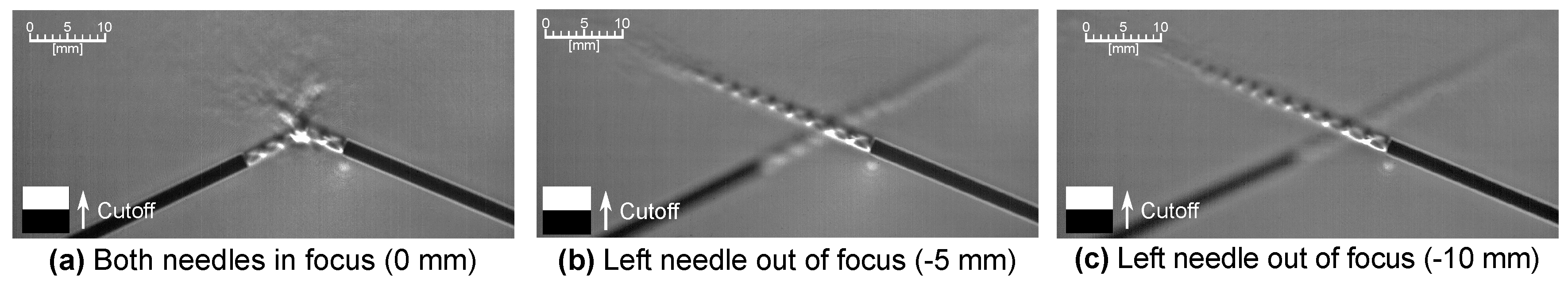
The calculated DOF was validated using a simple bench test. Results of this test are shown in Figure 4. Two hypodermic needles with an outer diameter of were placed in the plane of sharp focus. The needles were connected to the in-house compressed air supply, resulting in a pair of two crossed supersonic under-expanded jets. At first, both needles were placed in the plane of focus (cf. Figure 4a) and consequently, both supersonic jets appear equally sharp in the schlieren image. The left needle was then traversed along the optical axis, while the right needle remained in the plane of sharp focus. At an increment of mm (cf. Figure 4b), the jet is already unsharp and out of focus. At (cf. Figure 4c), only a shadow is visible in the background and no details of the flow structures can be made out. In total, images at ten different positions in increments of were taken. The detailed analysis showed that the effective DOF agrees with the computed value for given in Table 1.
The focusing effect can also be seen from the image intensity across the supersonic jet, shown in Figure 5. The image intensity I normalized by the average background intensity is plotted along a straight line segment of length three times the needle diameter d. The line is situated perpendicular to the needle center line at a distance of from the needle outlet, as shown schematically in Figure 5c. In Figure 5a, both needles are in sharp focus and the boundaries of the supersonic free-stream can be clearly seen as distinct peaks for both left and right needles. Upon moving the left needle out of focus, these peaks disappear in the corresponding intensity profile until the amplitude is comparable to the noise level of the image background (Figure 5c).
4. Application to Transonic Tip-Leakage Flows
Once the design parameters of the focusing schlieren system were tested and validated, the setup was used to investigate transonic tip-leakage flows. This section presents selected results of an idealized tip-clearance model as well as results of full scale linear turbine cascade tests. The main purpose of this section is to demonstrate the capabilities of the focusing schlieren system for the investigation of tip leakage flows. The results presented in the following were recorded with an exposure time of at a maximum frame rate of . Thereby, instantaneous flow structures could by captured in the individual images. During the tests, the schlieren system was focused on different planes along the blade span by traversing the entire schlieren system. The positioning accuracy of the traverse system was . The actual DOF relative to the channel height was for the idealized model and for the linear cascade.
4.1. Idealized Tip-Clearance Model
As a first test case, an idealized blade tip-clearance model (hereafter referred to as idealized model) was used to study fundamental tip-clearance effects at transonic conditions. The test section geometry is shown in Figure 6. A single blade, two passage cascade was used with a simplified blade profile that is representative of a steam turbine blade tip section. The test profile is similar to the tip sections investigated in [30] and consisted of straight line segments and circular arcs with tangential transitions. The test section side walls were contoured to obtain a realistic pressure distribution on the profile, similar to that of a real turbine blade with a stagger angle of . While this setup presents a simplification with respect to the situation in an actual turbine, or even a linear cascade, it has been shown in a previous investigation that it is a useful setup for the investigation of fundamental physical mechanisms [31]. Additionally, a similar concept was used recently by Melzer and Pullan [11] to study the role of vortex shedding in the trailing edge loss of transonic turbine blades.
The chord length of the blade profile in the idealized model was and the trailing edge diameter was chosen as , leading to a ratio of trailing edge diameter to geometrical throat of . The overall flow conditions can be characterized as follows: The inlet Mach number was of order and the isentropic blade exit Mach number was . This results in a Reynolds number based on chord length and exit Mach number of . Results for the idealized model were obtained at three different tip-clearance heights of , , and .
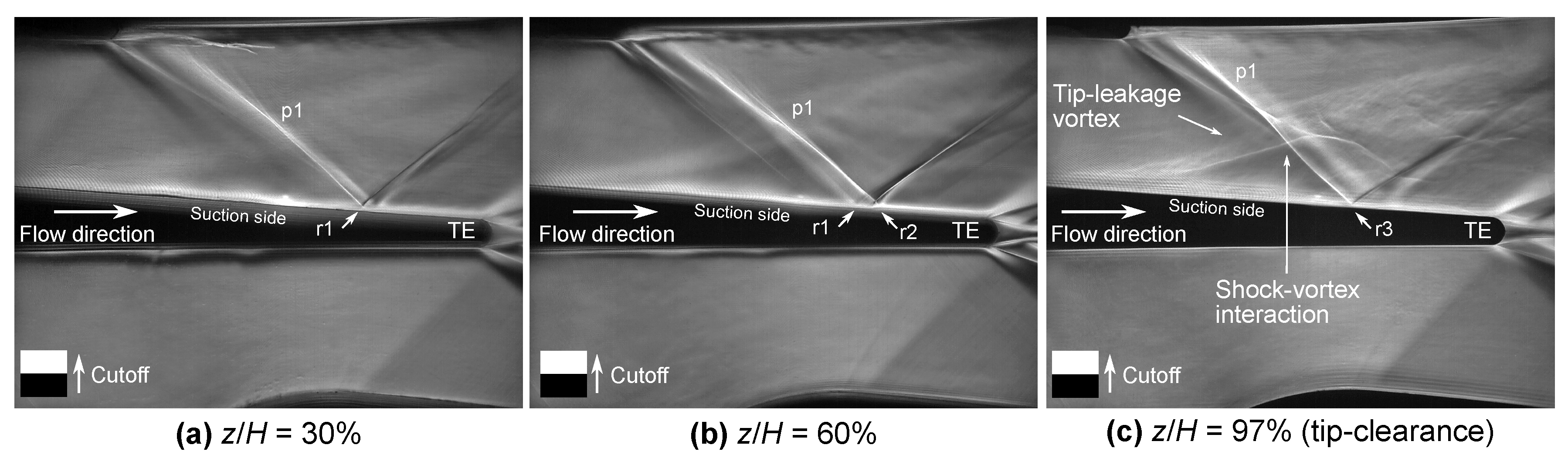
Figure 7 shows three images of the flow field for the idealized blade tip-clearance model, where the image section was chosen to show the rear two-thirds of the blade profile up to the trailing edge (TE) and the passage below and above the blade. The tip clearance for all images was . For each image, the schlieren system was focused on a different plane along the blade height. The position of the three different planes is shown in Figure 6b. A two dimensional flow field is observed close to the blade hub at (cf. Figure 7a). The pressure side TE shock (p1) of the neighboring blade profile (i.e., the profiled tunnel wall) impinges on the blade suction side and is reflected at point r1. The circular patterns or fringes visible close to the suction side surface are not a flow feature but artifacts of the Fresnel lens used in the image plane of the focusing schlieren system to relay the light towards the high-speed camera.
Slightly above midspan at (cf. Figure 7b), the pressure side TE shock (p1) of the neighboring blade profile is still clearly visible. The reflection point of the shock (r2) has shifted slightly further towards the TE with the old reflection point (r1) still visible but clearly out of focus. Additionally, a large flow structure can be seen schematically off the suction side surface. The structure is out of focus, but it can be made out that it originates downstream of the geometrical throat, coincident with the left image border of Figure 7b, and then grows in size as it moves further downstream along the blade suction side.
On closer examination of Figure 7c, this structure can be identified as the tip-leakage vortex. For Figure 7c, the focusing schlieren system was focused on the tip-clearance region at . The tip-leakage vortex (indicated by an arrow in Figure 7c) is now in sharp focus and dominates the flow field in the tip-clearance region. Additionally, an interaction between the TE edge shock p1 and the tip-leakage vortex can be observed, resulting in a reflection of p1 further upstream on the blade suction side at point r3.
The rear third of the blade chord length and the TE region are shown in Figure 8. Qualitatively, a similar behavior as described in the previous section can be observed. At (Figure 8a), the flow field is two-dimensional. The reflected TE shock from the neighboring blade (p1) is still visible at the left image border. At the trailing edge, the flow field is characterized by the trailing edge shocks on pressure and suction side (te1, te2) and the wake flow region further downstream. At and (Figure 8b,c), the turbulent fluctuations of the tip-leakage vortex become visible. Considering that the depth of unsharp focus of the schlieren system amounts to of the test section height H, the tip-leakage vortex is found to occupy approximately the upper third of the blade span. This observation is in agreement with oil-flow visualizations by Passmann et al. [31].
To further assess the capabilities of the focusing schlieren system for the investigation of transonic tip-leakage flows, different tip-clearance heights were considered. Figure 9 shows results for three tip-clearances of , , and . Four different planes of focus have been considered for each configuration. In the case of no tip-clearance (), the flow-field is two-dimensional (cf. Figure 9a–d). The flow field represents the well-known structure of supersonic trailing edge flow, as described in detail by Sieverding et al. [32], as well as Denton and Xu [33]. Dominant features are the triangular base region followed by the suction and pressure side trailing edge shock waves (te1, te2). Downstream of the base region, an unsteady blade wake is clearly visible in the schlieren images. No significant differences can be observed between the four different planes of focus, which was to be expected from a mostly two-dimensional flow field.
For a tip clearance of , the tip-leakage vortex becomes visible in the and focus planes (Figure 9g,h). In contrast, the flow field closer to midspan ( and ) is similar to the configuration without tip-clearance, although a systematic shift in the position of the shock reflection of shock p1 can be observed, as discussed earlier in this section.
Qualitatively, the same observations can be made for the largest tip-clearance of , shown in Figure 9i–l. The and focus planes show the two-dimensional flow field, which is mostly unaffected by the tip-leakage flow. For the tip-clearance, additional flow structures, indicated by the arrows 1 to 3, are observed in the vicinity of the tip-leakage vortex (cf. Figure 9k,l). At the same time, the suction side separation shock at the trailing edge and the trailing edge shock (te1) are out of focus in Figure 9l.
4.2. Transonic Turbine Cascade Tests
In addition to the tests on the idealized model, an investigation on a linear cascade with a representative turbine blade profile was undertaken. The experimental work for this part was carried out on the transonic cascade wind tunnel of the Laboratory of Turbomachinery at Helmut-Schmidt-University in Hamburg, Germany. A detailed description of the wind tunnel facility has been given by [34].
Figure 10 shows a sketch of the transonic cascade wind tunnel and the linear cascade test section. The blade profile used for this study was the well-known Von-Karman-Institute test profile VKI-1. The profile loss has been investigated independently by four institutions [10] and Wheeler et al. [3] conducted a numerical study on tip-leakage flow. The cascade consisted of seven blade profiles plus two boundary profiles to obtain periodic flow conditions around the central measurement blade, as shown in Figure 10. The profiles had a chord length of and were arranged at a stagger angle of . The blade spacing to chord ratio was , resulting in a spacing of . The cross-sectional area at the test section inlet was . The facility was operated under steady-state conditions and the total temperature at the cascade inlet was close to ambient. The turbulence intensity at the inlet was of order and was not increased artificially.
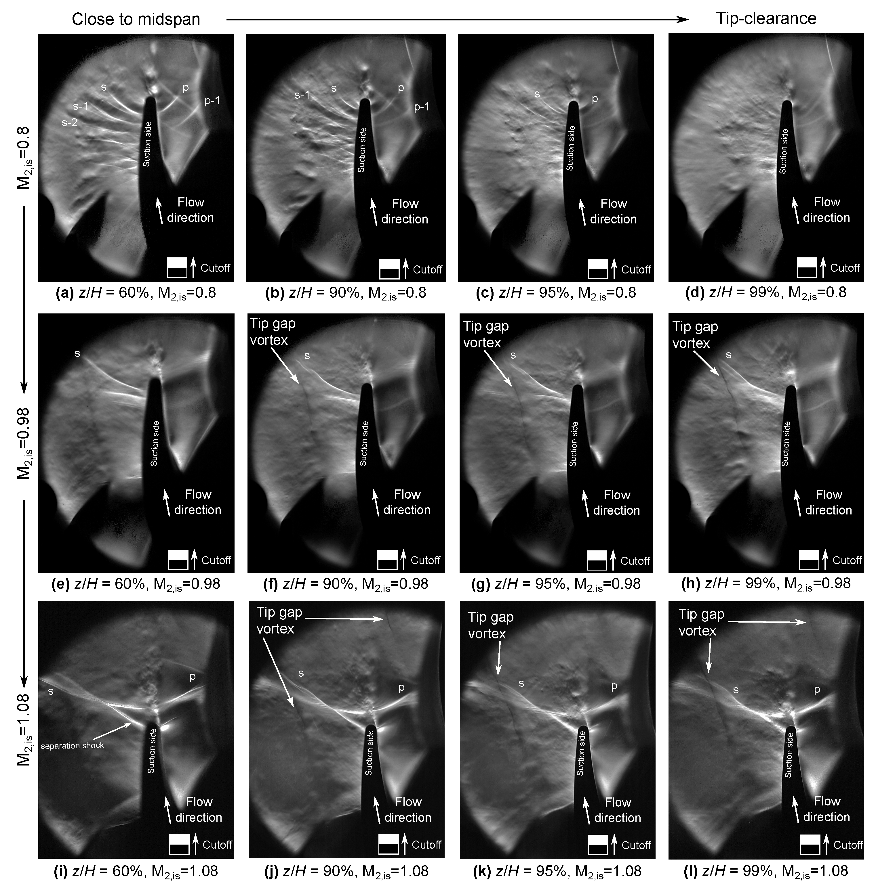
Figure 11 shows a set of results from the linear cascade tests. Three exit Mach numbers of , and were considered. For each Mach number, the schlieren system was focused on four different planes along the blade span, with the plane corresponding to the tip-clearance. All results were obtained at zero incidence and a tip-clearance of . At a blade exit Mach number of , transonic vortex shedding is observed at midspan (Figure 11a). Recently, Melzer and Pullan [11] investigated this phenomenon in detail and found that, depending on TE shape and size, transonic vortex shedding can occur at blade exit Mach numbers as low as . Under such conditions, shock waves can be shed with each shed vortex. This alternates on the pressure and suction side. The corresponding shocks are labeled with the letters p and s depending on their origin (cf. Figure 11a–c). While transonic vortex shedding is clearly visible at midspan, the tip-leakage flow seems to suppress this phenomenon. In the tip-clearance region (Figure 11d), only the turbulent fluctuations from the tip-leakage vortex are visible.
As the exit Mach number is increased to (Figure 11e–h), shock waves form close to the TE. Close to the blade tip (Figure 11g,h), evidence of the tip-leakage vortex becomes visible as a fine dark line. At present, it is not entirely clear what this line represents. However, based on the numerical results by Wheeler et al. [3] and the oilflow pattern of Passmann et al. [31] it is thought that this line represents the points where the tip-leakage flow separates from the cascade tip-wall and rolls up into the tip-leakage vortex. Finally, a pattern of oblique shock waves is formed at the trailing edge as the exit Mach number is increased to (Figure 11i–l). Close to midspan (Figure 11i), the suction side separation shock is visible that merges with the suction side TE shock (s).
The results presented in Figure 11 show that the focusing schlieren system is an adequate instrument for the investigation of transonic tip-leakage flows. The images show that the TE shock/wake system is influenced by the tip-leakage flow and, in the case of , suppresses transonic vortex shedding in the tip region.
5. Summary
A focusing schlieren system for the investigation of transonic tip-leakage flows was designed and commissioned. The system has a sharp DOF of and an unsharp DOF of . This was confirmed experimentally. Results of an experimental study on an idealized tip-clearance model and a transonic linear cascade were presented. These results represent the first focusing schlieren visualization of transonic tip-leakage flows and show that focusing schlieren is well-suited for the investigation of such phenomena. The results of the idealized model demonstrate the origin and spatial extent of the tip-leakage vortex and an interaction between tip-leakage vortex and oblique TE shock pattern was observed. The linear cascade results indicated that the shedding of shock waves caused by transonic vortex shedding at an exit Mach number of 0.8 was suppressed near the blade tip by the tip-leakage flow. At higher exit Mach numbers, the tip-leakage vortex formed a characteristic pattern which was interpreted to represent the separation area where the tip-leakage flow rolls up into a vortex.
Author Contributions
M.P. was responsible for the project administration, conceptualization, methodology, investigation, data curation, and original draft preparation. S.a.d.W. and F.J. were responsible for review and editing, supervision, and funding acquisition. All authors have read and agreed to the published version of the manuscript.
Funding
This research received no external funding. The APC of this paper is funded by Euroturbo.
Acknowledgments
The authors would like to thank Hendric Banholzer for his support during the design of the focusing schlieren system. Furthermore, the help of Marius Leetz, Janneck Harbeck, and Silvio Geist during the measurement campaign is highly acknowledged.
Conflicts of Interest
The authors declare no conflict of interest.
Nomenclature
| a | unobstructed source image height |
| A | clear aperture of schlieren lens |
| b | distance between cutoff grid lines |
| c | chord length |
| d | diameter |
| trailing edge diameter | |
| depth of sharp focus | |
| depth of unsharp focus | |
| depth of focus | |
| f-number of schlieren lens | |
| F | focal length of schlieren lens |
| g | pitch |
| H | channel height |
| I | image intensity value |
| average image background intensity value | |
| k | Gladstone–Dale constant |
| L | distance from source grid to schlieren lens |
| distance from schlieren lens to cutoff grid | |
| l | distance from schlieren object to schlieren lens |
| distance from schlieren lens to image plane | |
| m | magnification of image, |
| Mach number | |
| n | number of grid lines per millimeter at cutoff grid |
| p | pressure |
| angle change resulting in brightness change | |
| pairs of lines involved in forming each point in focusing schlieren image | |
| wavelength of light | |
| tip-clearance height |
References
- Dixon, S.L.; Hall, C. Fluid Mechanics and Thermodynamics of Turbomachinery, 7th ed.; Butterworth-Heinemann: Oxford, UK, 2013. [Google Scholar]
- Denton, J. Loss Mechanisms in Turbomachines. ASME J. Turbomach. 1993, 115, 621–656. [Google Scholar] [CrossRef]
- Wheeler, A.; Korakianitis, T.; Banneheke, S. Tip-Leakage Losses in Subsonic and Transonic Blade Rows. ASME J. Turbomach. 2013, 135, 011029. [Google Scholar] [CrossRef]
- Moore, J.; Elward, K. Shock Formation in Overexpanded Tip Leakage Flow. ASME J. Turbomach. 1993, 115, 392–399. [Google Scholar] [CrossRef]
- Jackson, A.; Wheeler, A.; Ainsworth, R. An Experimental and Computational Study of Tip Clearance Effects on a Transonic Turbine Stage. Int. J. Heat Fluid Fl. 2015, 56, 335–343. [Google Scholar] [CrossRef] [Green Version]
- Wheeler, A.; Sandberg, R. Numerical Investigation of the Flow Over a Model Transonic Turbine Blade Tip. J. Fluid Mech. 2016, 803, 119–143. [Google Scholar] [CrossRef] [Green Version]
- Dorney, D.; Griffin, L.; Huber, F. A Study of the Effects of Tip Clearance in a Supersonic Turbine. ASME J. Turbomach. 2000, 122, 674–683. [Google Scholar] [CrossRef]
- Wheeler, A.; Saleh, Z. Effect of Cooling Injection on Transonic Tip Flows. AIAA J. Propul. Power 2013, 29, 1374–1381. [Google Scholar] [CrossRef]
- Graham, C.; Kost, F. Shock Boundary Layer Interaction on High Turning Transonic Turbine Cascades. In Proceedings of the International Gas Turbine Conference and Exhibit and Solar Energy Conference, San Diego, CA, USA, 12–15 March 1979. [Google Scholar] [CrossRef]
- Kiock, R.; Lehthaus, F.; Baines, N.; Sieverding, C. The Transonic Flow Through a Plane Turbine Cascade as Measured in Four European Wind Tunnels. ASME J. Eng. Gas Turb. Power 1986, 108, 277–284. [Google Scholar] [CrossRef]
- Melzer, A.; Pullan, G. The Role of Vortex Shedding in the Trailing Edge Loss of Transonic Turbine Blades. ASME J. Turbomach. 2019, 141, 041001. [Google Scholar] [CrossRef] [Green Version]
- Settles, G. Schlieren and Shadowgraph Techniques: Visualizing Phenomena in Transparent Media; Springer Science Business Media: Berlin, Germany, 2012. [Google Scholar]
- Toepler, A. Beobachtungen Nach Einer Neuen Optischen Methode: Ein Beitrag zur Experimental-Physik; Max Cohen & Sohn: Bonn, Germany, 1864. [Google Scholar]
- Schardin, H. Die Schlierenverfahren und ihre Anwendungen. In Ergebnisse der Exakten Naturwissenschaften; Springer: Berlin, Germany, 1942; pp. 303–439. [Google Scholar]
- Kantrowitz, A.; Trimpi, R. A Sharp-Focusing Schlieren System. J. Aeronaut. Sci. 1950, 17, 311–314. [Google Scholar] [CrossRef]
- Burton, R. A Modified Schlieren Apparatus for Large Areas of Field. J. Opt. Soc. Am. 1949, 39, 907–908. [Google Scholar] [CrossRef] [PubMed]
- Burton, R. Notes on the Multiple Source Schlieren System. J. Opt. Soc. Am. 1951, 41, 858–859. [Google Scholar] [CrossRef]
- Weinstein, L. Large-Field High-Brightness Focusing Schlieren System. AIAA J. 1993, 31, 1250–1255. [Google Scholar] [CrossRef]
- Weinstein, L. Review and Update of Lens and Grid Schlieren and Motion Camera Schlieren. Eur. Phys. J. Spec. Top. 2010, 182, 65–95. [Google Scholar] [CrossRef]
- Alvi, F.; Settles, G.; Weinstein, L. A Sharp-Focusing Schlieren Optical Deflectometer. In Proceedings of the 31st Aerospace Sciences Meeting, Reno, NV, USA, 11–14 January 1993. [Google Scholar]
- Garg, S.; Settles, G. Measurements of a Supersonic Turbulent Boundary Layer by Focusing Schlieren Deflectometry. Exp. Fluids 1998, 25, 254–264. [Google Scholar] [CrossRef]
- Gartenberg, E.; Weinstein, L.; Lee, E. Aerodynamic Investigation With Focusing Schlieren in a Cryogenic Wind Tunnel. AIAA J. 1994, 32, 1242–1249. [Google Scholar] [CrossRef]
- Taghavi, R.; Raman, G. Visualization of Supersonic Screeching Jets Using a Phase Conditioned Focusing Schlieren System. Exp. Fluids 1996, 20, 472–475. [Google Scholar] [CrossRef]
- Cook, S.; Chokani, N. Quantitative Results From the Focusing Schlieren Technique. In Proceedings of the 31st Aerospace Sciences Meeting, Reno, NV, USA, 11–14 January 1993. [Google Scholar]
- VanDercreek, C.; Smith, M.; Yu, K. Focused Schlieren and Deflectometry at AEDC Hypervelocity Wind Tunnel No. 9. In Proceedings of the 27th AIAA Aerodynamic Measurement Technology and Ground Testing Conference, Chicago, IL, USA, 28 June–1 July 2010. [Google Scholar]
- Kouchi, T.; Goyne, C.; Rockwell, R.; McDaniel, J. Focusing-Schlieren Visualization in a Dual-Mode Scramjet. Exp. Fluids 2015, 56, 211. [Google Scholar] [CrossRef] [Green Version]
- Kouchi, T.; Masuya, G.; Yanase, S. Extracting Dominant Turbulent Structures in Supersonic Flow Using Two-Dimensional Fourier Transform. Exp. Fluids 2017, 58, 98. [Google Scholar] [CrossRef]
- Bühler, M.; Förster, F.; Dröske, N.; von Wolfersdorf, J.; Weigand, B. Design of a Focusing Schlieren Setup for Use in a Supersonic Combustion Chamber. In Proceedings of the 30th International Symposium on Shock Waves 2, Tel-Aviv, Israel, 19–24 July 2015; pp. 1467–1471. [Google Scholar] [CrossRef]
- Fish, R.; Parnham, K. Focusing Schlieren Systems; Report CP-54; Aeronautical Research Council: London, UK, 1950. [Google Scholar]
- Sieverding, C.; Decuypere, R.; Hautot, P. Investigation of Transonic Steam Turbine Tip Sections With Various Suction Side Blade Curvatures. In Proceedings of the Inst. of Mech. Engr. Design Conf. on Steam Turbines for the 1980’s, London, UK, October 1979; pp. 241–251. [Google Scholar]
- Passmann, M.; aus der Wiesche, S.; Joos, F. An Experimental and Numerical Study of Tip-Leakage Flows in an Idealized Turbine Tip Gap at High Mach Numbers. In Proceedings of the ASME Turbo Expo 2018: Turbomachinery Technical Conference and Exposition, Oslo, Norway, 11–15 June 2018. [Google Scholar]
- Sieverding, C.; Stanislas, M.; Snoeck, J. The Base Pressure Problem in Transonic Turbine Cascades. ASME J. Eng. Power 1980, 102, 711–718. [Google Scholar] [CrossRef]
- Denton, J.; Xu, L. The Trailing Edge Loss of Transonic Turbine Blades. ASME J. Turbomach. 1990, 112, 277–285. [Google Scholar] [CrossRef]
- Ober, B. Experimental Investigation on the Aerodynamic Performance of a Compressor Cascade in Droplet Laden Flow. Ph.D. Thesis, Helmut-Schmidt-Universität, Hamburg, Germany, 2013. [Google Scholar]
Figure 1.
Schematic illustration of the focusing effect of a focusing schlieren system using the example of a single source point (adapted from Weinstein [18]).
Figure 1.
Schematic illustration of the focusing effect of a focusing schlieren system using the example of a single source point (adapted from Weinstein [18]).

Figure 2.
Schematic layout of the focusing schlieren system with technical data of the main components.
Figure 2.
Schematic layout of the focusing schlieren system with technical data of the main components.

Figure 3.
Influence of design parameters on system properties. Depth of focus and sensitivity as function of (a) distance of plane of focus to schlieren lens and (b) number of grid lines.
Figure 3.
Influence of design parameters on system properties. Depth of focus and sensitivity as function of (a) distance of plane of focus to schlieren lens and (b) number of grid lines.
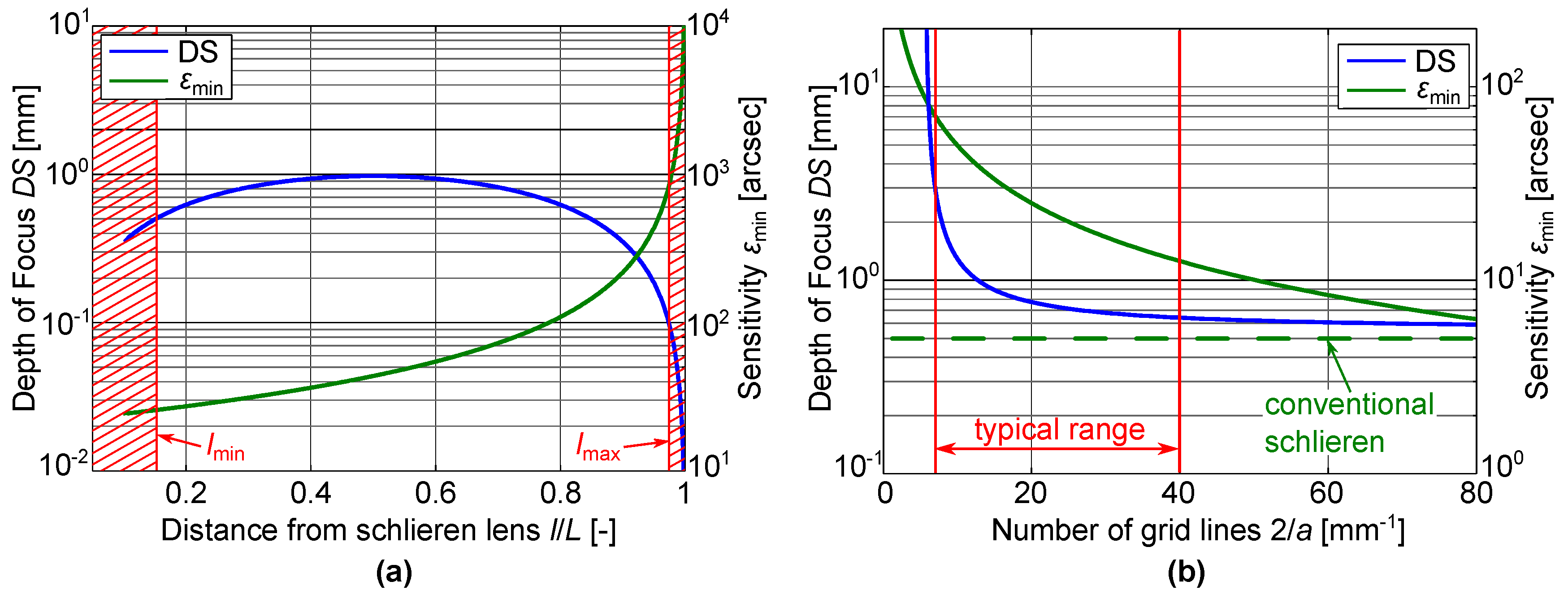
Figure 4.
Experimental validation of DOF by means of two crossed under-expanded jets. The outer diameter of the hypodermic needles was . The left needle was traversed along the optical axis (perpendicular to the image plane).
Figure 4.
Experimental validation of DOF by means of two crossed under-expanded jets. The outer diameter of the hypodermic needles was . The left needle was traversed along the optical axis (perpendicular to the image plane).

Figure 5.
Corrected image intensity in under-expanded jets from left and right needles for three planes of focus. (a) 0 mm; (b) mm; and (c) mm. The intensity profiles correspond to the photographs shown in Figure 4.
Figure 5.
Corrected image intensity in under-expanded jets from left and right needles for three planes of focus. (a) 0 mm; (b) mm; and (c) mm. The intensity profiles correspond to the photographs shown in Figure 4.

Figure 6.
Sketch of the test section geometry for the idealized blade tip-clearance model: (a) view of channel geometry in x-y-plane and (b) illustration of tip clearance and locations of focusing planes in x-z-plane.
Figure 6.
Sketch of the test section geometry for the idealized blade tip-clearance model: (a) view of channel geometry in x-y-plane and (b) illustration of tip clearance and locations of focusing planes in x-z-plane.
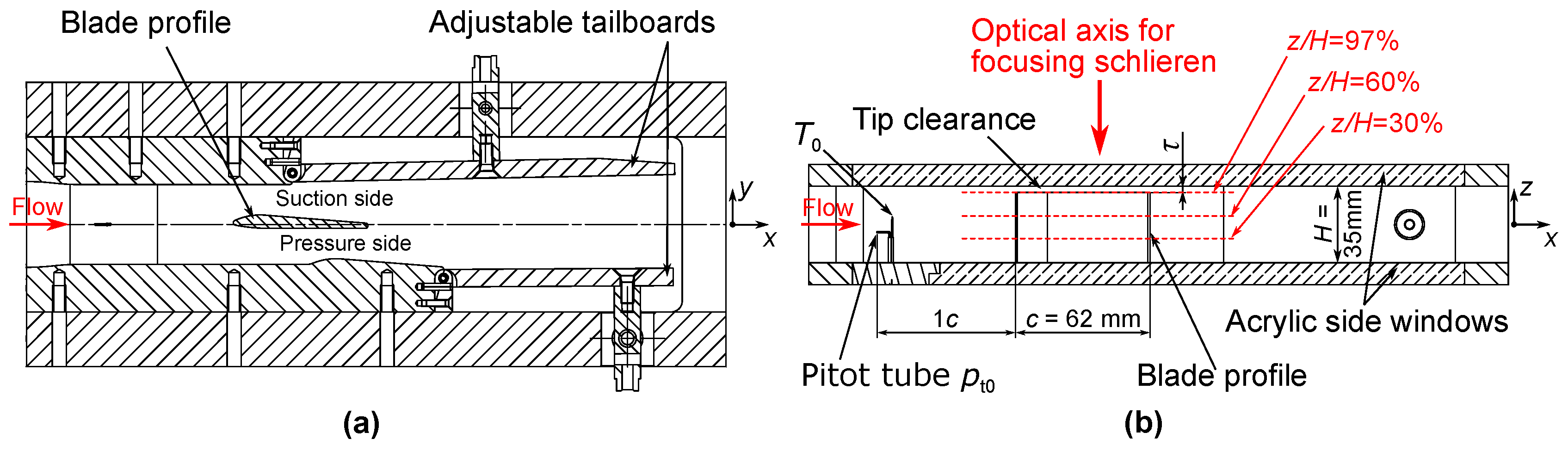
Figure 7.
Focusing schlieren images of the flow field in three different planes of focus for the idealized tip-clearance model. The tip-leakage vortex and its development along the chord length is shown for a tip-clearance of and .
Figure 7.
Focusing schlieren images of the flow field in three different planes of focus for the idealized tip-clearance model. The tip-leakage vortex and its development along the chord length is shown for a tip-clearance of and .

Figure 8.
Focusing schlieren images of the flow field in three different planes of focus for the idealized tip-clearance model. The rear third of the blade chord length and trailing edge region is shown for a tip-clearance of and .
Figure 8.
Focusing schlieren images of the flow field in three different planes of focus for the idealized tip-clearance model. The rear third of the blade chord length and trailing edge region is shown for a tip-clearance of and .

Figure 9.
Focusing schlieren images of the flow field in four different planes of focus. The rear third of the blade chord length and trailing edge region is shown for three tip-clearance heights of , images (a–d); , images (e–h); , images (i–l).
Figure 9.
Focusing schlieren images of the flow field in four different planes of focus. The rear third of the blade chord length and trailing edge region is shown for three tip-clearance heights of , images (a–d); , images (e–h); , images (i–l).
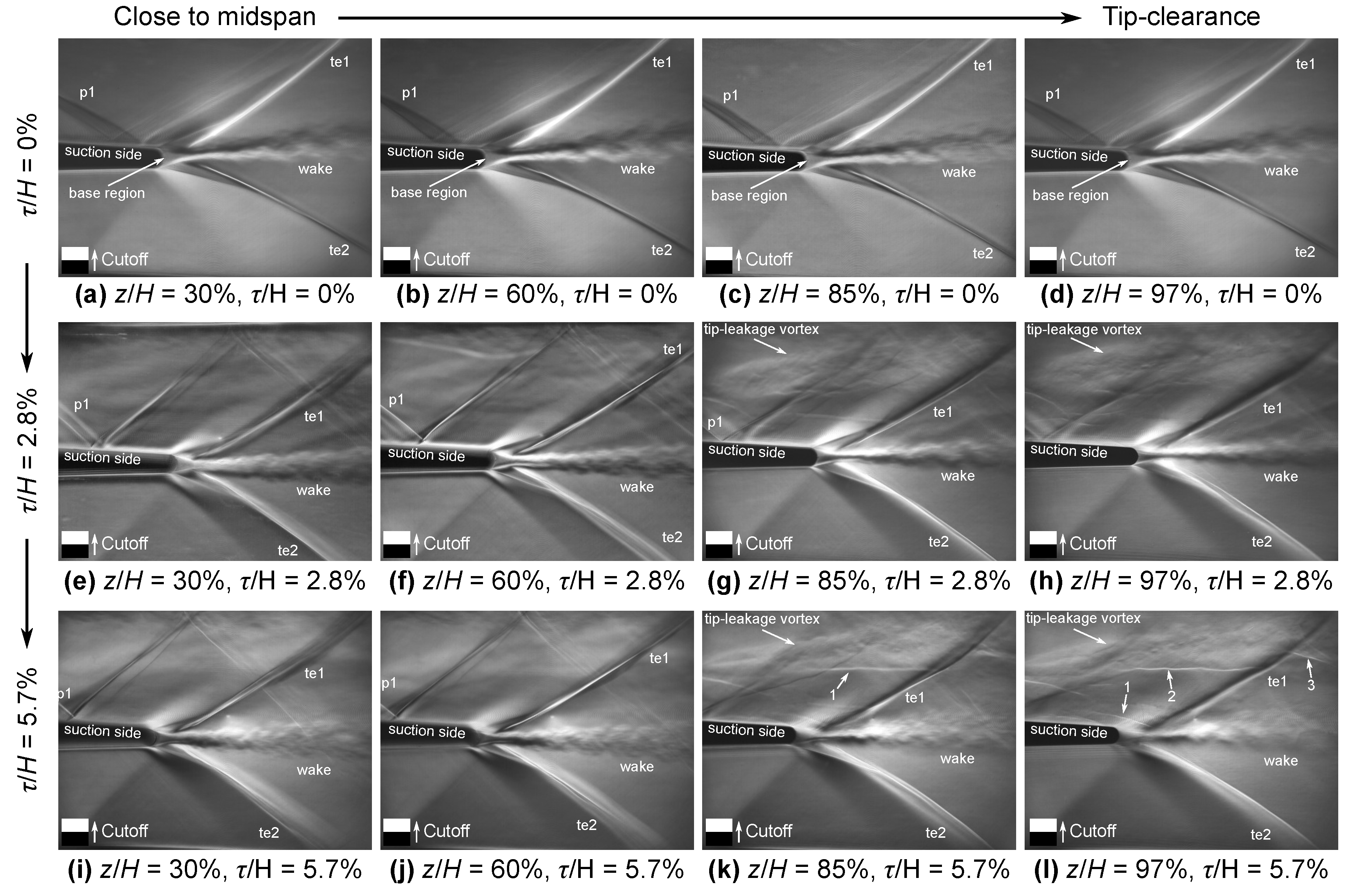
Figure 10.
Sketch of the transonic cascade wind tunnel with details of the linear cascade test section.
Figure 10.
Sketch of the transonic cascade wind tunnel with details of the linear cascade test section.
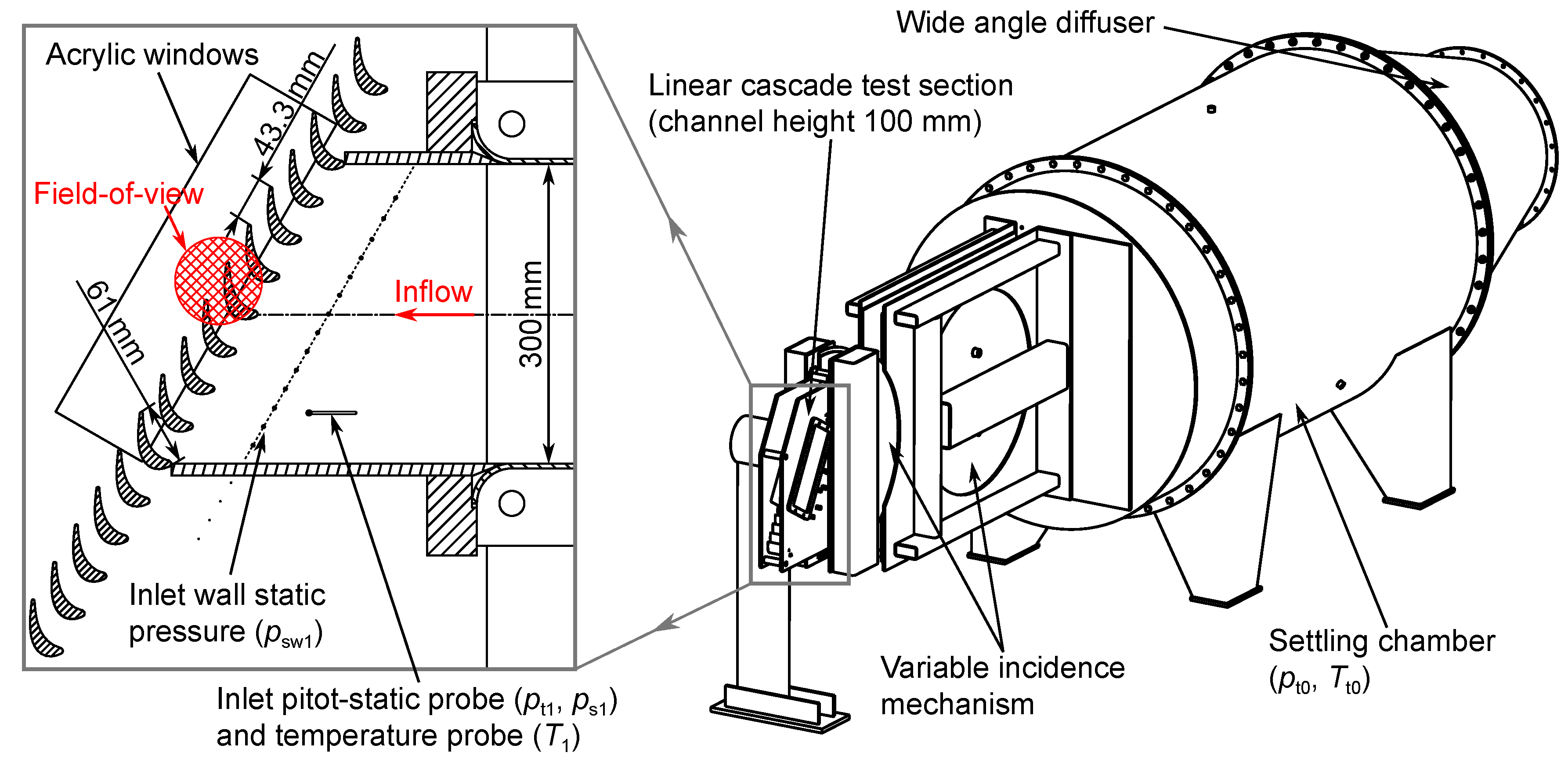
Figure 11.
Focusing schlieren images of the linear cascade test section for two mean exit Mach numbers of (a)–(d), (e)–(h), and (i)–(l) at incidence and a tip-clearance of . The field-of-view corresponds to the labeled area in Figure 10.
Figure 11.
Focusing schlieren images of the linear cascade test section for two mean exit Mach numbers of (a)–(d), (e)–(h), and (i)–(l) at incidence and a tip-clearance of . The field-of-view corresponds to the labeled area in Figure 10.

Table 1.
Specification of focusing schlieren system and comparison with systems from the literature.
Table 1.
Specification of focusing schlieren system and comparison with systems from the literature.
| L (mm) | (mm) | l (mm) | (mm) | (m) | (mm) | (mm) | (-) | (arcsec) | |
|---|---|---|---|---|---|---|---|---|---|
| Setup for idealized model tests | 850 | 94.5 | 110 | 374 | 100 | ±0.3 | ±3.6 | 24 | 25 |
| Setup for linear cascade tests | 850 | 94.5 | 120 | 291.5 | 100 | ±0.28 | ±3.9 | 26 | 25.4 |
| Kouchi et al. [26] | 640 | 98 | 110 | 374 | 70 | ±0.5 | ±3.6 | 36 | 17 |
| Bühler et al. [28] | 640 | 98 | 128 | 192 | - | - | ±4.2 | - | - |
© 2020 by the authors. Licensee MDPI, Basel, Switzerland. This article is an open access article distributed under the terms and conditions of the Creative Commons Attribution (CC BY) license (http://creativecommons.org/licenses/by/4.0/).
Share and Cite
MDPI and ACS Style
Passmann, M.; aus der Wiesche, S.; Joos, F. Focusing Schlieren Visualization of Transonic Turbine Tip-Leakage Flows. Int. J. Turbomach. Propuls. Power 2020, 5, 1. https://doi.org/10.3390/ijtpp5010001
AMA Style
Passmann M, aus der Wiesche S, Joos F. Focusing Schlieren Visualization of Transonic Turbine Tip-Leakage Flows. International Journal of Turbomachinery, Propulsion and Power. 2020; 5(1):1. https://doi.org/10.3390/ijtpp5010001
Chicago/Turabian StylePassmann, Maximilian, Stefan aus der Wiesche, and Franz Joos. 2020. "Focusing Schlieren Visualization of Transonic Turbine Tip-Leakage Flows" International Journal of Turbomachinery, Propulsion and Power 5, no. 1: 1. https://doi.org/10.3390/ijtpp5010001