Adjoint-Based Design Optimisation of an Internal Cooling Channel U-Bend for Minimised Pressure Losses ^†

Abstract

The success of shape optimisation depends significantly on the parametrisation of the shape. Ideally, it defines a very rich variation in shape, allows for rapid grid generation of high quality, and expresses the shape in a standard Computer Aided Design (CAD) representation. While most existing parametrisation methods fail at least one of these criteria, this work introduces a novel parametrisation method, which satisfies all three. A tri-variate B-spline volume is used to define the volume to be optimised. The position of the external control points are used as design parameters, while the internal control points are repositioned to ensure regularity of the transformation. The grid generation process transforms a Cartesian grid (defined in parametric space) to the physical space using the tri-variate net of control points. This process guarantees a high grid quality even for large deformations, and has extremely low computational cost as it only involves a transformation from parameter space to physical space. This allows the computation of the grid sensitivities with respect to the design variables at a fraction of the cost of a Computational Fluid Dynamics (CFD) iteration, therefore allowing the use of one-shot methods. This novel parametrisation is applied to the shape optimisation of a U-bend passage of a turbine-blade serpentine-cooling channel with the objective to minimise pressure losses. A steady state, Reynolds-Averaged, density-based Navier-Stokes solver is used to predict the pressure losses at a Reynolds number of 40,000. The sensitivities of the objective function with respect to the control points are computed using a hand-derived adjoint solver and geometry generation system. A one-shot approach is used to simultaneously converge flow, gradient and design, resulting in a rapid design approach with a design time equivalent to approximately 10 normal CFD runs, while still maintaining a CAD representation of the geometry. A large reduction in pressure loss is obtained, and the flow in the optimal geometry is analysed in detail.

1. Introduction

Internal cooling channels of modern gas turbine blades are a key enabler for high turbine inlet temperatures and hence higher efficiencies. Not only do they provide the air for film cooling, they simultaneously cool the internal structure as well. An effective scheme to cool down turbine blades with small coolant mass flow exists through multiple passages of the coolant by a serpentine layout of the internal cooling channel. A salient feature of such a scheme is the U-bend at the extremities of the straight passages, turning the flow 180 degrees. These bends are responsible for up to 25% of the total pressure losses of the internal cooling scheme, which reduces the overall cycle efficiency of the gas turbine plant. As a result, the study of U-bends has received profound attention in the literature.

Early literature studied the flow experimentally to better understand the flow physics. Examples include the work of Humphrey et al. [1], Chang et al. [2], Monson and Seegmiller [3], and Cheah et al. [4], to name a few. All contributions demonstrate the presence of secondary flow structures resulting from an imbalance between the centrifugal and pressure forces along the channel height. Furthermore, they all highlight the presence of a separation bubble near the internal wall in the second part of the bend, as a result of a strong adverse pressure gradient.

Another group of authors studied the numerical modelling of the turbulent flow. U-bends are indeed a challenging test case for turbulence models due to the presence of strong streamwise curvature and secondary flow motion. Recent studies by, e.g., Lucci et al. [5] and Schueler et al. [6] have demonstrated that eddy viscosity models can predict the flow reasonably well, as long as low-Reynolds formulations are used excluding the presence of wall functions (see Iacovides and Launder [7]). However, only second-order closure models can include the effect of streamline curvature on the turbulent structures, resulting in more accurate predictions as illustrated by Bonhof et al. [8] and Chen et al. [9]. Nevertheless, one and two-equation models are still the de facto standard in industrial design applications due to their reduced computational cost and higher robustness.

The final part of the literature is concerned with studies that seek to reduce the pressure losses of the U-bend. In the study of Liou and Chen [10] the divider wall thickness was increased, leading to a reduction in turbulence levels and a shortening of the reattachment length. The influence of the width of the passages, the corner radius and the clearance height was studied by Metzger et al. [11]. The addition of vanes in the bend to help guide the flow was studied by Bonhof et al. [12], leading to a significant reduction in pressure loss. Schueler et al. [13] confirm the reduction in pressure loss, but stress that improperly designed vanes can lead to severe deterioration of their performance.

The reduced pressure loss reported in the literature is obtained through a laborious approach that has been present ever since the invention of the wheel: modifications are tested and either accepted or rejected, after which new cycles of attempts follow. Engineers iterate from design to design, building up knowledge, but spending large amounts of time on testing and potentially exploring large numbers of uninteresting design alterations. This process can be automated to a large extend through the use of optimisation techniques. A recent example is the study of Zehner et al. [14], who optimised the divider wall of a sharp turn U-bend. They used an ice-formation technique to generate a starting profile of minimum energy dissipation, and further improved the performance by applying an evolutionary algorithm. Namgoong et al. [15] used Design of Experiments and a surrogate design space model for similar purposes. Verstraete et al. [16] used an evolutionary algorithm with a metamodel to reduce the large number of evaluations by Computational Fluid Dynamics (CFD). An experimental campaign presented in Colletti et al. [17] validates the proposed optimal shape. In a later study, Verstraete et al. [18] extended the scope to include heat transfer, which demonstrated that as long as the flow is separated, heat transfer and pressure loss are not necessarily conflicting objectives. For attached flows, however, a reduction in pressure loss can only be achieved at the expense of a reduced heat transfer by a reduction of the secondary flow.

The main shortcoming of the above-presented approaches is the limited degree of freedom that can be given to the shape. Indeed, to maintain a feasible degree of evaluations, evolutionary-based algorithms restrict the number of design shape variables to below 50. This limits the design to mainly 2D geometries extruded in the height direction. On the other hand, gradient-based methods do not exhibit this deterioration, and hence allow much richer design spaces, but this comes at the expense of computing the gradient. Additional problems include the need for efficient methods to deform the mesh from one iteration to another, as well as to maintain a link to the Computer Aided Design (CAD) model. Indeed, most adjoint methods modify a parametrised model of the mesh and need an additional step to reconstruct the CAD model of the optimal shape. This impairs optimality as geometrical details are invariably altered in such a process. Auriemma et al. [19] provided a solution to the problem by using a CAD-parametrised model of the U-bend; however, they faced issues with morphing the mesh to the modified CAD model.

In the present work we propose an alternative solution to the mesh deformation problem, while remaining closely linked to a CAD model. To this end, tri-variate B-splines will be employed, which defines a transformation from a 3-dimensional rectangular computational domain to the U-bend shape. This approach is similar to Gagnon et al. [20] and Martin et al. [21], where tri-variate B-splines are used to define the domain around external aerodynamic shapes. In their work the design space is controlled by a free-form deformation box placed around the tri-variate B-splines. In the present work, however, the control points of the tri-variate B-splines will be used directly as design parameters.

Through this approach, all faces of the U-bend shape remain B-spline surfaces, which allows a straight forward link to a watertight CAD model. The mesh generation is significantly simplified as it suffices to transform a structured rectangular mesh in the computational domain to 3D space, leading (as an additional benefit) to a very fast grid generation process. This allows the use of a one-shot method to speed up the convergence of the optimisation problem.

2. Methodology

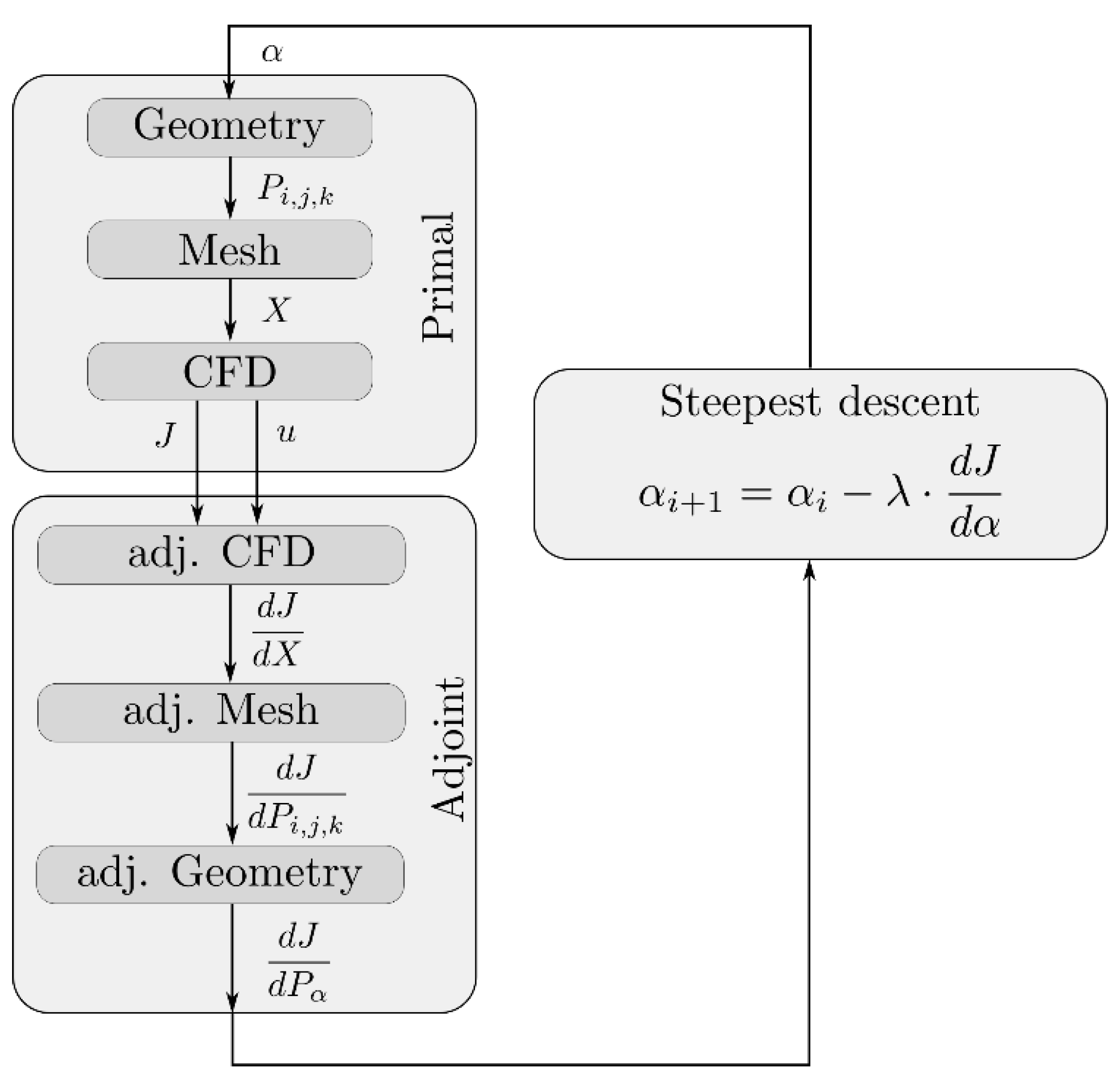
Figure 1 shows a schematic overview of the optimisation method. In the following sections the different components that constitute the algorithm will be discussed.

2.1. Geometry

The most commonly used approach to define a geometry in CAD is through a boundary representation (Brep) method, in which the skin of the geometry is defined analytically by surface patches which are stitched together. Although commercial CAD software packages such as CATIA or Solidworks give the user the impression of working with solid structures, in reality only the skin of the solid is being modelled. This is the most appropriate approach to model complex geometries, yet it has some drawbacks for use as a preprocessor to numerical simulations. Since the boundary representation only describes the skin, no direct link is defined to address internal points of the geometry, or more explicitly, there is no automatic transformation from a 3-dimensional computational domain to the internal volume of the geometry. This makes the grid generation process significantly more complex.

In the present work, we describe the geometry directly as a volume rather than a collection of surfaces. This is obtained through tri-variate B-splines, which are an extension of B-spline surfaces to volumes. Given a 3-dimensional array of control points P_i,j,k a tri-variate B-spline performs a mapping from the computational domain (u,v,w) to the 3-dimensional space (x,y,z) through:

$$\begin{array}{c}P\left(u,v,w\right)={\displaystyle {\displaystyle \sum }_{i=0}^{n_u}{\displaystyle \sum }_{j=0}^{n_v}{\displaystyle \sum }_{k=0}^{n_w}}{N}_i^{p_u}\left(u\right)·N_j^{p_v}\left(v\right)·N_k^{p_w}\left(w\right)·P_{i,j,k},\end{array}$$

(1)

with the number of control points n_u,n_v,n_w in the u,v,w directions respectively, the order of the basis functions (p_u,p_v,p_w) also in u,v,w directions, and the i-th basis function of order p $N_i^p$. For a non-decreasing set of knot vectors {u₀,u₁,…,u_m} the basis functions are recursively defined as:

$$N_i^0\left(u\right)=\{\begin{array}{cc}1& \hspace{1em}if u_i\le u\le u_{i+1}\\ 0& \hspace{1em}otherwise\end{array},$$

(2)

$$N_i^p\left(u\right)=\frac{u-u_i}{u_{i+p}-u_i}·N_i^{p-1}\left(u\right)+\frac{u_{i+p+1}-u}{u_{i+p+1}-u_{i+1}}·N_{i+1}^{p-1}\left(u\right).$$

(3)

The number of knots, e.g., m_u + 1 for the u-dimension, need to satisfy the following relation:

$$m=n+p+1,$$

(4)

while the first and last knot need to be repeated p + 1 times to assure a clamped B-spline, i.e., to ascertain that the corners of the tri-variate B-spline correspond to the corner control points.

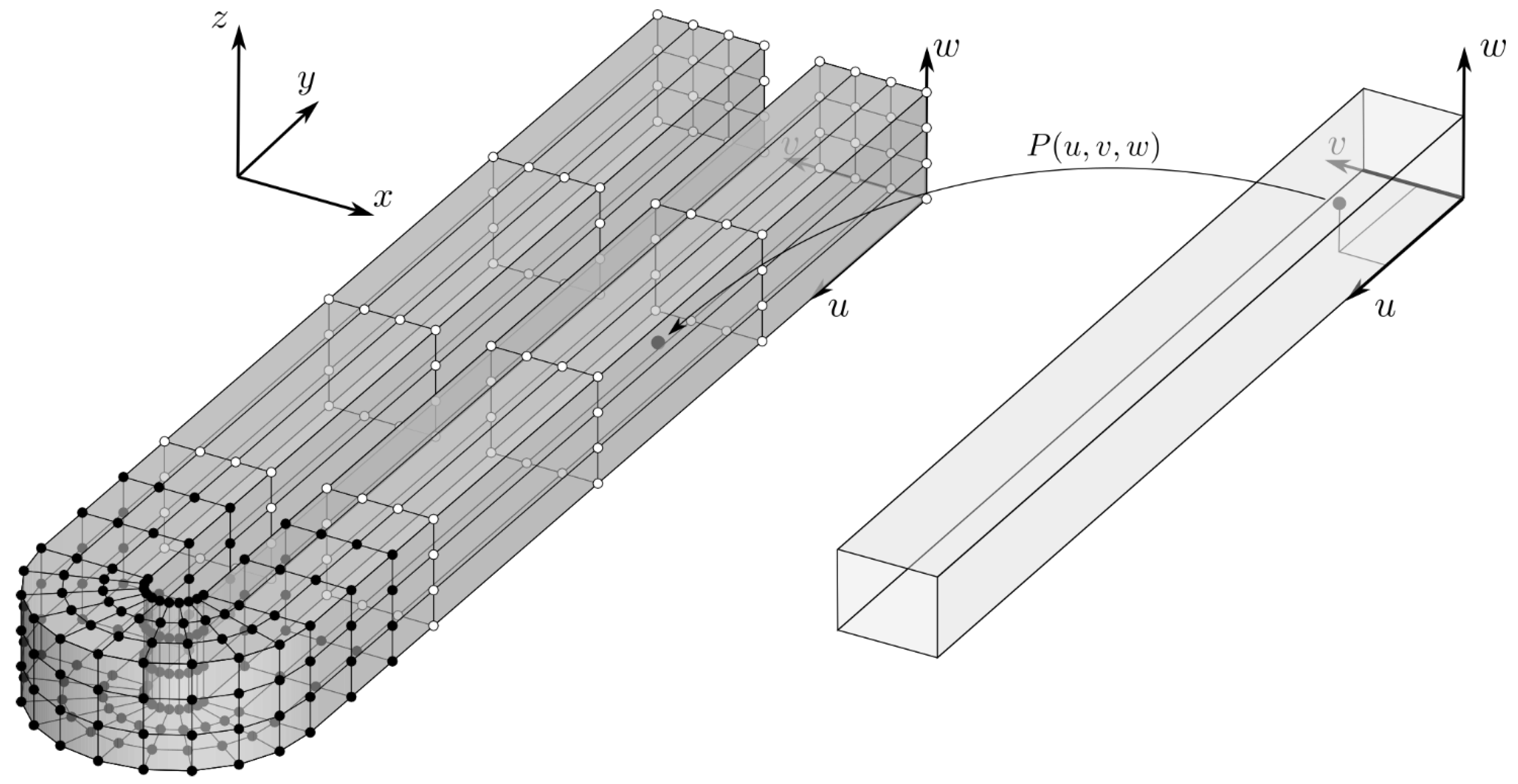
Figure 2 shows the mapping from the computational domain to the U-bend, as well as the external control points of the three dimensional array P_i,j,k. The skin of the volume is composed of six faces, which can be easily expressed as B-spline surfaces by setting u equal to either u₀ or u₁ in Equation (1), and likewise for v and w.

The parameters controlling the shape of the U-bend are the external control points of the tri-variate B-spline marked in black in Figure 2, totalling 180 free control points each with three degrees of freedom, resulting in a total of 540 degrees of freedom. The internal control points are repositioned based on a transfinite interpolation from the exterior control points, as follows:

$$\begin{array}{cc}{P}_{i,j,k}=& (1-i/m_u)·P_{0,j,k}+(i/m_u)·P_{m_u,j,k}+(1-j/m_v)·P_{i,0,k}+(j/m_v)·P_{i,m_v,k}\\ & -(1-i/m_u)·(1-j/m_v)·P_{0,0,k}-(1-i/m_u)·(j/m_v)·P_{0,m_v,k}\\ & -(i/m_u)·(1-j/m_v)·P_{m_u,0,k}-(i/m_u)·(j/m_v)·P_{m_u,m_v,k}\\ & for i=1\dots m_u-1,j=1\dots m_v-1,k=1\dots m_w-1.\end{array}$$

(5)

Transfinite interpolation is usually used to generate a grid based on points located at the external boundaries of the domain. In the present application, however, it is used to position internal control points based on the position of the external control points—this applies for every position of the k-index.

2.2. Grid Generation

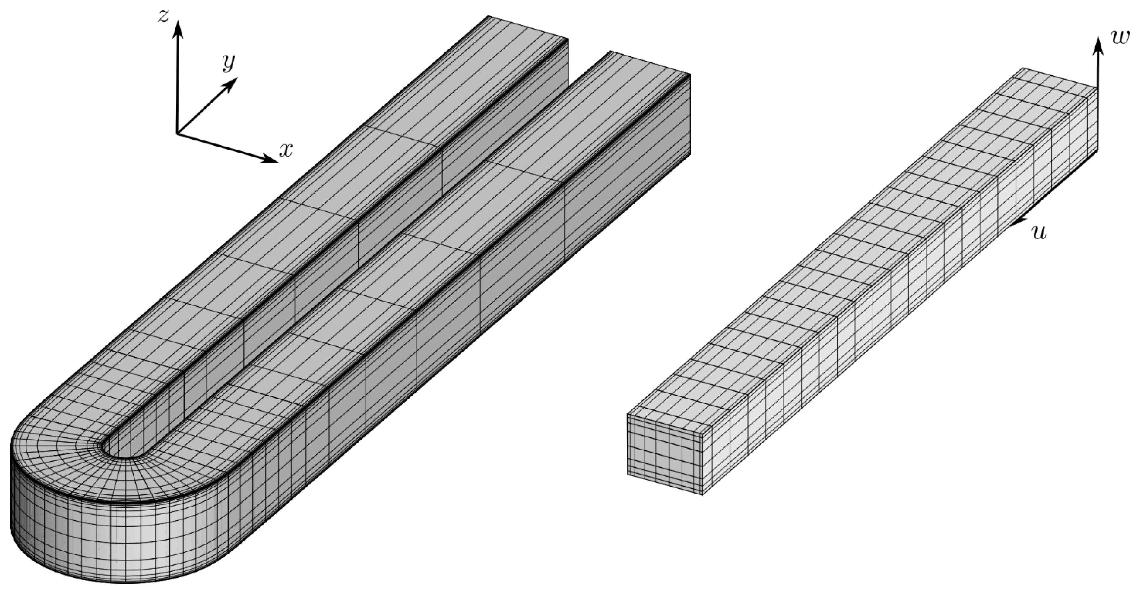
The use of tri-variate B-splines enables the establishment of a mapping between the computational domain and the U-bend shape. The generation of a structured mesh is, as a result, a straightforward task and requires the generation of a structured mesh in the computational domain only, as illustrated in Figure 3. A stretching is applied in the (v,w)-directions to allow for a boundary layer refinement suitable for a low Reynolds turbulence model, required to correctly predict the secondary flow structures. A grid with 200 × 64 × 64 cells is used in the u,v,w directions respectively, resulting in 819,200 cells.

2.3. CFD Solver

The Reynolds-Averaged Navier-Stokes equations are solved on multiblock structured grids with a cell-centered finite volume formulation, based on an adaptation of the JT-KIRK scheme of Xu et al. [22]. Convective fluxes are computed using Roe’s approximate Riemann solver [23] with a MUSCL-type reconstruction [24] of primitive variables for second-order accuracy. Oscillations are suppressed by a van-Albada type limiter [25], while the numerical dissipation of the scheme is controlled by the entropy correction of Harten and Hyman [26]. Viscous fluxes are computed with a central discretisation scheme. The turbulence closure problem is realised with the negative Spalart-Allmaras turbulence model [27], assuming fully turbulent flow from the inlet (Re = 40,000, based on the hydraulic diameter).

Geometric multigrid is used to damp low-frequency spatial modes, hence speeding up the convergence. Implicit time integration is applied on each multigrid level using a GMRES solver with ILU(0) preconditioning, while the system matrix is the first order Jacobian to reduce the stiffness of the solve. The GMRES solver is embedded in a Runge-Kutta multi-stage time integration method to damp high-frequency temporal modes, which a single stage GMRES solver would fail to do.

2.4. Adjoint Solver

After converging the CFD solver, the pressure loss induced by the U-bend can be readily computed at the domain outlet as:

$$J=\underset{S_{out}}{{\displaystyle \iint }}\frac{p}{{\rho }^{\gamma }} dS,$$

(6)

which is proportional to the entropy generation, and needs to be minimised. It is required to compute the derivative of this objective with respect to every design variable α. To compute the derivative with respect to an arbitrary design variable α, we make use of the chain rule:

$$\frac{dJ}{d\alpha }=\frac{\partial J}{\partial \alpha }+\frac{\partial J}{\partial u}·\frac{du}{d\alpha },$$

(7)

with u representing the flow variables $\left(\rho ,\rho ·\overline{V},\rho ·e\right)$. Quite often $\frac{\partial J}{\partial \alpha }=0$ because the objective function does not explicitly depend on the design variables. In the present case the outlet is located far away from the zone affected by the design variables, such that this term indeed vanishes. Note, as well, that Equation (7) has to be seen schematically, as the flow variables depend on the position in the domain. Hence, in a discretised form u is a large vector containing the flow variables of each grid cell, while for a continuous derivation Equation (7) needs to be replaced by considering the chain rule inside the integral of Equation (6). We therefore opt to consider the discrete problem from here on, which leads to the derivation of the discrete adjoint.

The two partial derivatives of J on the right hand side in Equation (7) can be directly computed, while the last total derivative of u can only be computed by looking at the Navier-Stokes equations. We assume that the steady-state governing equations are expressed in a residual form:

$$R\left(u,\alpha \right)=0.$$

(8)

This equation relates the flow solution to the design variables and describes how the flow variables change when a design variable is altered. The relation has to still hold for an infinitesimal change to a design variable:

$$\frac{\partial R}{\partial \alpha }+\frac{\partial R}{\partial u}·\frac{du}{d\alpha }=0.$$

(9)

Equation (9) is a linear system of the unknown $\frac{du}{d\alpha }$, which can be solved using classical linear system solvers. After inserting the result in Equation (7), the sensitivity of the design variable α is obtained. We need, however, to repeat the process for all other design variables, requiring an expensive linear system solve each time. The computational cost is, as a result, dependent on the number of design variables. By using the adjoint approach (Pironneau [28]), however, one can reduce the computational cost to only one linear system solve of the adjoint equation:

$${\left(\frac{\partial R}{\partial u}\right)}^T·v={\left(\frac{\partial J}{\partial u}\right)}^T.$$

(10)

Using the solution v^T to this linear system:

$$\frac{dJ}{d\alpha }=\frac{\partial J}{\partial \alpha }-v^T·\frac{\partial R}{\partial \alpha }$$

(11)

allows us to compute the gradient with respect to all design variables with only one linear system solve. The proof is fairly simple and relies on writing the solution of Equation (9) explicitly and putting it into Equation (7):

$$\begin{array}{ccc}\frac{dJ}{d\alpha }& =& \frac{\partial J}{\partial \alpha }+\frac{\partial J}{\partial u}·\frac{du}{d\alpha }\hfill \\ & =& \frac{\partial J}{\partial \alpha }-\frac{\partial J}{\partial u}·\left({\left(\frac{\partial R}{\partial u}\right)}^{-1}·\frac{\partial R}{\partial \alpha }\right)\hfill \\ & =& \frac{\partial J}{\partial \alpha }-\left(\frac{\partial J}{\partial u}·{\left(\frac{\partial R}{\partial u}\right)}^{-1}\right)·\frac{\partial R}{\partial \alpha }\hfill \\ & =& \frac{\partial J}{\partial \alpha }-v^T·\frac{\partial R}{\partial \alpha }\hfill \end{array}$$

(12)

Close examination of Equation (10) reveals that the system matrix on the left hand side is the Jacobian of the fluxes of the primal CFD solver. The fluxes are obtained using a second order Roe scheme and a central scheme for the viscous fluxes, such that the stencil spans over a large number of neighbouring cells. This leads to a sparse Jacobian, though, with entries that are far off-diagonal. The system is very stiff and difficult to solve with a direct solver and often prohibitive due to memory limitations. Therefore, the adjoint equations Equation (10) are solved with the same iterative time marching method as the primal CFD solver (Nielsen et al. [29]). A further simplification is introduced by a frozen turbulence approach, which assumes the turbulent viscosity to remain invariant to the changes in the geometry.

2.5. Computation of the Grid Sensitivities

The solution of Equation (10) provides the adjoint flow variables v, but the computation of $\frac{\partial R}{\partial \alpha }$ is still required in Equation (11) to obtain the sensitivities of $J$ with respect to the design variables. This term expresses how the residual changes under a perturbation of a design variable, through the mechanism of changing each node’s coordinates which changes each face normal and area, and each cell volume. It can be computed by a forward approach, i.e., by changing each design variable individually and multiplying the computed term with the adjoint variables v as in Equation (11) to obtain the sensitivities for each design variable. Although in general such a procedure is relatively fast, it needs to be repeated for each design variable and hence becomes less attractive for a large number of design variables. As an alternative, a reverse or adjoint procedure can be used here as well, similar to what has been applied to the CFD solver. A first step is to introduce the grid coordinates P of the mesh in the process (P here refers symbolically to the (x,y,z) coordinates of all grid nodes). The term can thus be written as:

$$\frac{\partial R}{\partial \alpha }={{\displaystyle \sum }}^{\text{}}\frac{\partial R}{\partial P}·\frac{dP}{d\alpha },$$

(13)

where the summation spans over all grid coordinates. Because a change in one grid coordinate has only a local effect to its neighboring cells, the term $\frac{\partial R}{\partial P}$ can be obtained both in forward or reverse mode. This is typically done as a post-processing step in the adjoint CFD run. The result is the sensitivity of the objective function with respect to each grid coordinate:

$$\frac{dJ}{dP}=-v^T·\frac{\partial R}{\partial P}.$$

(14)

This value is referred to as the adjoint grid coordinate value and is available in each grid point P after computing Equation (14).

In the next step, the term $\frac{dP}{d\alpha }$ is considered by including the tri-variate B-spline control points in the process:

$$\frac{dP}{d\alpha }={\displaystyle \sum }_{i,j,k}\frac{dP}{d{P}_{i,j,k}}·\frac{d{P}_{i,j,k}}{d\alpha }.$$

(15)

By using Equation (1) we can compute $\frac{dP}{d{P}_{i,j,k}}$, which in turn allows to compute the adjoint to the control points starting from the adjoint grid coordinates:

$$\frac{dJ}{d{P}_{i,j,k}}=\frac{dJ}{dP}·\frac{dP}{d{P}_{i,j,k}}.$$

(16)

This requires only the evaluation of the basis functions as expressed by Equations (2) and (3) for each grid point, which can be computed in a considerably shorter time compared to one CFD iteration. Alternatively, these sensitivities could be stored in memory, which has not been applied in the present work.

2.6. Computation of the Design Variable Sensitivities

The sensitivities of the objective function with respect to all control points of the tri-variate B-spline are given by Equation (16). The design variables in this test case are limited to the control points on the skin of the U-bend, i.e., the surface that is allowed to change, thus excluding the long inlet and outlet legs (see Figure 2). The design variables are thus the control points P_i,j,k, with restrictions to certain indices:

$$\alpha =P_{i,j,k} with \{\begin{array}{c}i=i_{min}\cdots i_{max}\\ j=0\cdots n_v for k=0 or k=n_w\\ k=0\cdots n_w for j=0 or j=n_v\end{array}.$$

(17)

To compute the sensitivities w.r.t. (the moveable control points), we make use of Equation (5) to obtain:

$$\frac{dJ}{d\alpha }=\frac{dJ}{d{P}_{i,j,k}}·\frac{d{P}_{i,j,k}}{d\alpha }.$$

(18)

2.7. Steepest Descent

Through the gradient computation described above the linearized behaviour of the objective function in the vicinity of the current design is known. It allows modification of the design in the direction of steepest improvement:

$${\alpha }_{i+1}={\alpha }_i-\lambda ·\frac{dJ}{d\alpha },$$

(19)

where a step size λ is taken small enough to ensure reduction of the objective. This method, known as the steepest descent method, is recognised to converge slowly to the optimum. We include here, however, the process of geometry modification by the steepest descent into the cycle of converging the CFD and adjoint solvers, resulting in what is called a one-shot method (Hazra, [30]). Ten iterations of the CFD and adjoint solvers are performed before an update to the geometry is made. The update is bound to be rather small to be able to reuse the last CFD and adjoint result as a restart for the next iteration. This is only effective in the present case due to the very fast grid generation process and computation of grid sensitivities.

3. Results

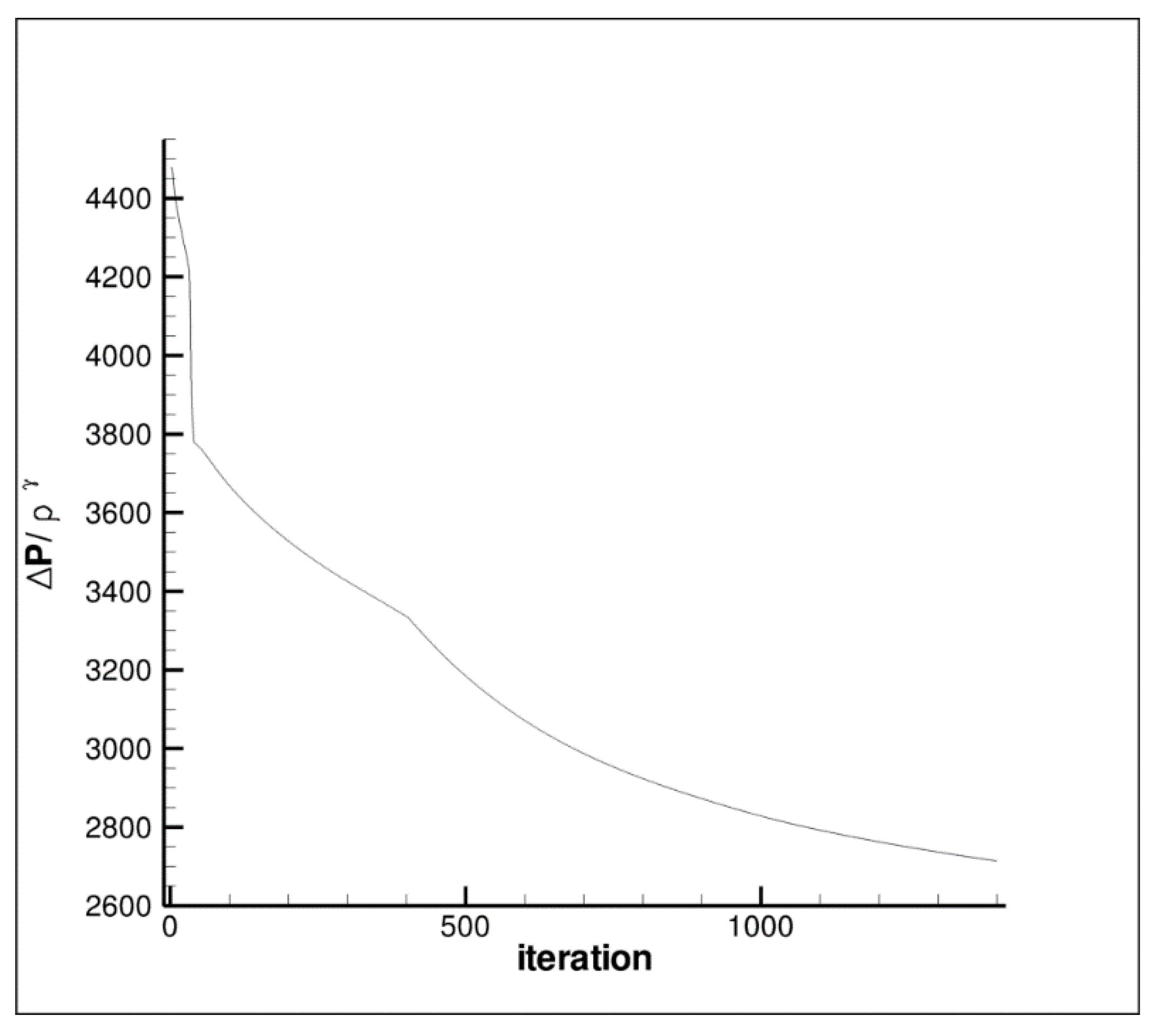
Figure 4 shows the convergence history of the objective function (Equation (6)) for each cycle of the optimisation as depicted in Figure 1 (after 400 iterations the step size has been increased, hence the kink). After 1400 cycles, or 14000 CFD and adjoint iterations, the process is stopped. The baseline and final configuration are compared in

Table 1. Comparison of baseline and optimal geometry.

	Baseline	Iteration 1400	Relative Improvement
$\mathrm{\Delta }\frac{p}{{\rho }^{\gamma }}$ (-)	4478	2714	39.0%
$\mathrm{\Delta }p$ (Pa)	1258	772	38.6%
$\dot{m}$ (Kg/s)	0.1078	0.1303	20.9%
$\frac{1}{2}\rho v^2$ (Pa)	885	1318	48.7%
$\frac{\mathrm{\Delta }\mathrm{p}}{\frac{1}{2}\rho v^2}$ (-)	1.421	0.586	58.7%

. A total reduction of 39% in entropy generation is achieved, while at the same time (since a static pressure boundary condition is imposed at the exit), the mass flow increases by 20.9%. The combined effect of pressure loss decrease and mass flow increase can be considered by looking at the non-dimensional pressure loss coefficient $\frac{\mathrm{\Delta }\mathrm{p}}{\frac{1}{2}\rho v^2}$, which decreases by nearly 60%. It needs to be noted that the Reynolds number also increases by 10%, which needs to be assessed for a direct comparison.

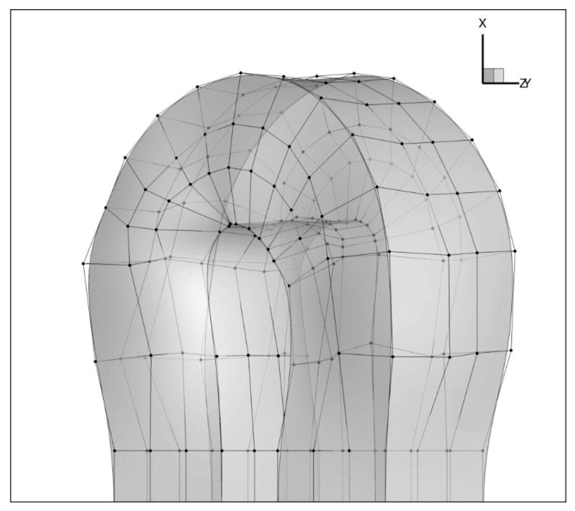
Figure 5 shows the deformed geometry together with the control points. A clear feature is the increased width of the space in between the forward and return channel, as well as the curved shape of the end wall near the 90 degree position of the bend.

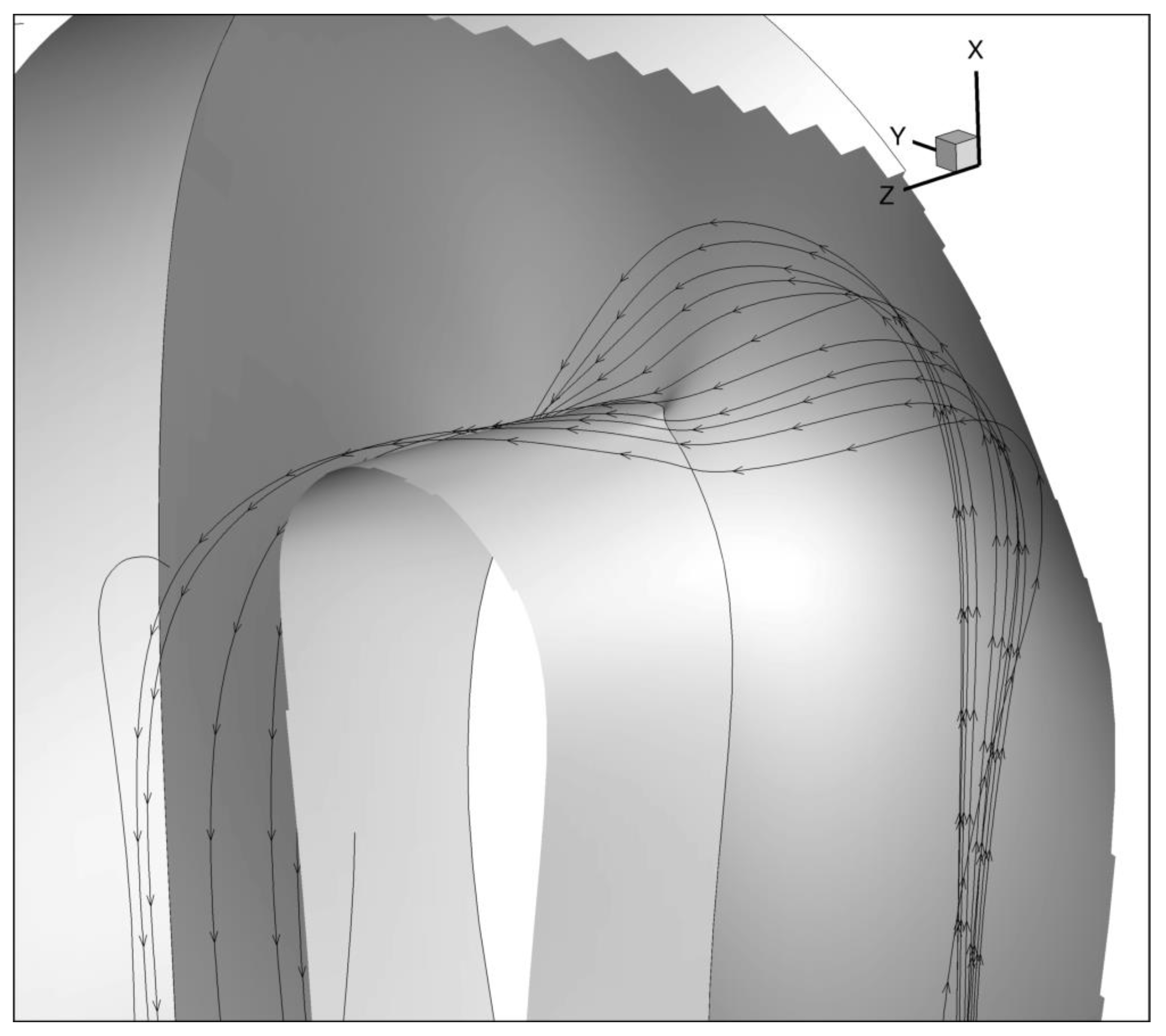
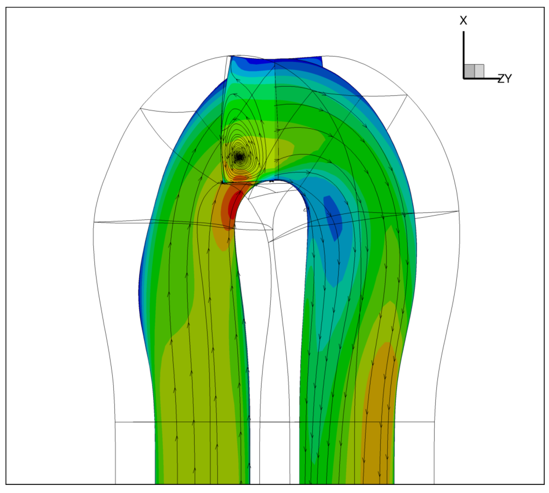
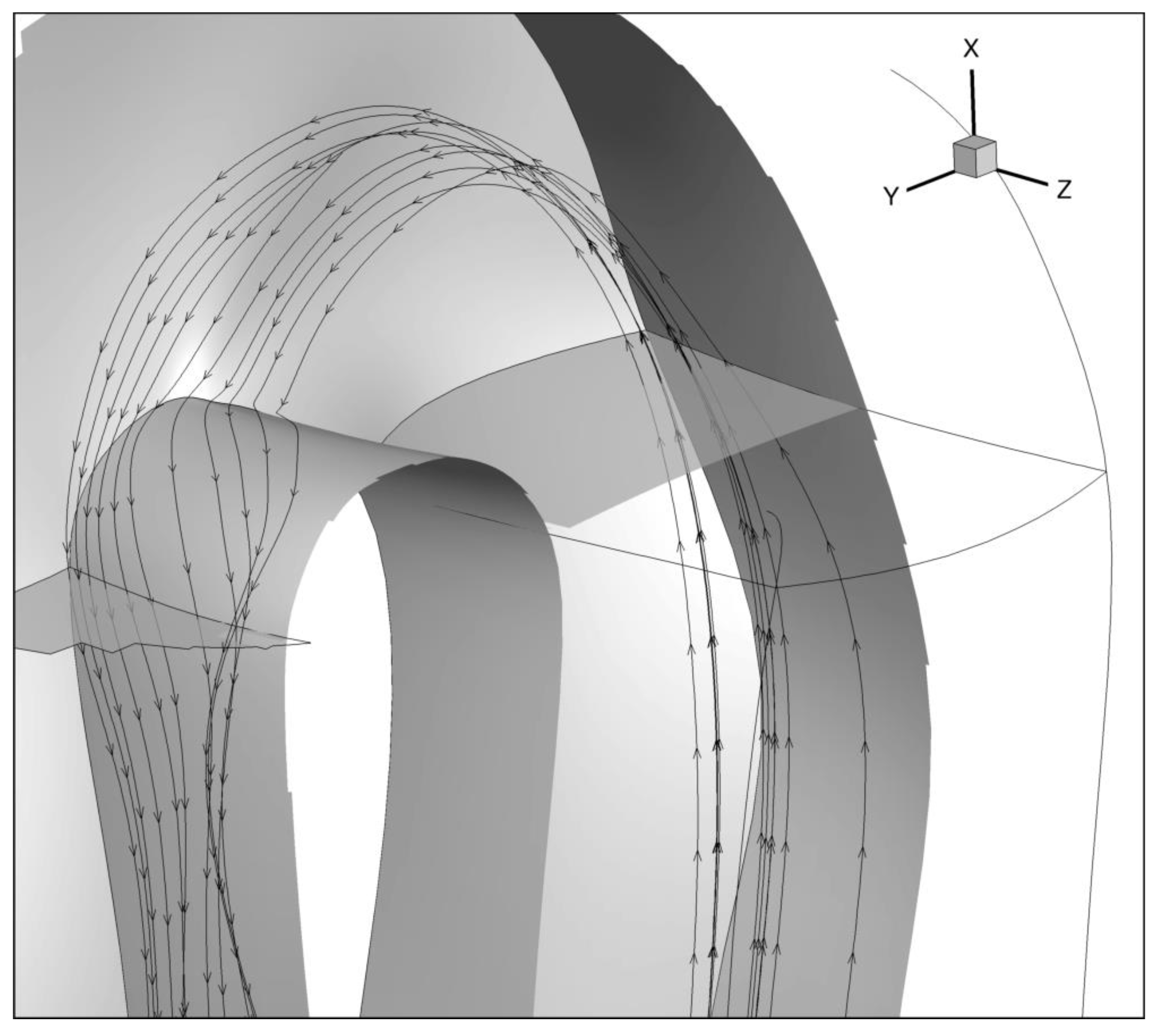
Figure 6 shows the velocity magnitude in the mid plane of the channel, as well as the secondary flow structure in the 90 degree position of the U-bend. It can be seen that the separation in the second part of the bend, present in the baseline shape, has been successfully reduced. We attribute this reduction to mainly three effects. First, due to the increased space in between the forward and return channel, a bend results for which the curvature in the lower part of the bend is strongly reduced. Because for incompressible, irrotational flow, the velocity gradient normal to the streamline is proportional to the curvature of the streamline, the enhanced radius of curvature results in a more gradual velocity increase from inner wall to exterior wall. This results in a lower acceleration of the flow along the first part of the inner wall, and hence a less aggressive adverse pressure gradient along the second half of the turn. Secondly, the cross-sectional area decreases in the streamwise direction in the first 90 degrees of the bend, defusing the flow and additionally reducing the acceleration on the inner part of the U-bend. In the second half of the bend a contraction of the channel follows, reducing additionally the above mentioned deceleration in an adverse pressure gradient. Finally, a third contribution is obtained by shaping the four endwalls more smoothly by removing the sharp 90 degree corners to help the secondary flows re-energise the low momentum flow in the second half of the bend. In Figure 7 and Figure 8 the streamlines of such secondary flow are illustrated, and (as can be seen) the flow entering the low momentum region originates from a part far away from the wall in the inlet part of the bend. Hence, this flow consists of high momentum and will re-energise the low momentum flow present at 90 degrees. The shape at the endwall helps this flow to turn sharply from the endwall into the low momentum region.

4. Conclusions

A novel parametrisation method has been introduced which uses tri-variate B-spline volumes to deform shape and volume mesh. This parametrisation ensures a rich design space while maintaining the geometry description in CAD format. Due to its cheap and robust grid generation process, the method can be incorporated efficiently in a one-shot method which simultaneously converges flow, adjoint and design. The computational cost of obtaining the flow in the optimised shape is 10 times the cost of computing flow and surface sensitivities (adjoint) of the baseline configuration.

The method has been applied to minimise pressure losses of an internal cooling channel U-bend with 540 degrees of freedom. Sensitivities of the objection function with respect to the CAD parameters are evaluated using the adjoint approach for flow solver, mesh generation and shape parametrisation. A reduction of 39% in pressure loss was achieved while, at the same time, the mass flow increased by 21%, leading to a non-dimensional reduction in losses of 59%. Finally, the optimised bend shape remains available in CAD format, allowing a straight forward process to manufacture the optimal shape.

The method is a significant step forward in building high-fidelity shape optimisation workflows as it removes two major bottlenecks. Firstly, the use of tri-variate B-Splines to deform shape and volume consistently provides a robust method of mesh deformation at very low computational cost. Secondly, both the initial and final shapes are defined in a CAD representation which avoids any manual shape approximations in CAD that may lose optimality and are labour-intensive. Instead, the optimal shape can be used directly for further analysis or manufacturing.