Beyond Housing Preferences: Urban Structure and Actualisation of Residential Area Preferences

Abstract

The concept of residential housing preferences has been studied across multiple disciplines, with extensive literature supporting both stated and revealed preference methods. This study argues that both preference types, stated and revealed, should be assessed concurrently to achieve a more comprehensive understanding of residential housing choices. To provide evidence, this research used findings from a public participation GIS survey that identified the stated housing preferences associated with three categories of urban residents, which were called urban “tribes”. We implemented an analytical framework using fuzzy modelling to relate stated preferences with revealed preferences for the same individuals using empirical data describing the urban structure in Tampere, Finland. Following an analysis of the relationships between residents’ revealed preferences and urban structural variables, we examined the consistency of stated housing preferences with revealed preferences. The results show considerable mismatch between the stated and revealed preferences for the urban tribes that were examined i.e., the preferred housing environment was significantly different from the actual living environment. Further, the stated preferences showed disequilibrium within the current structure of the housing supply in Tampere. The findings can have important implications for housing policy making in Tampere. Further, the use of a novel fuzzy model approach demonstrated a flexible and tolerant method for working with imprecise and variable social data to capture subtle differences. Finally, this study elaborately discusses the remaining limitations and suggests how they should be addressed in future research.

1. Introduction

With increasing global urbanisation, the quality of life in urban environments has emerged as one of the main concerns of urban planners. The crucial influence of urban structure on the perceived quality of urban settings has been identified by some researchers [1,2,3] such that when the characteristics of the living environment meet expectations and preferences, the good fit leads to greater satisfaction and higher quality of life [4]. However, studying whether living environments fit public preferences is challenging. With considerable diversity in individual perceptions of place and the potential to pursue multiple social lifestyles, people’s preferences and evaluations of their living environment are also becoming increasingly diversified [4]. This heterogeneity of perceptions and preferences has influenced the demand for variegated housing environments that can challenge the existing structure of urban areas. To provide insight into how people choose their housing location, residential environmental choice has been a focus of scholarly research.

Residential preferences have been extensively studied from various perspectives by researchers from different disciplines [5]. In many studies, demographic and socioeconomic variables have been identified as primary determinants of preferences [6]. Demographic variables have an obvious influence on residential preferences, because household composition is related to housing needs [7]. As the size and composition of a household change, residential preferences may change as well [6]. Socioeconomic variables have been examined using residential segregation research with variables such as income, education, and race/ethnicity [6,7,8,9]. According to these studies carried out in Los Angeles (United States), a strong desire for own-race neighborhoods was evident among different ethnic groups. However, these studies also identified that as the level of income and education increase, the probability of choosing a more integrated residential setting (race/ethnicity) also increases [8].

However, sociodemographic variables cannot fully explain housing preferences. Some studies have found that people with similar sociodemographic profiles have different residential preferences [10,11]. Furthermore, as Jansen and Heijs et al. argue [12,13], given the considerable cultural and economic changes that have taken place in western countries in recent decades, the variety in housing choices has significantly broadened. Consequently, traditional sociodemographic characteristics may no longer suffice for explaining and predicting residential preferences [12]. In response, a number of studies have analysed preferences using lifestyle variables. In these studies, lifestyle variables are proposed as an intermediary in the translation of sociodemographic characteristics into consumer preferences that fill the gap between traditional variables and the cultural aspects of life [4,13,14,15,16]. Lifestyle variables make it possible for urban planners to better identify the relationship between the characteristics of urban settings and the residential choices of inhabitants.

In addition to sociodemographic and lifestyle variables, geographical variables may also influence residential preferences. When selecting a place to live, people choose a certain type of residential area. Accordingly, housing choice has a significant geographical aspect. Therefore, cities may be defined as physical structures whose spatial changes are both the cause and the result of residential mobility [6,17,18]. Dieleman [19] highlighted the importance of geography in how people make residential choices. The author argued that the relationship between geography and residential choice is recursive [19]. That is, circumstances over space and time influence the housing choice patterns of individuals and households, and vice versa. Later, Dieleman and Mulder [20] presented a qualitative approach for studying the geographical aspect of residential choices. They argued that it is possible to estimate residential mobility based on the geography of residential environments [20]. Clark et al. [21] expanded on this idea by examining the relative role of the physical environment in residential choice, and used a quantitative approach to model this relationship. They found that in residential mobility, not only do people look for better socioeconomic status, they also tend to move towards an enhanced environmental quality of the neighbourhood (less density, more greenspace). Nevertheless, the body of housing research focussing on geographical aspects is considerably smaller than the research that focussed on its economic aspects [18,22,23].

In residential choice research, there is an obvious distinction between revealed and stated residential preferences [24]. The outcome of a housing decision is often referred to as a revealed preference [6,24,25]. This contrasts with the stated preference that is determined by asking people directly their preferences for housing [6,24], e.g., through a survey. Measuring revealed preferences is rather straightforward, and is achieved by modelling the observational data of households’ actual housing choices [25]. Studies adopting revealed preferences are based on the assumption that people can best express their housing preferences through the places they choose to live [26]. However, some researchers believe that this approach does not adequately explain what people truly prefer [27]. For this reason, stated preferences are important to study as well.

However, despite the arguments on the advantages of studying stated preferences to identify implicit residential preferences, revealed preferences remain the dominant approach in housing mobility research. This could be partly due to the difficulty of identifying relationships between stated preferences and the physical environment [6]. In addition, some studies argue that stated preferences are typically biased towards revealed preferences [28]. In other words, the longer people reside in a certain type of housing, the more likely it is that their stated preferences match the revealed ones. This might suggest that studying stated preferences may not render new understanding. However, these arguments have remained inconclusive to this point, as both stated and revealed preferences are widely used in the literature. This may indicate a need for moving towards more integrative approaches [29], replacing the current attempts on dismissing one approach or the other.

Aim of the Study

The aim of this study is to present a novel method for integrating stated and revealed preference data to provide a better understanding of residential area preferences. The need for the integration of these two preference types for housing studies was formerly identified in some earlier studies [29]. Stated and revealed preference methods are common in housing choice research, but arguably, neither approach is sufficiently comprehensive to fully explain housing decisions. Stated preference studies often include sociodemographic and lifestyle variables, but do not typically focus on physical environmental variables. In contrast, revealed preferences are directly linked to the physical environment, but often do not fully incorporate participant variables. For a better understanding of the contribution of both participant and environmental variables in residential preferences, we present a new analytical framework. This framework is based on the assumption that both stated and revealed residential preferences should be measured and included in the analysis.

The stated preferences in this study were identified using a clusterisation of individuals into three “urban tribes”, as previously published by Haybatollahi et al. [30]. An online map-based survey was used to identify these tribes as well as measure the revealed preferences based on the actual living locations. Consequently, we chose to implement a fuzzy logic model wherein the physical environment serves as a connecting layer between stated and revealed preference methods. The supporting rationale is that a fuzzy logic approach accounts for uncertainty in preference analysis while accommodating the complex, nonlinear functions that are present in this study, and can extract useful information from a dataset that is not of highest statistical reliability. However, a limitation of fuzzy logic modelling is that similar to its name, the results may also be “fuzzy” and require subjective interpretation and inference.

The empirical analysis of this study is based on data collected in the city of Tampere, which is the second largest city in Finland. The objectives of this study are fivefold:

(1)

Present an analytical framework that accommodates the concurrent investigation of stated and revealed preferences for housing areas.

(2)

Develop a quantitative modelling method that can analyse imprecise and variable social data while still revealing primary information.

(3)

Estimate the overall extent of (dis)equilibrium between revealed residential preferences and residential opportunities offered by the current urban structure in Tampere.

(4)

Examine the overall congruence between stated preferences (from survey data) and revealed preferences and assess the extent to which the current urban structure matches the two preference types.

(5)

Describe the strengths and limitations of the analytical approach for integrating stated and revealed preference data.

Answering these questions will help researchers investigate the equilibrium between the stated and revealed preferences and demonstrate the relevance of an integrative approach. Further, within this scope, this study will demonstrate how such an integrative approach can be realised through novel methods. In addition to these more general research contributions, this study will also empirically examine the residential opportunities offered by the current urban structure in Tampere and evaluate its (dis)equilibrium with the residential preferences of the residents.

2. Materials and Methods

A conceptual overview of the study design is presented in Figure 1, which aims to link stated and revealed preference data to determine the degree of congruency in the two methods. The relationship between urban structure and revealed preferences was analysed through statistical observations and the development of a fuzzy logic model. Stated and revealed preferences were compared to assess the degree of their congruency in predicting housing preferences.

The relationship between urban structure and revealed preferences was examined for four urban structural variables: population density, green area percentage, non-motor routes density, and service point density. Following visual mapping, statistical measurements and observations were used as inputs to construct a fuzzy model to estimate how revealed preferences and urban structure match.

The stated preference data used a typology developed by Haybatollahi et al. that has been derived from survey data where study participants were asked about their residential preferences [30]. Stated neighborhood preferences were measured using 10 attitudinal statements (see Figure 2) formulated based on living the environment preference scale that was developed in a qualitative study on two Finnish neighborhoods [31]. Subsequently, participants were classified into three clusters: so-called “urban tribes” representing different residential and neighbourhood preferences [30]. Using this typology of stated preferences, this study determined the congruence between stated and revealed preferences. This was done by identifying the number of individuals who live in locations where the presence of the different urban structural variables matched their stated preferences.

2.1. Study Area and Datasets

The empirical study was conducted in Tampere, the second largest city in Finland with a metropolitan population of 313,058 (Statistics Finland, 2011). Spatial data was collected and prepared for analysis from a number of different sources. Population data from the census was disaggregated and analysed as the number of people living in 1 × 1 km grids within the study area. Data on green areas was extracted from the SLICES dataset obtained from the National Land Survey of Finland (2010). Parks, forests, and agricultural fields were considered as green areas, and the percentage of green area was calculated for each grid cell. Walking and cycling route data were collected from Open Street Map with the density of routes calculated as km per 1 km². All of the values were scaled using a multiplication by 10³ to facilitate calculation with larger values.

Service data, which was represented as points, was collected from the City of Tampere. The data included all classes of public and private services (e.g., public transportation, shops, schools, and day care centers). Service density was calculated as the number of service points located within each grid cell. The values were scaled by 10⁵ to facilitate calculation. Data for buildings was obtained from the Tampere municipality and contained comprehensive information including building type, floor area, and year of construction. This information was used to normalise the model results so that the definition of the area also included the built environment.

2.2. Public Participation Data and Cluster Analysis

The survey data was collected in summer 2012 as part of a larger study to investigate the relationships between residential preferences and travel behaviours [30]. A random sample of 20,235 inhabitants living in Tampere metropolitan area with an age range between 15–74 years was obtained from the Finnish Population Register Centre. All of the sample members received a postcard via mail to their home address inviting them to participate in the survey. The SoftGIS method was employed in the survey, which incorporated a customised questionnaire with the map. SoftGIS is an example of public participation GIS (PPGIS) method that enabled the combination of ‘soft’ subjective data with ‘hard’ objective GIS data [32]. This facilitates the collection of large datasets for use by urban planners and other professionals who are interested in the development of more user-friendly physical settings [32]. This method has been used in several Finnish cities as well as in Japan, the United States (USA), and Australia [33,34,35,36]. In this specific study, participants were requested to identify and map their current home locations as well as places they visit on a regular basis (e.g., service points, work, etc.). The survey consisted of four sections that were designed to gather information concerning the residential and mobility prospects, as well as basic background and demographic information. For more details about the data acquisition process, the readers are referred to [30].

A total of 3403 inhabitants of Tampere (17% response rate) participated in the survey. Participants were mostly homeowners (64.2%) rather than tenants (32.2%), with about half of participants living in single occupant households. About 53.2% of participants were employed, 19.6% were retired, 15.6% were students, 5.6% were unemployed, and 2.8% were stay-at-home parents. Participants had some bias compared to the population structure of the city where male respondents (44%) and the youngest age group (15 to 24) were slightly under-represented.

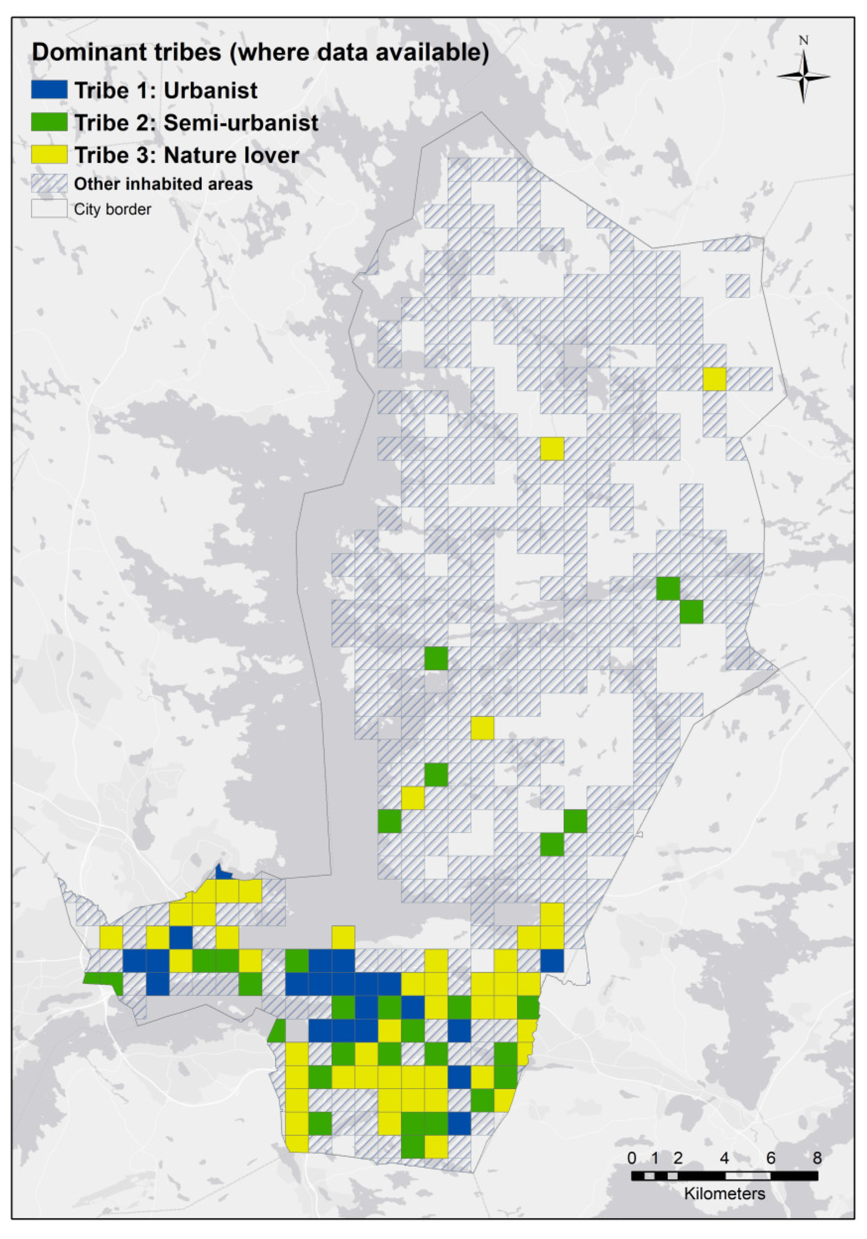
In the survey, the respondents were asked to scale their level of agreement with each attitudinal statement using a slider ranking from 0 to 100. Using responses to these 10 survey questions, Haybatollahi et al. identified three clusters of Tampere residents based on individuals’ neighbourhood and residential preferences [30]. In this paper, we refer to these clusters as urban tribes with the labels of urbanist, semi-urbanist, and nature-lover (Figure 2). The three urban groups consist of 36%, 29%, and 35% of total survey participants, respectively.

As illustrated in (Figure 2), Tribe 1 (urbanists) are people with stronger preferences for public transport who value the liveliness of the urban environment and are more open to changing living locations. In contrast, Tribe 2 (semi-urbanists) and Tribe 3 (nature lovers) have stronger preferences for private transport, greater appreciation for a calm and tranquil living environment, and seek permanent settlement in an area. Tribes 2 and 3 are differentiated on their relative preferences for nature and the amount of socialisation with their neighbors.

2.3. Data Analysis and Modelling

To examine the relationship between the places where the urban tribes live in Tampere and the urban structural variables, statistical measurements were performed on the data. The tribes’ statistical standing for different urban structural variables helps us identify their overall revealed preferences for residential settings. All of the study participants allocated to the three urban tribes were included in the analysis. For each individual, the four urban structural variables were assessed using a 500-m radius from their domicile.

To describe revealed preferences using urban structure variables, a fuzzy modelling method was used. Fuzzy inference systems (FIS) are popular computing frameworks based on fuzzy logic [37], which have been applied in many decision support systems [38]. The popularity of FISs is mainly because of their closeness to human perception and reasoning, as well as their simplicity and intuitive handling [39]. This study uses the Mamdani fuzzy inference system, which is an example of intuitive knowledge-based FIS based on a set of linguistic IF_THEN rules obtained from an experienced human operator [40].

The uncertainties in the data and similarities between tribes, together with the complexity of functions used in this study, motivated the use of fuzzy logic. Fuzzy logic can model nonlinear functions of variable complexity, and is popular because of its tolerance for imprecise data [41]. This tolerance can be a significant asset in working with subjective social datasets representing individual perceptions of different geo-coded phenomena [42].

In fuzzy theory, membership functions (MF) serve as the building blocks of the model. MFs are responsible for the fuzzification process; hence, their definition is regarded as one of the most important steps in fuzzy modelling. In this study, we used both visual and spatial analytical methods to create the building blocks of the model [43]. For each urban structural variable, we examined the tribe’s statistics to assign a combination of multi-section linear and nonlinear functions that best represent tribe frequency histograms for each variable (Appendix A: Model’s membership functions).

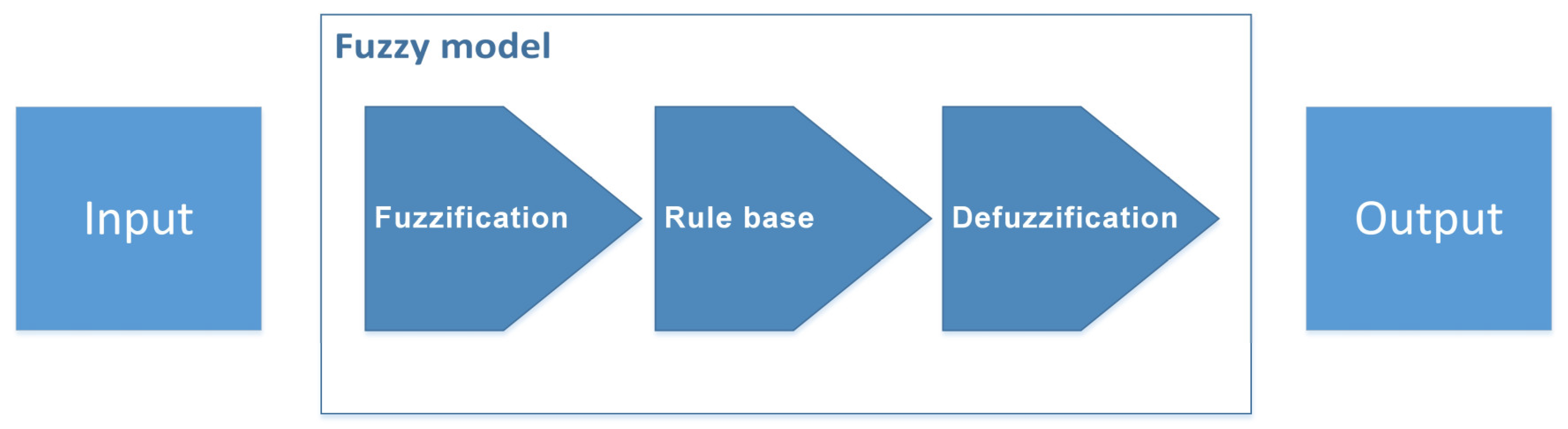
There are two general approaches for determining fuzzy rules: inductive and deductive [44]. In this study, we used a deductive approach, starting with general observations from data (rules), then progressing towards more specific hypotheses (weights) that were later confirmed by the model [45]. Accordingly, four IF-THEN rules were derived from the dataset to describe the connection between MFs and tribes. As illustrated in Figure 3, a fuzzy model was created using a “mean value of maximum” (MOM) defuzzification method and other model specifications (Appendix B: Model specifications). The MOM defuzzification method was customised to produce a single integer of one, two, or three, representing the assigned tribe number as the model’s output.

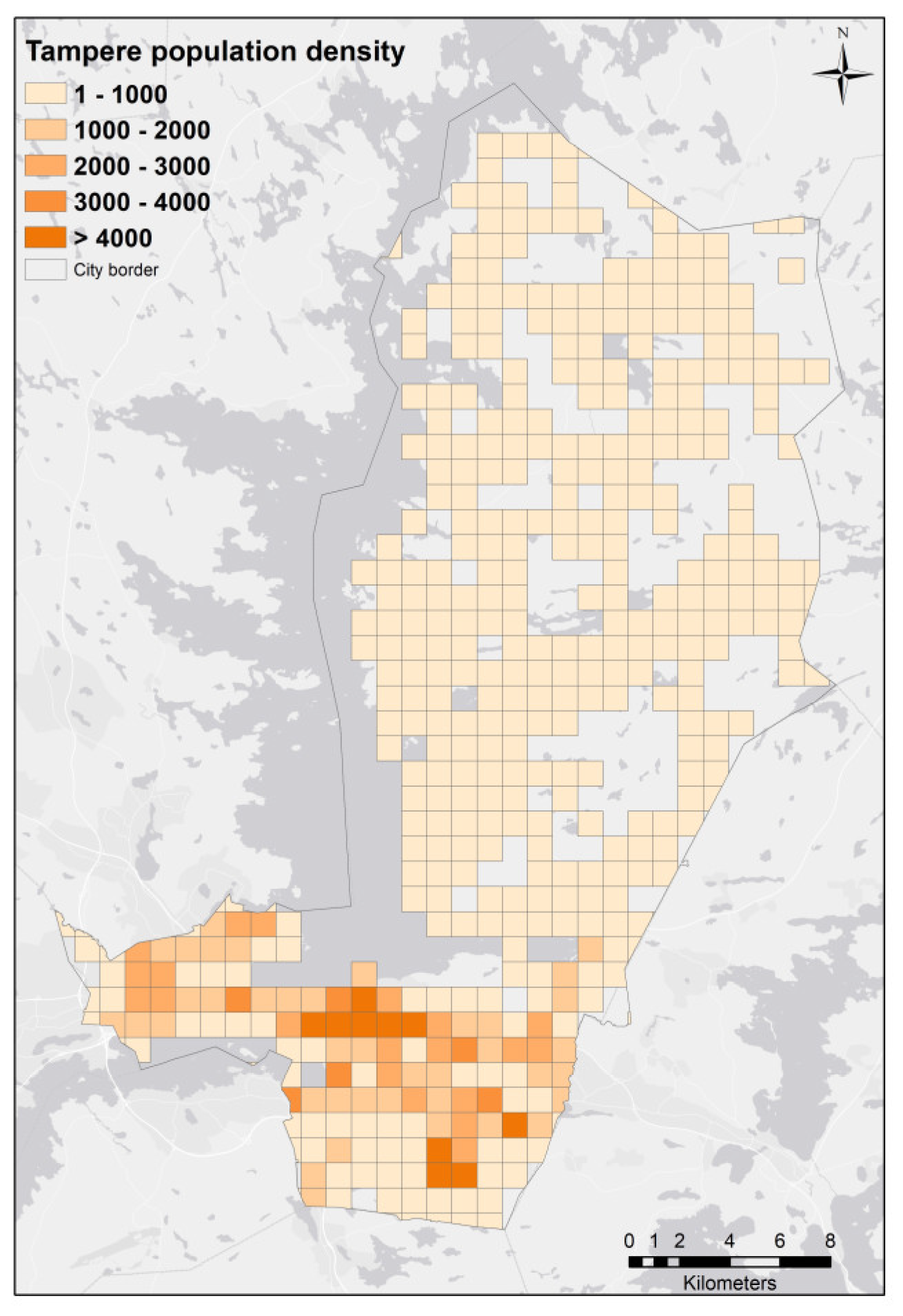
Subsequently, the developed fuzzy model was used to predict and estimate the compatibility of the urban structure in each population grid cell (Figure 4) to the tribes’ revealed preferences. For each cell, the four urban structural variables were used as inputs of the model to produce the most compatible tribe number as output. The input variables were normalised so that they would be independent from the cell areas. For this implementation, we used ‘adaptive neuro-fuzzy inference system’ (ANFIS) toolbox of Matlab R2015a software.

3. Results

3.1. Revealed Housing Location Preferences and Urban Structure

A visualisation of home location by tribe membership indicates that people belonging to Tribe 1 (urbanists) dominate the city center (Figure 5). To further examine the tribes’ geographical distribution, we created a dominance map (Figure 6) using 1 × 1 km grid cells. In this map, the dominance of tribes within each cell was determined by identifying the tribe possessing the largest number of home locations within the cell. In cases where a given cell contained an equal number of domicile points belonging to different tribes, a kernel density function was used as an alternative. As illustrated in these maps, the tribes’ geographical distribution has a generally radial pattern where urbanists dominate the city center, semi-urbanists predominantly live in suburban areas, and nature lovers dominate the periphery of the metropolitan area.

To quantitatively evaluate these observations and examine the potential relationship between the tribes’ housing location and urban structural variables, tribe-wise descriptive statistics were extracted from the data (

Table 1. Structural variables statistics for the three urban tribes.

	Urban Tribes (Count)
Urban Structural Variables	Measures	Tribe 1 Urbanist (359)	Tribe 2 Semi-urbanist (291)	Tribe 3 Nature lover (353)
Population density (Pop. Per km2)	Min	75	6	5
	Max	14,748	9125	9152
	Mean	4773	3494	2956
	Median	3886	2497	2021
	SD	2989	2630	2520
	Skewness	0.05	0.73	1.05
Green area coverage (%)	Min	0	2.5	0
	Max	76.5	79.2	88.8
	Mean	19.3	24.6	26.9
	Median	17.3	22.1	22.7
	SD	11.8	12.8	16.9
	Skewness	1.34	0.88	1.34
Service density (service points per km2) × 105	Min	0	0	0
	Max	184	190	214
	Mean	35.2	19.3	14.1
	Median	18	7	5
	SD	43.4	31.6	27.6
	Skewness	1.67	2.9	3.84
Non-motor route density (km of road per km2) × 103	Min	1784	389	489
	Max	34,888	34,475	33,589
	Mean	19,204	15,558	13,329
	Median	19,749	14,535	11,794
	SD	8078	7624	7265
	Skewness	−0.21	0.15	0.33

). To investigate the observations further, a multinomial logistic regression was also performed. Due to a high degree of variability in the urban structural variables that were used to predict group membership, the generated model rendered low statistical significance in most predictor variables. Therefore, it was left out of the study.

In line with Figure 5 and Figure 6, the housing choices of Tribe 1 members reveal their overall preference for living near the city center where the population density is higher, the green area coverage is lower, services are easily accessible, and where there is a higher density of non-motored routes. Tribe 3 members mostly inhabit peripheral areas where the population density is lower with a higher percentage of land covered by green areas. The revealed preferences of Tribe 2 fall in between the other two groups. This pattern can particularly be seen in the values for average and median (Table 1), on the urban structural variables. These indicate that the members of this urban tribe inhabit the transitional suburbs located between the city center and peripheral areas. These areas are not located in the city center, but have reasonable accessibility to the downtown area.

The largest distinction between the tribes’ revealed preferences was observed in their frequency histograms for each structural variables: these were used to render MFs (Appendix B). Although groups overlap in certain ranges, their overall urban structural profiles considerably differ from each other. This can also be seen in the calculated skewness values presented in Table 1, which shows the tribes’ overall distribution of urban structural variables.

3.2. (Dis)Equilibrium between Revealed Preferences and Tampere’s Existing Urban Structure

Using the fuzzy model developed in this study, we projected people’s revealed preferences to the whole city region (Figure 7). This was done by feeding the urban structural values into the model, which were calculated for each grid cell throughout the region. Based on the output of the fuzzy logic model, we identified the tribe that had the highest level of preference match with its urban structure for each grid cell.

Figure 7 shows how the urban areas matching each tribe’s revealed preferences are geographically distributed. More than 77% of the city’s inhabited areas match Tribe 3’s (nature lovers) revealed preferences, with significantly smaller areas matching Tribe 1 (urbanists) and Tribe 2 (semi-urbanists), with 14% and 9%, respectively.

A comparison of the land areas matching the revealed preferences of the three tribes and their respective sizes in the dataset indicates a considerable misfit between what the urban structure of the city provides and what the revealed preferences of people. Nevertheless, given the significant variation in development density throughout the study region, the assessment of fit based on matching land areas may not be conclusive per se. In other words, for a better comparison, we also need to take into account how intensely different areas are developed. Intensity of development is defined as the proportion of built area to the whole available land area [46]. We defined ‘Normalised Matching Area’ (NMA) as the normalised product of the “area suitable for each tribe” and the “area’s average development intensity”. This was operationalised as follows:

$$NM{A}_t=\frac{f_t}{{{\displaystyle \sum }}_{t=1}^3{f}_t}$$

And:

$$f_t=\frac{{{\displaystyle \sum }}_{i=1}^{n_t}{A}_i·D{I}_i}{n_t}$$

where $NM{A}_t$ is the normalised matching area for tribe $t$, $n_t$ is the number of cells belonging to tribe $t$, $A_i$ is the area of cell $i$, and $D{I}_i$ is the development intensity in cell $i$.

Table 2. A comparison of the housing preferences based on the tribal classification and participant domicile with the areal disbrituion generated from the modelled revealed prefernces in Tampere.

	Size (%)	Matching Land Area (%)	Normalised Matching Area (NMA) (%)
Tribe 1 (Urbanist)	35.7	9.2	34.9
Tribe 2 (Semi-urbanist)	29	13.5	12.3
Tribe 3 (Nature-lover)	35.2	77.2	52.8

presents the calculated results.

With the adjustment in the comparisons using NMA derived from development intensity, the proportion of the city area nearly matched the proportion of Tribe 1’s (urbanists) revealed preferences for housing. The deviation between tribal proportions and revealed preferences for housing was significantly larger for the other two tribes, suggesting that Tampere’s urban structure provides an excess of area matching Tribe 3 (nature-lovers) preferences and too little of Tribe 2 (semi-urbanists) revealed preferences.

3.3. Congruence between Stated and Revealed Preferences in City of Tampere

To examine the congruence between stated and revealed housing preferences, we compared the stated preferences based on tribal classification and the urban structural characteristics of the grid cell containing the participant domicile (

Table 3. The congruence between stated housing preferences (from survey) and revealed preferences derived from urban structural variables.

	No. of Members	Match Cases	Match Rate (%)
Tribe 1 (Urbanist)	354	219	61.9
Tribe 2 (Semi-urbanist)	286	80	28
Tribe 3 (Nature-lover)	341	100	29.3
Total	981	399	40.7

). For each tribe, we identified the percent of individuals who live in a grid cell that was assigned the same tribe number by the fuzzy logic model.

As shown in Table 3, the results indicate that about 41% of study participants live where the urban structure matches their stated preferences. On the other hand, about 59% of individuals live in urban areas that do not fit their stated residential preferences.

4. Discussion

Housing preference research has been pursued with two principle methods: stated and revealed preferences. Within the literature, cogent arguments have been advanced in support of both methods. The purpose of this study was to examine whether a more comprehensive understanding of housing preferences could be achieved through the integration of stated and revealed preference data. This was pursued under the premise that each method provides different, but potentially complementary information about housing area choice. Our analysis of empirical data from Tampere, Finland yielded several conclusions. First, there was not a strong match between stated and revealed preferences for housing areas. The overall match rate of 40% was relatively weak, although the match rate for one of the urban tribes, “Urbanists”, exceeded 60%. Second, many study participants live in a physical location that appears inconsistent with their stated preferences for a living environment. Third, the supply and demand for different types of housing environments in Tampere does not suggest equilibrium, but rather an oversupply of housing areas that are less dense, semi-urban, and contain more natural features.

It should be noted that the mismatch between stated and revealed preference outcomes could partially be attributed to a number of different issues related to assumptions and design. The following list provides a starting point for understanding the requirements of analytical methods that seek to integrate stated and revealed preferences.

Parallel variables. The variables included in the stated and revealed preference methods should be parallel, i.e., they should attempt to measure the same construct or idea. In this study, key variables in the stated preference survey included connection to nature/parks, the availability of services, access to transport, and opportunities for socialisation. In the revealed preference analysis, these variables were operationalised as the percentage of green space, density of services, density of non-motorised routes, and general population density. Although these variables come close, they do not fully measure the same preference across the two methods. In many cases, the spatial variables selected for revealed preference analysis are unlikely to fully capture the complexity of the psychological constructs being measured in the stated preference component.

Comprehensive variables. The variables included in the stated and revealed components should not only be parallel, they should also be comprehensive in identifying all of the important attributes that determine the housing area preferences. The four variables that are in common between the two methods in this study do not comprehensively reflect the full range of environmental variables that can influence the choice of housing location. To name a few, neighborhood safety, affordability, and quality of schools are missing from this study. The absence of key preference variables will not only undermine the validity of the individual preference method, they can also amplify the potential mismatch between the two methods in indeterminate ways.

Social data variability. Social data often contains a high level of variability due to the unclear conceptualisation of constructs and measurement error, among other factors. Stated preferences are the result of translating psychological constructs into quantitative variables, which are often using numerical scales. Although there are statistical techniques that can assess the measurement reliability of psychometric variables, assessing the validity of preference constructs is more difficult and subjective. In this study, stated preferences were derived from a 10-item scale that contained significant intra-item and inter-item variation among respondents. The responses were cluster-analysed to identify similar groups based on common responses to the survey items. The differentiation between cluster groups ultimately requires researcher judgment, and the misclassification of respondents into groups can be assumed. The variability or “noise” in the 10-item scale measuring stated housing preferences, in combination with classification error in cluster analysis, likely contributed to the lower match rates with revealed preferences.

Assumption of rational choice. Both stated and revealed preferences assume that decisions about where to live is determined by volitional, rational choice: a systematic evaluation of multiple criteria with some implicit ranking system for criteria importance. However, the choice of where to live can be determined by many factors such as housing supply and stochastic events (e.g., new job opportunity) that limit the time for rational search choice. The potential inconsistencies between human attitudes and the actual behaviours found in other social research domains appear equally applicable in housing preference research.

Importance of spatial variables: location, proximity. Housing preferences are influenced by spatial considerations that are captured by the concept of spatial or geographic discounting. This suggests that people prefer to live near places with positive features (e.g., parks, scenery) and more distant from places with negative features (e.g., noise, pollution). The degree of spatial discounting varies by distance and the features that are considered important to the individual. However, revealed preferences make assumptions about spatial discount functions that are universally applied to the study population. For example, in this study, the chosen one-km grid cell size may (or may not) capture the importance of green space or access to services when determining housing preferences.

There is also a question of the potential influence of the chosen analytical methods on the mismatched outcomes. We could have used other analytical models such as regression models in lieu of the fuzzy logic model. Although alternative models would likely produce somewhat different results, we do not believe that the analytical methods were responsible for the outcomes. In this study, we chose to use a fuzzy logic model to identify and predict the relationship between urban structural variables and revealed preferences. The strength of the approach—tolerance for ambiguous data—is also a potential weakness. The method does not generate clear, unambiguous results, but rather reveals a general pattern of (mis)matches. For example, the results indicated that a substantial number of Tampere inhabitants, especially those classified as Tribe 2 (Semi-urbanist) and Tribe 3 (Nature lovers), live in areas not matching their stated residential preferences. This mismatch between stated and revealed preferences accords with previous research, which identified the potential mismatch between the existing relatively homogeneous housing stock in Finland and increasingly heterogeneous consumer preferences [47]. The Finnish housing sector is strained by socioeconomic changes and rising expectations from customers for more customised housing to satisfy their preferences [47]. In other words, there may be larger social and market forces that contribute to specific assessments of stated and revealed preferences.

Further, it is important to note that “success” in realising one’s actual housing preferences depends on many factors. Factors such as income, family structure, life-course events, and family and social ties can significantly affect one’s housing choices [6,20]. Despite the availability of large areas of Tampere that match Tribe 3 (Nature lovers) revealed preferences, only a small percentage live in a setting that matches their stated preferences. This finding suggests that the supply of desirable physical environments for housing was not a limiting factor, and that social and economic factors may be the driving forces constraining housing choices and the realisation of preferences in the Tampere housing market.

5. Conclusions

There is a growing body of research on residential area preferences, but there remains a lack of consensus about whether to use stated or revealed approaches. This study used a novel analytical framework to examine the potential consistency between the two methods using empirical data from a case study in Tampere, Finland. The fuzzy modelling approach offered a potential solution for analysing imprecise and variable social data to capture small differences in individual housing preferences. This indicates great potential for the use of such methods in future research working on similar data. Nevertheless, the model developed in this study could not fully address the complexity of housing preferences that are also influenced by larger social and economic factors.

Additionally, this study made empirical findings from city of Tampere using a PPGIS survey that identified stated housing preferences associated with three categories of urban residents, which were called urban “tribes”. Following an analysis of the relationship between residents’ revealed preferences and urban structural variables, we examined the consistency of stated housing preferences with revealed preferences. The results show a considerable lack of consistency between stated and revealed preferences for the urban tribes that were examined. In other words, the preferred housing environment of participants was significantly different from their actual living environment. Further, the stated preferences revealed disequilibrium within the current structure of the housing supply in Tampere.

These findings can have important implications to housing policy making in the city of Tampere. However, future research is encouraged to address the remaining limitations in this study and explore these observations more deeply. We can envision future research in which the important features of parallelism, comprehensiveness, and spatial discounting are explicitly considered in the research design. Further, future research should also account for other potentially confounding variables related to both participant characteristics and the larger prevailing social conditions.

Overall, the results from this study show that an integrative approach addressing both stated and revealed preferences can provide us with new insights into how people choose their housing locations. However, the integration of stated and revealed preference research and the reconciliation of mismatched empirical results would benefit from additional empirical investigation. It would be also interesting to see future studies examining the match between stated and revealed preferences in other contexts and geographical areas.