Towards a Better Understanding of Public Transportation Traffic: A Case Study of the Washington, DC Metro

Department of Geography and GeoInformation Science, George Mason University, Fairfax, VA 22030, USA
*
Author to whom correspondence should be addressed.
Urban Sci. 2018, 2(3), 65; https://doi.org/10.3390/urbansci2030065
Submission received: 26 June 2018
/
Revised: 28 July 2018
/
Accepted: 5 August 2018
/
Published: 7 August 2018
(This article belongs to the Special Issue The Future of Urban Transportation and Mobility Systems)
Abstract
:The problem of traffic prediction is paramount in a plethora of applications, ranging from individual trip planning to urban planning. Existing work mainly focuses on traffic prediction on road networks. Yet, public transportation contributes a significant portion to overall human mobility and passenger volume. For example, the Washington, DC metro has on average 600,000 passengers on a weekday. In this work, we address the problem of modeling, classifying and predicting such passenger volume in public transportation systems. We study the case of the Washington, DC metro exploring fare card data, and specifically passenger in- and outflow at stations. To reduce dimensionality of the data, we apply principal component analysis to extract latent features for different stations and for different calendar days. Our unsupervised clustering results demonstrate that these latent features are highly discriminative. They allow us to derive different station types (residential, commercial, and mixed) and to effectively classify and identify the passenger flow of “unknown” stations. Finally, we also show that this classification can be applied to predict the passenger volume at stations. By learning latent features of stations for some time, we are able to predict the flow for the following hours. Extensive experimentation using a baseline neural network and two naïve periodicity approaches shows the considerable accuracy improvement when using the latent feature based approach.
Keywords:
modeling; prediction; traffic; passenger volume; public transport; train station; time series1. Introduction
Public transit systems have been rapidly developed in many metropolitan areas with dense population as a solution to mobility and environmental problems. As an example, the Washington Metropolitan Area Transit Authority (WMATA) reports that more than 179 million trips were made in 2016 using the Washington DC Metrorail system [1]. As many transit systems are still expanding, it becomes paramount to gain more knowledge on such complex systems, in order to facilitate advanced transit fleet and demand management. This particular task, which was until recently hindered by limited amount of flow observations, has now been enabled thanks to the vast amount of smart card data collected by automatic fare collection systems [2].
We approach the problem of modeling and predicting public transport traffic using Washington DC metro fare card logs as a case study. The two main research questions addressed in this work are
- How discriminative is metro traffic data? Given a daily time series of inflow and outflow of a station, is it possible to infer the name of the station and the date of time series?
- Based on the results to the previous question, to what degree is it possible to predict the inflow and outflow of metro stations over the next hours?
Compared to road traffic, public transportation traffic run on time tables and utilize a stop/station infrastructure. As such, in shared passenger transport, not all locations are reachable directly, and for those that are reachable, they may not be reachable at all times. Research in relation to public transport has traditionally focused on analyzing individual trips by, for example, grouping types of users with respect to their daily routines and their use of transportation means, to derive, for instance, commute patterns and irregular travel. Our interest in this work is on understanding human mobility patterns in public transport. As such, we investigate travel in its aggregate form, i.e., passenger flow. For road networks, it is important to capture the traffic volume with respect to all edges of the network and over time. One could characterize this as having to observe a continuous vehicular flow in order to study its impact. However, flow in public transit is discrete, as passengers can only exit the network at dedicated (stop/station) nodes. The observation task is thus reduced to capturing the in- and outflow at these station nodes. For our experimental evaluation, we employ Washington DC metro fare card logs. Our goal is to establish patterns of passenger flow with respect to time and stations. This will allow us to cluster stations into groups (i.e., types of stations), to classify ‘unknown’ stations into one of these types, and to predict the in- and outflow of passengers at a station over time. Our solution for predicting passenger volume can be used to improve multimodal trip planning by, for example, suggesting to skip overcrowded trains or informing passengers about expected fullness of the metro cars during a planned trip. Predicting the outflow of such a network can also help in predicting the volume in other transportation modes. For example, if we can predict a burst of passengers leaving a commuter metro station in the afternoon, we might also be able to predict an increased traffic on the surrounding roads when those passengers take their cars and drive home.
To address such questions, we model, classify, and predict passenger flow as outlined in the remainder of this paper. After a survey of related work in Section 2, we describe the properties of passenger volume data in Section 3 and formalize the problem of classifying and predicting such data in Section 4. Section 5 describes our latent feature extraction and clustering approach to model different train stations and calendar days, and shows how this model can be used to classify traffic flow of unknown stations and further, to predict future traffic flow. In Section 6 we present our proof of concept that gives a strong intuition on how well train stations and days cluster in their latent feature spaces, thus indicating that our classification and prediction approach yields viable results. Finally, in Section 7, we show the results of our experimental evaluation, which includes classification results of unknown train stations, and prediction results for future passenger volume over time.
2. Related Work
Our approach to modeling and predicting the passenger flow in the Washington, DC Metrorail system combines two recent techniques that have recently been used in the context of metro traffic prediction: Modeling passenger flows via principal component analysis (PCA), and hierarchical clustering of public transport stations. This section reviews these methods, and surveys existing solutions for traffic prediction using public transportation data.
2.1. Modeling Passenger Flow Using PCA
Principal Component Analysis [3] is a technique for dimensionality reduction or feature extraction. PCA converts a potentially large set of correlated variables (such as the traffic flows at a station measured at different times) to a smaller set of uncorrelated variables such that the loss of information is minimized. Recent studies [4] have shown that PCA is highly capable of accurately modeling metro traffic data in the city of Shenzen, China. An advantage of PCA is the ability to model periodic daily and weekly patterns, which are highly distinct in metro data, as shown in [5] using the metro network of Singapore as a use-case. Inspired by the results of [4], we employ PCA to reduce potentially very large time-series into much smaller sets of latent features. Utilizing this small set of latent features that is chosen in a way to maximize variance, and thus information, we cluster these latent features to find similar metro stations and similar days. To choose a clustering method appropriate for public transportation data, we utilize related work showing that such data exhibits a hierarchical cluster structure [6,7].
2.2. Public Transportation Traffic Prediction
Recent studies based on public transportation data from Paris, France, have shown that machine learning methods such as Long-Short Term Memory neural networks are able to achieve high accuracy short-term predictions (30 min or less) and high accuracy long-term prediction (one year) [8]. In our work, the goal is to provide a medium-term prediction of the next 12 h. As shown in our experimental evaluation in Section 7, neural networks give poor prediction accuracy with out dataset, due to having only two months of data available to train the network. The reason they fail to achieve high prediction accuracy is that they would typically require large amounts of training data to improve their results. Further, there has been related research on predicting passengers using smart card data [9,10]. While such works also study the behavior of people in the context of public transport, they focus on the micro level, i.e., on individual passengers and their trips. In contrast, our work models and predicts trips at the aggregate macroscopic level, i.e., passenger volume at the station level. One study with similar objectives to ours is [11], a case study of the metro system of Prague. That study uses a P System [12], a computing model mimicking the structure and behavior of a living cell, to estimate the number of passengers using the transportation system at any given time by modeling the passenger behavior using a predefined set of rules. Our work differs in that we do not infer a behavior model, or use information about the number of people inside the trains. We use the inflow and outflow data at stations to model and predict the passenger volume over time.
2.3. Road Traffic Prediction
The problem of estimating and predicting traffic density and volume on road networks has received significant attention in the last decades [13,14,15,16,17,18,19]. The works presented in [15,16,17] analyze current trajectories of vehicles to predict their future motion. These micro-level predictions, which consider each individual vehicle, are aggregated to predict the future traffic volume. Approaches like [13,18] predict traffic flow for all edges of the road network based on observed trajectories. This plethora of related work requires trajectory data, in contrast to our case of using Washington, D.C. Metrorail data where only the origin and the destination of passengers is known. Thus, in our setting, we are not interested in the flow on the network, but only in the passenger volume at the discrete nodes (stations) over time. The most related approach is that of [19], which models the in- and outflow of regions within a city to predict the movement of crowds. The main difference is that in our setting, we do not capture the flow between regions. Instead, we want to model and predict a time and station-characteristic passenger volume.
2.4. Time Series Prediction
In terms of time series prediction, there has been research on financial forecasting [20] using kNN regression. Parmezan et al. [21] propose a modification of the kNN algorithm for time series prediction, whereas Do et al. [22] employ a temporal and frequency metric for a k nearest-neighbor classification of time series. A main difference to our prediction of metro traffic inflow and outflow is the spatial component, which semantically connects nearby stations, and a temporal component, which requires any passenger going into the metro to exit the metro soon after. Our experimental evaluation shows that existing solutions for time series prediction are inapplicable to our problem due to an inability to capture these aspects.
3. Passenger Volume Data Description
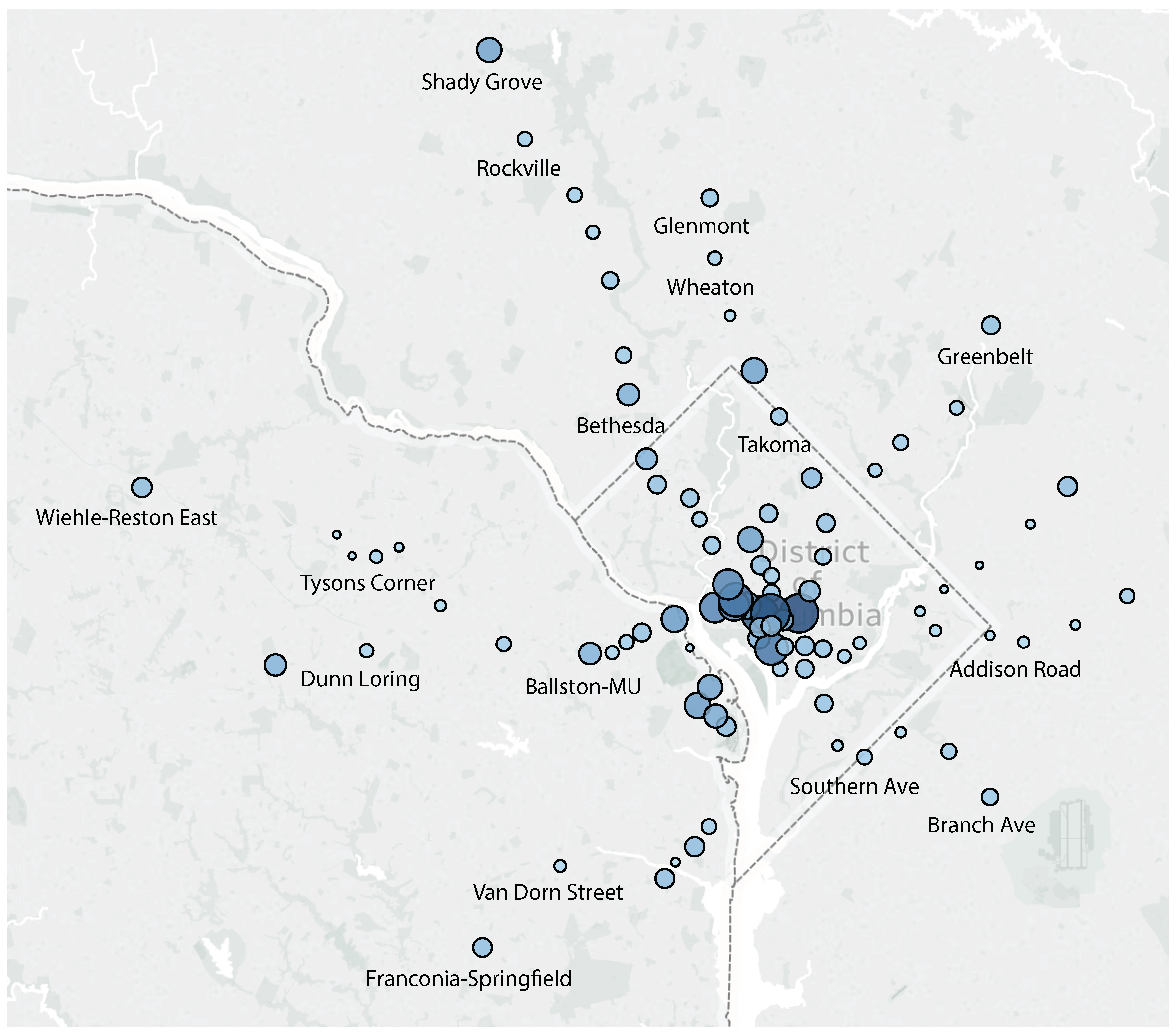
Our objective is to assess and predict passenger flow in public transportation systems. In our work, we use the metro system of Washington, DC as a case study. The Washington Metro has a total of six lines that cover the entire DC metro area, i.e., Washington, DC and parts of Maryland and Virginia. Those lines partially overlap in terms of the rail network they use. The network comprises a total of the 91 stations shown in Figure 1.
Data from fare card records was acquired from the Washington Metropolitan Area Transit Authority (WMATA). Each record in this dataset consist of four values: entry station, entry time, exit station, and exit time. Based on these records, on average, there are 600,000 trips per weekday, 200,000 trips on weekends, and a total of 14 million trips per month. Not all stations are equally busy. For illustration, reconsider Figure 1, which not only shows the station locations, but also its respective passenger volume (indicated by circle size and color). Larger circles of darker color represent more passenger traffic. For example, the busiest station during January 2017 was Union Station with 650,000 passengers beginning their trip at this station. In contrast, only 24,000 passengers entered the least frequented station, Cheverly, during the same time period.
We aggregated the passenger inflows and outflows at stations per 15 min intervals to construct time series of traffic volume per station. The passenger volume is not only station specific, but also time specific. Consider here the example of the Vienna station to the east of Washington, DC. Vienna is the most western Orange Line station, located at a residential area. It is a classical commuter station, i.e., people take the metro in the morning commuting towards the city center and return likewise in the afternoon. A typical weekday passenger volume graph for this station, observed on Wednesday, February 8, 2017, is shown in Figure 2a. A station located at the city center, such as Federal Triangle (cf. Figure 2b), shows a complementary flow, i.e., people exiting the station in the morning and entering it in the afternoon to return home. Figure 2c shows a somewhat different station, “Arlington Cemetery”, with people arriving and leaving throughout the day. Notice here the significantly lower passenger volume when compared to commuter stations, i.e., 30 vs. 600 passengers per peak 15 min interval (temporal granularity of graph). Observing these passenger volume fluctuations with respect to stations and time, our goal is now to assess and predict it.
4. Problem Definition
We formalize our database of passenger volume in the following:
Definition 1 (Passenger Flow Database).
Let denote a database of in- and outflow of passengers of a public transportation network Let denote the set of all n stations, and let be the set of days covered by this data set. For a given station and a given time , we let and denote the time series of passengers entering and, respectively exiting station on day .
As an example, the left of Figure 2a shows the inflow , while the right of Figure 2a depicts , i.e., the corresponding outflow.
To combine inflow and outflow, we let
denote the time-series obtained by concatenation of in- and outflow for station i on day j. For instance, is the notation of the concatenation of the two time series shown in Figure 2a, for the Vienna Station on February 8, 2017.
Furthermore, for and for a list of days we let
denote the concatenation of all time-series of station for days in T. In the same sense, we define the time-series of the overall flow of a list of stations S on day j as the concatenation:
Given a passenger flow database as defined above, the challenges approached in this work are to classify days and stations, and to predict future passenger flow. The problem of classification is, given the time-series of a day at a station, to infer the unknown station name and day. The problem of prediction is defined as follows.
Definition 2 (Passenger Traffic Prediction).
Let be a one-day station time series. Further, let be the known time-interval of Q on day . The task of passenger prediction is to predict the values of passenger flow during the unknown time of Q, given .
Both challenges will be addressed in the following two sections.
5. Methodology
In this section, we present our approach to model, classify and predict public transport traffic volume.
5.1. Feature Extraction
As described in Section 4, passenger volume is given by time series of inflow and outflow at each station for each day. Thus, each station is represented by a high-dimensional feature vector , corresponding to inflow and outflow at station i over all days. For example, for the data dataset described in Section 3, each station is represented by a -dimensional (2 flow-directions times four quarters per hour time 24 h a day times 59 days) feature vector that corresponds to 15-min intervals of in- and outflow for the 59 days in January and February 2017. At the same time, each day j is described by a -dimensional feature vector . Even for a single (station, day)-pair, we have features in our dataset. Yet, clearly, the intrinsic dimensionality of these feature spaces is much lower since some features contain no information, while others are highly correlated. Consider here that the metro is closed between the hours of 02:00 and 05:00 and the passenger volume is 0. Further, many stations and/or days exhibit very similar passenger volumes.
Thus, to obtain a more concise volume representation of each (station, day)-pair, we reduce these d-dimensional feature spaces to a dimensional space using Principal Component Analysis (PCA) [23]. Although we cannot interpret these latent features directly (as they are linear combinations of the non-reduced d-dimensional features), we can benefit from the fact that PCA maintains similarity between features. Thus, two days (or two stations) that are similar in the full dimensional feature space, are likely to remain similar in the reduced feature space.
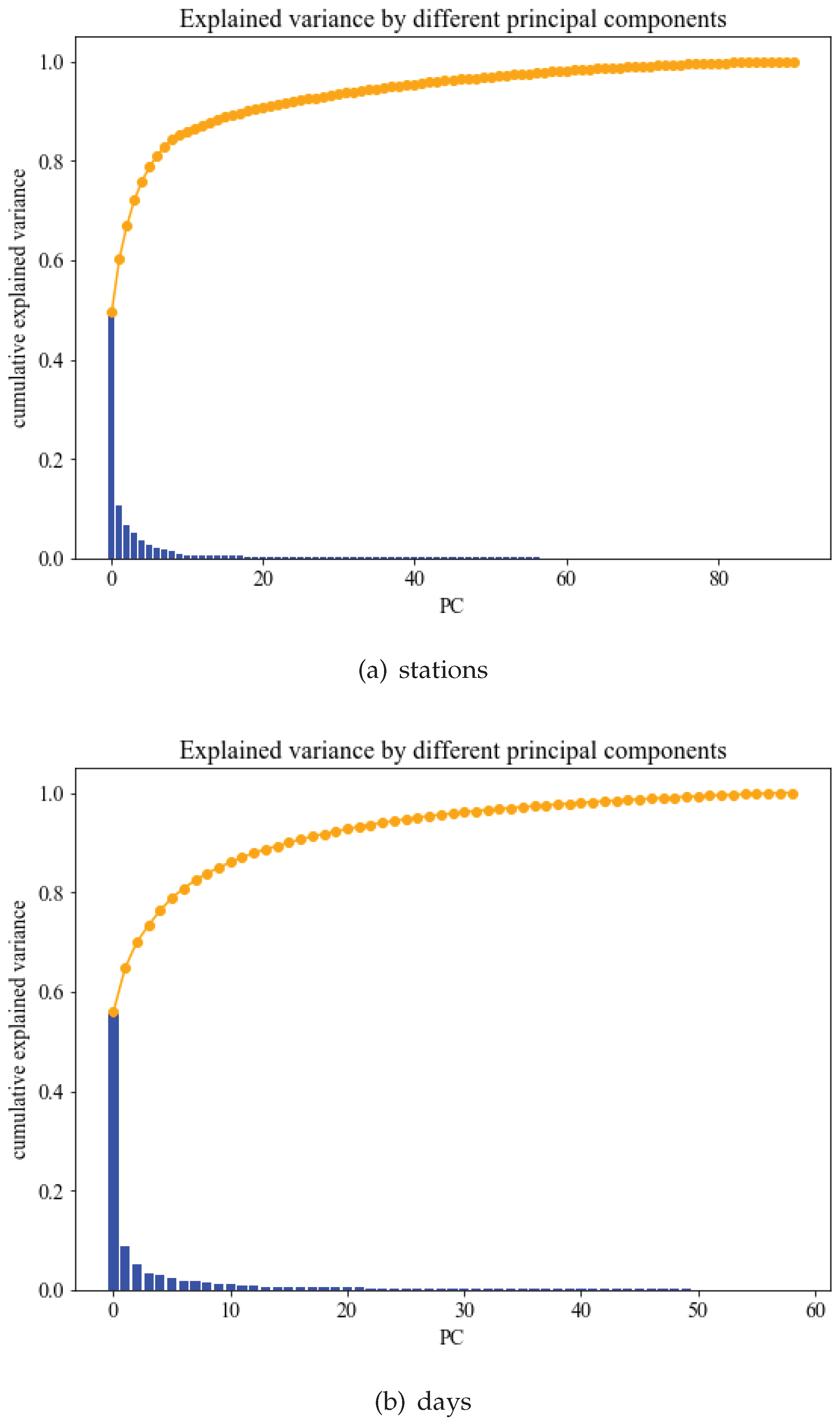
Figure 3a shows the cumulative explained variance for the maximal set of principal components from the PCA on the data per station. The blue boxes show the explained variance per component. As can be observed, for the cumulative explained variance is already above 80%. For our evaluation, we use latent features as default, which preserve 85.24% of the original data variance. Figure 3b shows the corresponding variance graph for the principal component analysis of the data per day. We observe a similar behavior and choose with a cumulative variance of 84.95%. We denote this K-feature PCA-representation of a time series as . The next section shows how we utilize the reduced time series representation to cluster similar stations and similar days.
5.2. Unsupervised Labeling of Stations and Days
Once time series have been transformed into a lower dimensional feature space using PCA, we can cluster similar days and train stations. To identify similar stations, we cluster the latent features of inflow and outflow of all stations over the full time horizon . For this purpose we use hierarchical agglomerative clustering, often used to cluster features of high-dimensional data such as text [24,25] using the single-link distance to merge clusters in each iteration. This approach yields a cluster dendrogram, which we can analyze visually to identify the number k of meaningful clusters. Using k, we cluster the latent feature space using k-means [26]. We use the same approach to cluster the latent features of all days to find groups of similar days. Our proof of concept in Section 7 provides dendrograms based on the Washington, DC metro passenger volume, which show that the PCA features do indeed allow to group semantically similar metro stations. For this dataset, our clustering approach allows to automatically group (i) days into weekdays and weekends, and (ii) stations into commercial, residential, mixed, but also downtown and suburban.
5.3. Classification
The time series of the passenger flow at each station, after it is transformed to a lower dimensional feature space by PCA, is assigned with a label that corresponds to (i) the station id or (ii) the cluster id, provided by the clustering of stations that was performed using the latent features derived from PCA, as described above. We approach the challenge of automatically identifying the unknown station of an unlabeled time series , thus mapping to a station in . We approach this problem on multiple levels of difficulty:
- Task I: Classifying the type of a station, using the unsupervised grouping of stations into clusters as described in Section 7.2.
- Task II: Classifying the exact station label.
Clearly, Task I is the easier task, as it is a k-class classification problem, where k is the number of station clusters that we obtained in Section 7.2. In contrast, Task II is a -class classification problem. In particular, some stations may have very similar inflow and outflow throughout the day. For Task I, the challenge is merely to identify the unknown station as “one of these”, rather than mapping to the exact station. For example, in our Washington, DC metro farecard data set, we have a total of 91 stations, while having only five station types.
We achieve this classification by using a lazy m-nearest neighbor classification using as the query in the latent feature space of all (station, day)-pairs available for training. The result is a set of m feature vectors from the training set for which stations and days are known. We use the distance-weighted majority vote to classify the station and day of Q.
Example 1.
Given a timeseries , observed on March 8, for which inflow and outflow are known, but the station label is unknown. Transforming the feature transform , using a -nearest neighbor search, we find the five most similar reduced time series , , , , and . In this result, three 5 nearest neighbors are labelled with , one neighbor is labelled with , and one neighbor is labelled with . Using the majority vote, we classify as to solve Task II. For Task I, we first check the type of each station, and return the majority of their types.
5.4. Prediction
The main contribution of this work is to predict the passenger volume of a station, using the tools defined in Section 5.1, Section 5.2, Section 5.3, Section 5.4, Section 6, Section 6.1, Section 6.2, Section 7, Section 7.1 and Section 7.2. At a given point in time, and for a given station Q, we want to use past passenger volume to predict the future volume. For example, we may want to predict the volume of a station in the afternoon, based on the volume before noon. To perform this prediction, we use an approach similar to the classification approach in Section 5.3. We first find similar (station, day)-time-series of similar volume trends (in terms of latent features) to Q before a given point in time, in order to use their volume after that point in time, as a prediction. In particular, we map all time series in to the (known) past time interval , yielding the database . Then, we perform a kNN-classification on the latent feature space using only information of the time interval of the whole database. The result is a set of k trajectories having the most similar latent features to Q during time interval . For these trajectories, the unknown time interval is averaged and used to predict Q.
6. Proof of Concept
With this initial proof of concept, our goal is to find similar stations and days in terms of passenger volume. As such we apply the clustering described in Section 5.2 and discuss the results in the following.
6.1. Clustering of Stations
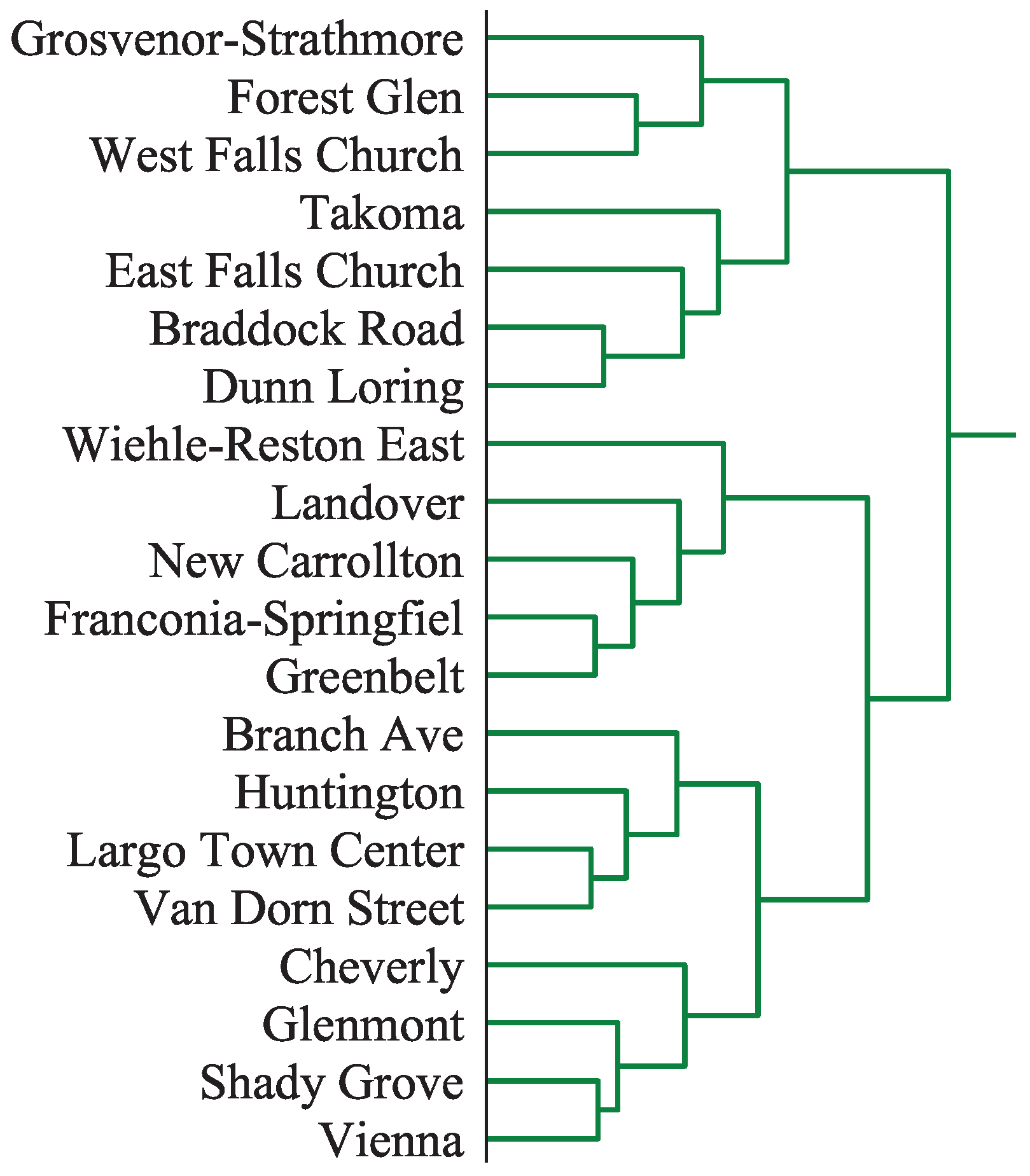
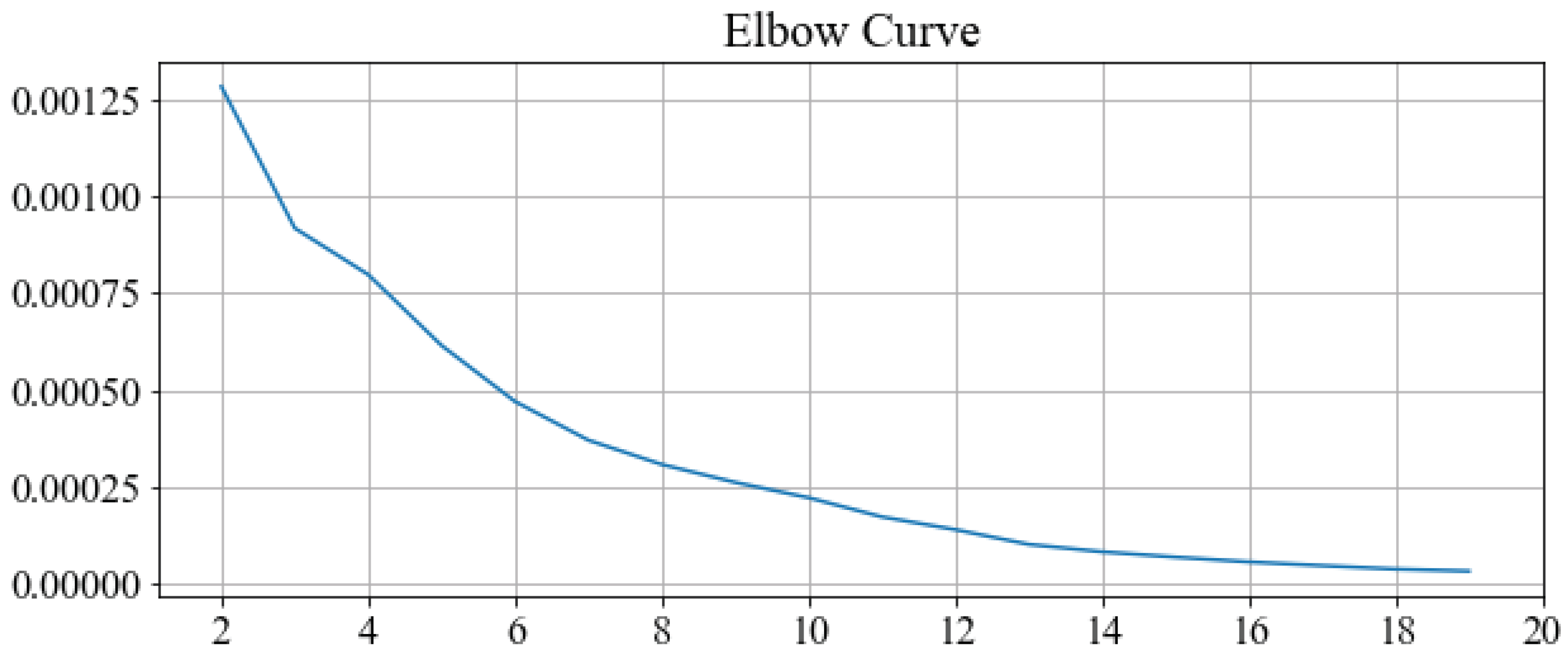
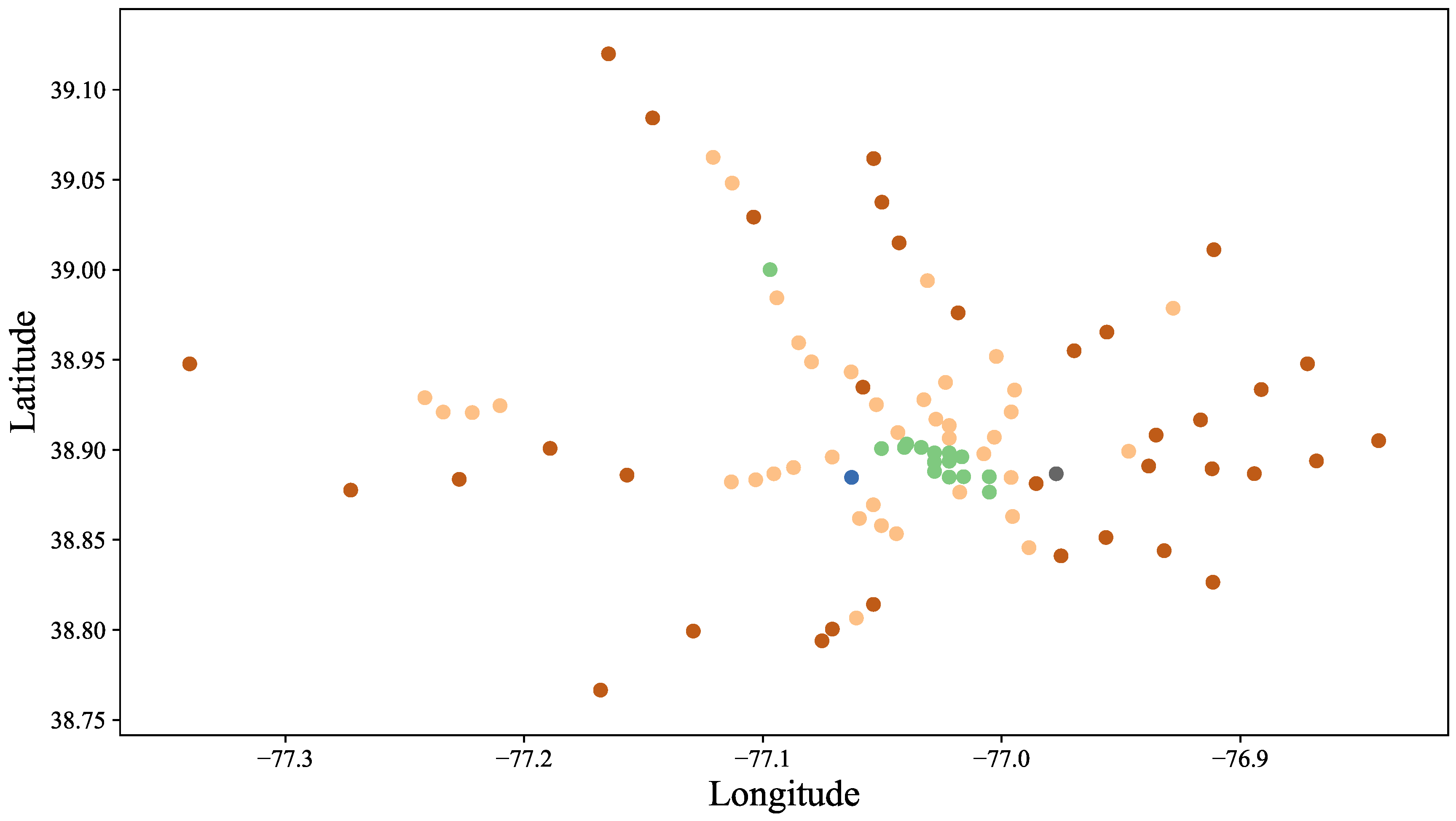
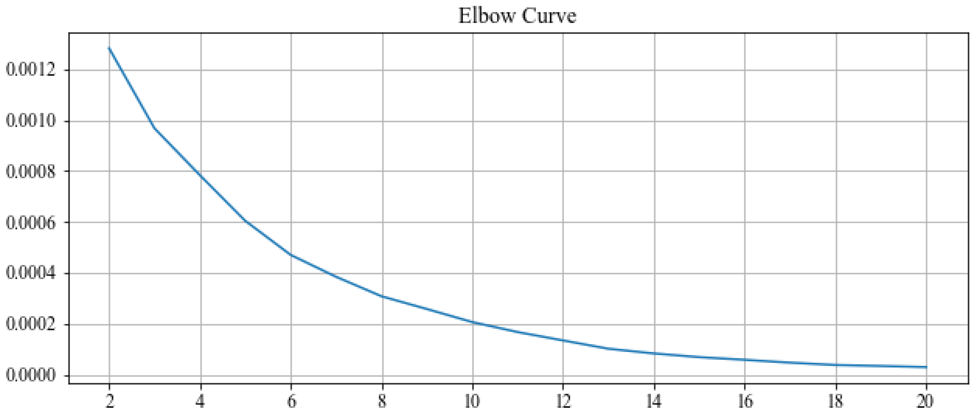
A part of the single-link dendrogram for clustering the latent features of the 91 stations in the Washington, DC dataset, as described in Section 4, is shown in Figure 4. The full dendrogram of all 91 stations was not included, due to space limitations. It showed that the latent features of train stations exhibit large groups of mutually similar stations, with only a few outliers. Additionally, Figure 5 shows the elbow curve where we vary number of clusters from 2 to 20 and plot the corresponding sum of squared distances of points to their closest cluster center. There is a very small elbow for k = 3, however, distortion is still high. Choosing clusters, and running k-means on the set of all stations, yields the clustering shown in Figure 6. We can clearly observe that the stations in the center of Washington, DC belong to the same cluster, thus exhibiting similar latent features. During weekdays, commuters exit these stations to reach their workplace in the morning and enter them in the afternoon to return home. While this cluster covers all stations in the downtown area (federal government buildings), there is one other station that belongs to this cluster. “Medical Center” is located approximately 10 miles to the Northwest of downtown and serves almost exclusively the National Institute of Health (NIH), which is another federal agency. The vast majority of passengers at this station are NIH employees/visitors and as such the station has a similar profile to the downtown area.
Another characteristic cluster is that of suburban stations which create a characteristic ring around Washington, DC (shown in dark red color). These stations mostly serve suburban residential areas. Passengers at these stations typically are commuters that take the metro to get to work in the morning and to return home in the afternoon.
A third characteristic cluster is the inner ring of stations around DC (depicted as orange dots in the figure), which serves mixed (residential and business) areas. At these stations, incoming and outgoing passenger volume peaks in the morning as well as afternoon (“camel back” pattern).
We also observe two very interesting outliers, which are dissimilar to any of these clusters. One outlier is “Arlington Cemetery”. With no residential or business traffic, its passenger volume is dictated by funeral services and tourism. The second outlier is “Stadium Armory”, which serves the RFK soccer stadium. Since there are no games during winter, this station is expected to have very little passenger volume as recorded in our datasets for January and February of 2017.
Overall, clustering the stations based on passenger volume revealed characteristic concentric ring-shaped clusters of stations. An outer ring captures stations serving suburban residential areas. Passengers commute from there to business district stations downtown (center cluster). In between are stations that serve mixed areas that include residential as well as business areas (inner ring).
6.2. Clustering of Days
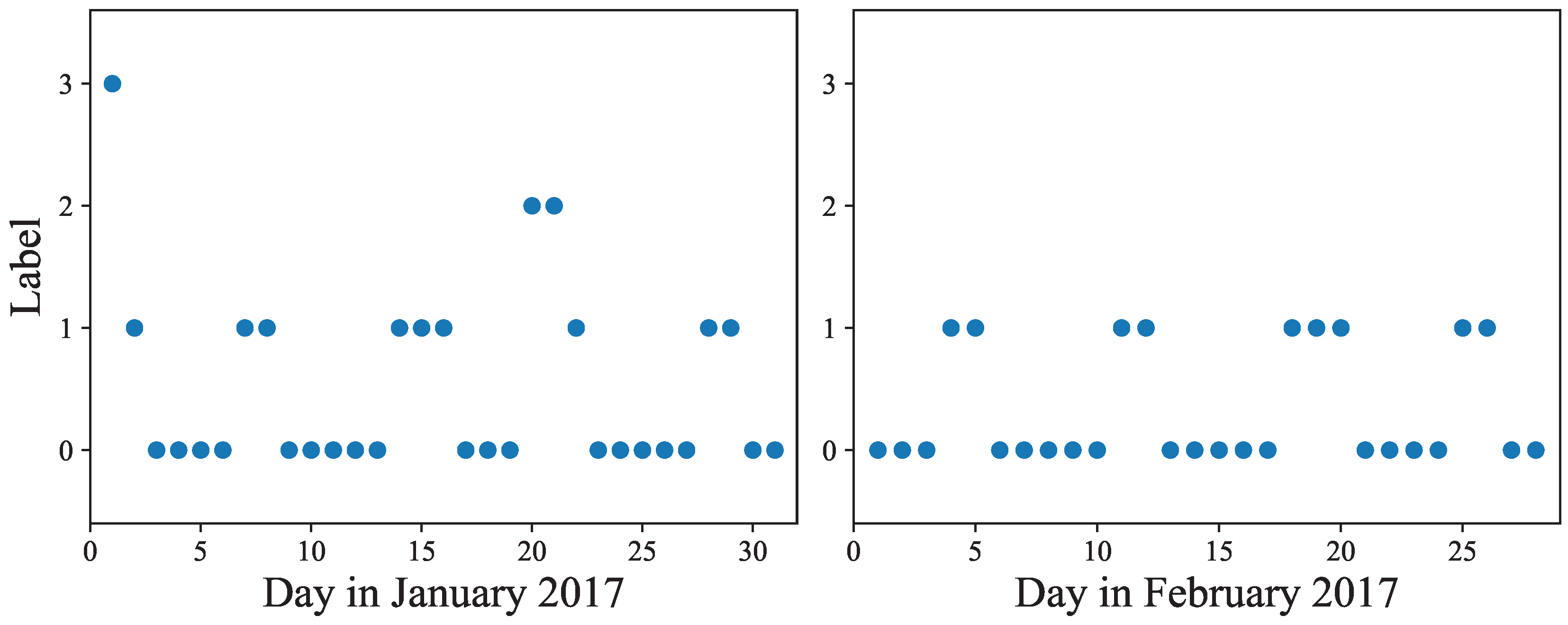
Following the elbow method to determine a useful number of clusters, we present the decrease of the sum of squared distances of samples to their closest cluster center, as we increase k from 2 to 20 clusters in Figure 7. No clear elbow can be seen. We choose k = 4, expecting to see the categories of weekdays, weekends and a few special days or outliers. Figure 8 shows the result of running a 4-means clustering on the latent features of the days of January and February 2017. We see that weekends and holidays were perfectly grouped together, keeping in mind that Monday, January 2 was the observed ‘New Year’s Day’, Monday, January 16 was a federal holiday (Martin Luther King Day), and Monday, February 20 was President’s Day, another federal holiday. Normal week days perfectly fit into the other clusters.There are two outliers which constitute their own cluster: January 20 and January 21, Inauguration Day and the day of the Women’s march, respectively. Both days had unusual event specific passenger volumes and some stations were closed. This shows that the latent features of our passenger volume data can be used to distinguish between days of the week and weekends, and to detect ‘special’ days such as holidays.
Overall, the results of this section prove our concept, that the information stored in our database , even after the reduction to latent features, allows to discriminate different days and different stations as well.
7. Experiments
The clustering of days and stations in Section 6 showed that the latent feature space of passenger volume time series is highly discriminative. We can identify similar stations and similar days in a semantically meaningful way. The following sections will now show how a classification of days and stations (cf. Section 5.3) yields high classification accuracy, and how our approach to predicting passenger flow (cf. Section 5.4) significantly outperforms the naïve solutions of relying on daily and weekly periodicity patterns.
7.1. Data
The metro dataset that we use for our evaluation includes all 91 stations from the DC Metro network. It contains data from January 1, 2017 to February 28, 2017. Each record consists of the station name and timestamp from when an anonymous passenger entered the Metro system, as well as the station name and timestamp from when the same passenger exited the system. We aggregated the incoming and the outgoing passengers of each station per 15 intervals, to form inflow and outflow histograms per station per day.
7.2. Classification
Our first set of experiments addresses train station classification. We employ a leave-one-out cross validation, thus querying the feature representation of both in- and outflow for each station and day , and finding its nearest neighbors in the set of latent feature vectors . For comparison, we also used a Multi-Layer Perceptron (MLP) classifier, a feedforward neural network with a hidden layer of 100 neurons, a logistic activation function and an adam solver. We used the implementation of the scikit-learn python package [27].
7.2.1. Number of Nearest Neighbors
We first perform an experiment to assess the best value of k of the kNN classifier for our analysis. To this end, we vary the number of nearest neighbors from 2 to 30. The results of this experiment are shown in Figure 9, grouped by days. For each day, the plotted accuracy corresponds to the number of correctly identified train stations. As can be observed, for many weekdays the classification accuracy is very high, at least 90%, and there is a tie among the different values of k in these cases. However, for the days in which the classification accuracy is lower, we can observe that k = 5 is a reasonable choice as it achieves the highest accuracy in many cases.
7.2.2. Classification Accuracy
Having chosen k = 5, we compare our latent feature based 5NN classification to the MLP classifier and present the results in Figure 10a. We observe that both methods yield comparable classification accuracy results. On about a third of the days, the kNN classification marginally outperforms the MLP, while for the remaining cases the reverse holds. Nonetheless, both results are very similar. We observe that most of the weekdays show a or higher accuracy, implying that the vast majority of train stations was identified correctly for those days. This accuracy drops to about for most weekend days, implying that weekends show a higher variability in terms of passenger flow. Furthermore, we have fewer weekend days than weekdays, such that some of the lower accuracy can be attributed to having fewer training instances. We also note a poor accuracy on January 1, a day that is untypical due to the new years celebrations, as well as Inauguration Day on January 20 and the Women’s March on January 21. The similar effect of those days on clustering has been explained in Section 6.
Furthermore, we observe a lower accuracy for February 4 and February 5, which was initially surprising. However, further research on metro operations revealed that several stations were closed for maintenance. The last outlier is Sunday, January 8, a day on which only five out of 91 stations were classified correctly. We attribute this low accuracy to the lowest observed passenger volume (by far) on this day in our entire dataset. Only 108,000 passengers frequented the metro on this day, while the next lowest volume was 170,000 passengers (another Sunday), and most weekdays have upwards of 600,000 passengers. Over all the days, the average precision of 5NN was approximately , which is a strong result considering that this is a 91-class classification problem, where random guessing would yield an expected accuracy of less than .
The task of classifying the type of station is easier, as explained in Section 5.3. Thus, the classification based on the five cluster labels of Figure 6 yields a much higher accuracy. The results of this analysis are reported in Figure 10b. Similarly to the previous experiment, both kNN and MLP classifiers yield similar results, with MLP having a slight advantage on some of the days. On many weekdays the classification accuracy reaches its highest at . Even for the outlier on Sunday, January 8, half (45 out of 91) of the stations were classified as their correct type by 5NN, yielding a accuracy, versus by the MLP. This result is still better than the expected accuracy of random guessing of one out of the five cluster labels. The overall accuracy of this task for all the days was .
7.3. Prediction
In our final set of experiments, we forecast, for each day and each station, the 48 dimensional time series past noon, given the 48-dimensional time series before noon. We perform a leave-one-out cross validation. In other words, we consider each (station, day)-pair individually as the test set, and use all the remaining station data for training (cf. Section 5.4). We employ a kNN regressor trained on the latent features that we extract using PCA on the prior to noon time series of each station-day pair. While we use the five nearest neighbors in the following, we note that we also experimented with varying values of k = 2,3,5,10,20,30. The resulting predictions were of almost identical quality in terms of average absolute errors. For this reason, we only report the 5NN prediction results. We compare the latent feature based approach to that of artificial neural networks. In particular, we use the Multi-Layer Perceptron (MLP) regressor, a feedforward neural network with a hidden layer of 100 neurons, a logistic activation function and an adam solver. We used the implementation of the scikit-learn python package [27]. In the following experiments, the MLP receives the original features as input, while the kNN regressor operates on the latent features. We also include two naïve baseline prediction methods, we use the time series of the same station from the previous day (Daily Periodicity) and that of the previous week (Weekly Periodicity). In the first week, with no data available for the weekly periodicity approach from the previous week, we use the second week for prediction. The same applies for the first day of the daily periodicity prediction. To measure the absolute prediction error, we use the Euclidean distance between the predicted time-series and the ground-truth time series.
7.3.1. MLP Settings
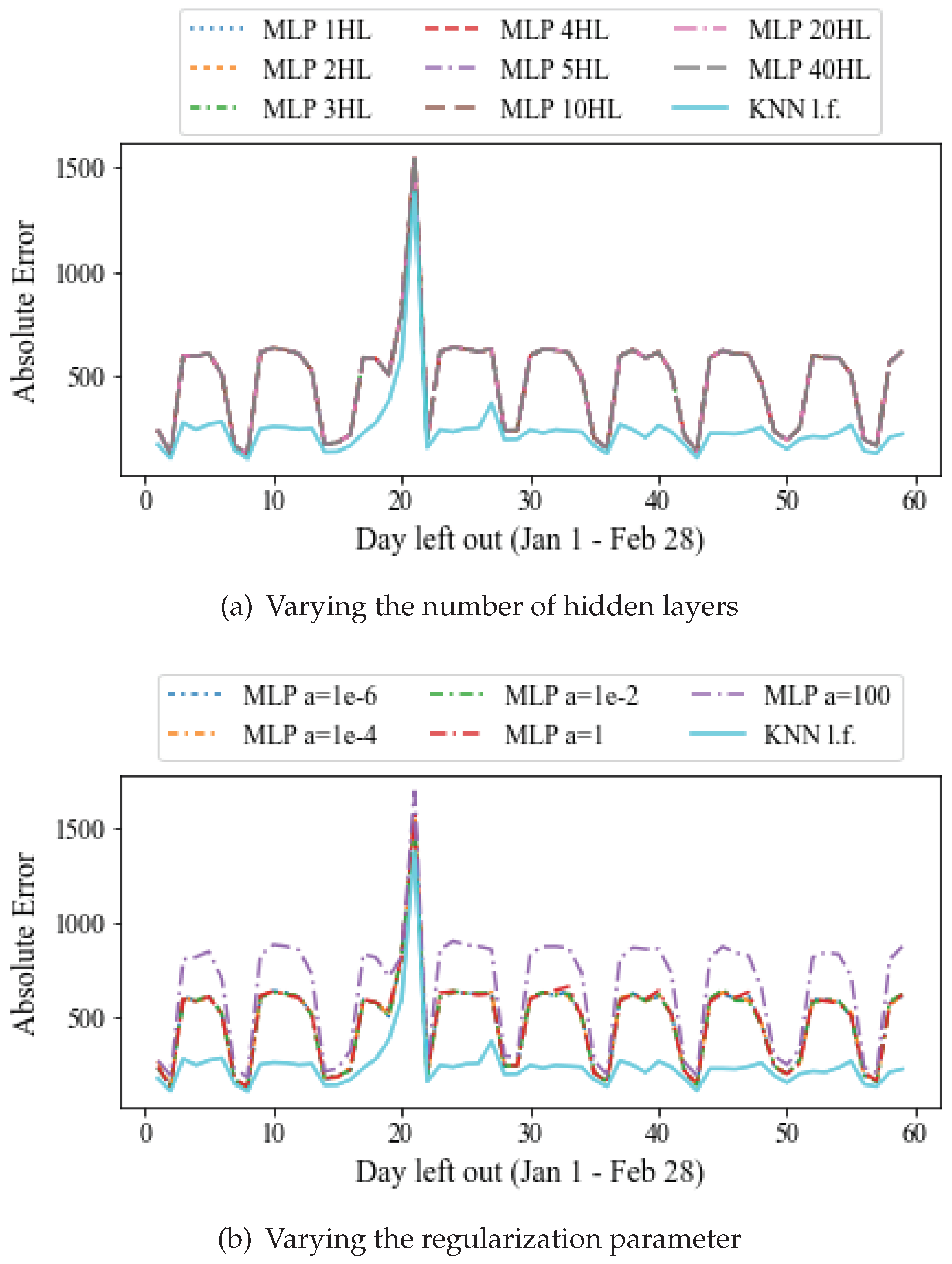
Figure 11 shows the absolute prediction error averaged for all 91 stations, for varying settings of the MLP regressor. In Figure 11a we vary the number of hidden layers from 2 to 40. Each layer consists of 100 neurons by default. It can be observed that the average prediction error is almost insensitive to the number of layers of the network. This error is always larger than the latent feature based approach. The reason for this may be that the size of the dataset is not adequate for the training of a neural network, which typically performs better on larger datasets. The execution time increases monotonically with the number of layers, while the prediction quality remains constant. Therefore, in the remaining experiments we choose 1 hidden layer by default.
Figure 11b shows the absolute error averaged for all 91 stations, for different values of the parameter a. This parameter is for regularization (penalty) term, that combats overfitting by constraining the size of the weights. Increasing a may fix high variance (a sign of overfitting) by encouraging smaller weights, resulting in a decision boundary plot that appears with lesser curvatures. Similarly, decreasing a may fix high bias (a sign of underfitting) by encouraging larger weights (http://scikit-learn.org/stable/auto_examples/neural_networks/plot_mlp_alpha.html) [27]. It can be observed that increasing a to 100 can lead to higher prediction errors. On the other hand, for a between and 1 the MLP errors remain almost the same. The computational cost does not vary significantly with a in our experiments. Thus, we choose the default parameter of , which is also the predefined value by the scikit-learn implementation.
7.3.2. Prediction Quality
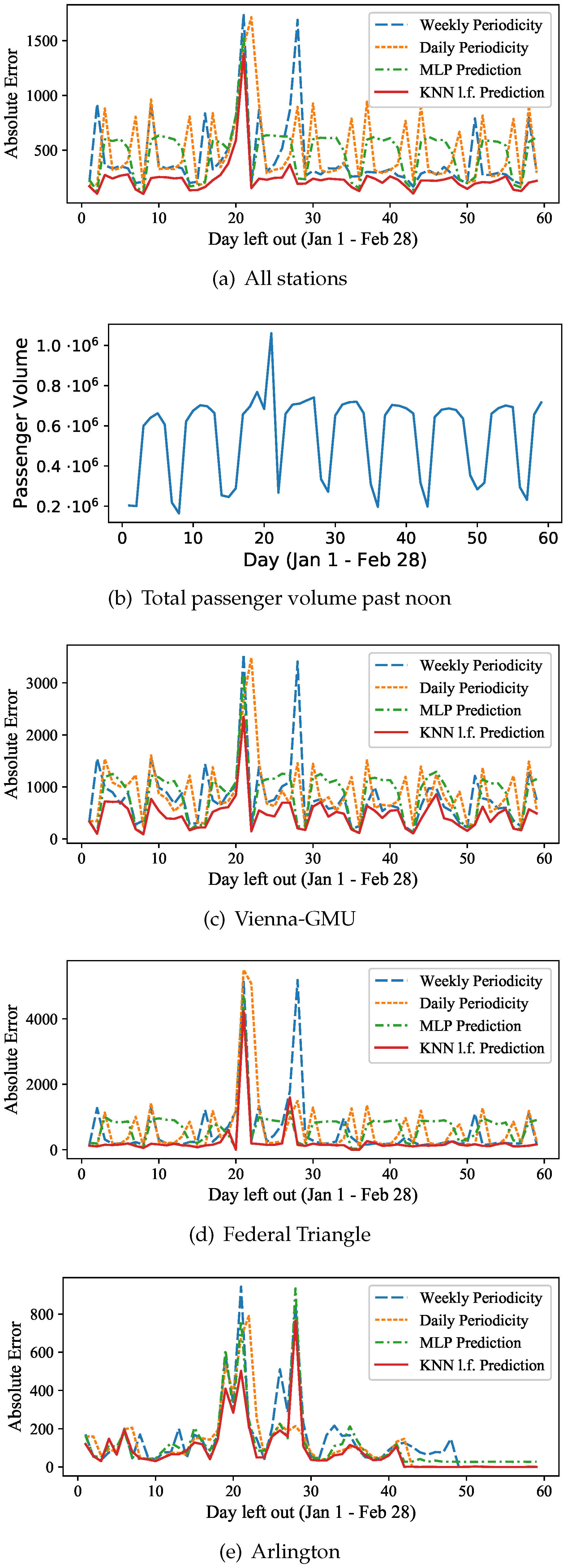
A more detailed comparison of the prediction results is shown in Figure 12 and Figure 13 which includes the Daily Periodicity approach, the Weekly Periodicity approach, the MLP neural network, and the latent feature based kNN approach. In the first graph of Figure 12a, for each day, the prediction error is averaged for all 91 stations. For reference, the total passenger volume that passed from all stations each day after noon is shown in the next graph of Figure 12b. We immediately observe substantial errors for January 20 and January 21, which are Inauguration Day and the Women’s March, respectively. Clearly, these events were non-periodic and thus difficult to predict. The Weekly Periodicity also exhibits a large error seven days after these events, which is expected, as it simply uses the previous week for prediction, and thus expects an Inauguration and Women’s March type event to occur. For the Daily Periodicity, this behavior is observed on the next day, January 22. Both the latent feature based kNN prediction and the MLP prediction results observe high errors on January 20 and January 21, without these two events affecting the prediction quality of other days. The latent feature kNN approach, however, is more resilient and has a lower error than any other approach on those two days, as well as on the remaining of the ‘normal’ days of our time series. The MLP absolute error follows a similar behavior as the curve of the total aggregate passenger volume of Figure 12b, and reaches up to 700 out of about 7 passengers on ‘normal’ weekdays. The latent feature based kNN prediction maintains errors below 300 passengers (about 0.004% of the total passenger flow) on most typical weekdays.
Figure 12c–e show the prediction errors for three individual stations: Vienna-GMU (suburban), Federal Triangle (central) and Arlington Cemetery (outlier). The first two have higher absolute errors as they also have significantly larger passenger volumes than Arlington station. The Federal Triangle is located at the center of D.C. and has lower errors on most days, except for Inauguration Day and the Women’s March, where the kNN prediction still outperforms both the neural network (MLP) as well as the periodicity-based approaches. Other than the two outliers, the latent feature based kNN method gives near-zero prediction error for most of the remaining days. This is expected, as the behavior of passengers should be easier to predict on normal days at a central station that commuters visit daily to go to work. A similar behavior can be observed for Vienna-GMU, a suburban station that residents commute from to get to work. Arlington Cemetery on the other hand has more varying prediction errors. They are higher (400–800 passengers) on the week of January 19–25, while the Weekly Periodicity prediction gives high errors for the next week as well. For all three stations, the latent feature based kNN prediction method demonstrates lower errors than employing a basic artificial neural network (MLP) or simply relying on the Daily or Weekly Periodicity.
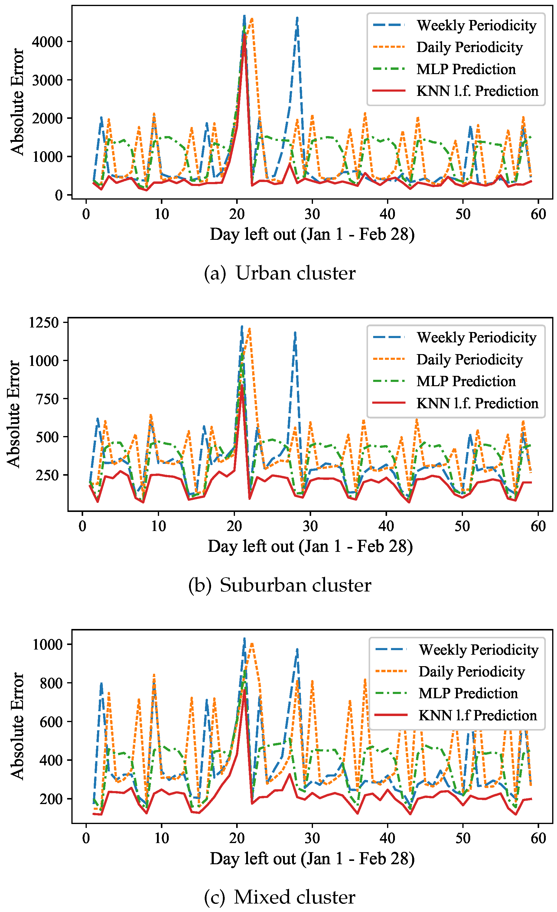
In the Figure 13a–c we present the absolute prediction errors, averaged over the stations that consist each of the three major clusters of the 5-means, as shown in Figure 6. These are the urban cluster (green central stations), the suburban cluster (dark red outer ring) and the mixed clusters (yellow inner ring). In all these experiments, the latent feature based kNN approach outperforms the daily and weekly periodicity predictions, as well as the MLP prediction. For the stations that belong to the urban cluster, located mostly at the city center, even on “normal” days (i.e., excluding the outliers of 1/20 and 1/21) the average prediction error may exceed 2000 passengers on some days for the weekly and daily periodicity, while it always remains below 600 for the latent feature based kNN approach. On these typical weekdays, the prediction error of the MLP is on average up to four times higher than that of the latent feature based prediction. A similar behavior can be observed for the suburban cluster on Figure 13b, but the average absolute errors are generally lower (below 1250) for all dates and methods. The MLP again fail to outperform kNN on typical weekdays, having about double the prediction error. The mixed cluster contains stations in areas that can be both for business and residential. Both the weekly and the daily periodicity prediction introduce high errors (peaks are between 600 and 1000 passengers) on many dates, the MLP errors are of more than 400 passengers even on normal weekdays and peak on 900 passengers for the outlier days, while the latent feature based kNN prediction remains low, below 300 passengers, on all normal days, and it is 20% better on the two outlier days.
7.3.3. Relative Gain in Error
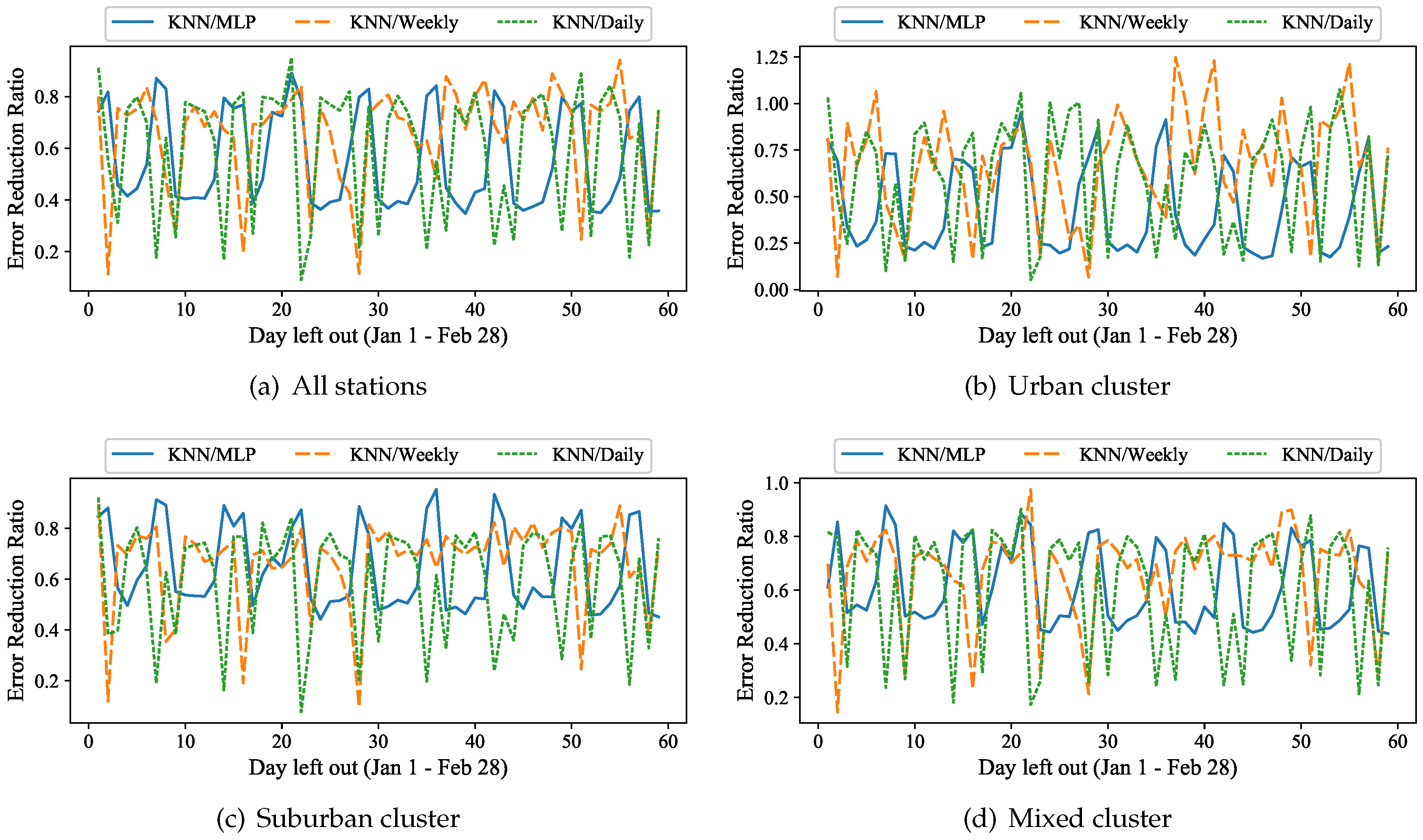
Overall, we see that our examined kNN passenger flow prediction, using expressive latent features, significantly outperforms the naïve periodicity approaches and is consistently better than the MLP neural network prediction. It yields better prediction results for every single day and significantly outperforms these approaches for many days. To better illustrate this gain, Figure 14a shows the relative reduction in prediction error, i.e., the ratio of the absolute prediction error of the latent feature based approach to the MLP error as well as the weekly and to the daily periodicity prediction errors, averaged over all the stations. For most weekdays, the error is reduced by only about of the weekly periodicity prediction. Given the fact that most weekdays have similar passenger flow, such a moderate improvement is expected, i.e., simply using the periodic data from the week before results in most cases in an acceptable prediction. Still, we want to stress that our approach is able to significantly improve the prediction for such “typical” days and for which the previous week should be a good forecast. We explain this improvement by the ability of our approach to learn latent, unobservable features such as the weather. Even though our data does not explicitly capture any weather information, our approach is able to learn such latent features. It may for example decide that the first 12 h of the day to be predicted look like “a rainy Wednesday”, and thus, it may not choose the previous Wednesday, but another rainy weekday as a template for the afternoons’ passenger volume prediction.
Daily periodicity prediction typically suffers on Saturdays and on Mondays, as it tries to predict the behavior of a weekend day using a weekday (i.e., uses the passenger volume of Fridays to predict the volume of Saturdays), and vice versa (i.e., using the passenger volume of Sundays to predict Mondays). In those cases, our approach improves the prediction by 60–95%.
In addition to the already significant improvement in prediction accuracy, compared to the periodicity based approaches, our approach really shines on weekends, which show a more irregular behavior. For many weekend days and holidays, our approach shows a 70–95% reduction in prediction error of the weekly periodicity. We contribute this highly relevant result to the fact that weekends are less periodic, and more susceptible to latent factors such as temperature and weather. People have to go to work regardless of these latent features, but on weekends, their travel might be more influenced by bad weather, i.e., they stay home when it rains.
Contrarily to the periodicity based approaches, the MLP prediction suffers more on the most typical weekdays, when it tends to underestimate the true passenger volume. The latent feature based outperforms the MLP on all days. However, on these typical weekdays, our approach is able to achieve 2.5 times less error on average over all stations, compared to the average absolute error of the MLP.
Examining the groups of stations that fall in each of the three major clusters of the 5-means separately, we can observe a relatively similar behavior as described above for the full set of stations. Figure 14b shows the relative reduction in prediction error only for those stations that belong to the urban cluster. Our approach outperforms the two baselines, with only two exceptions: Monday, February 6 and Friday, February 10, where the weekly periodicity gives 25% and 23% better results, respectively. On both those dates, however, the relative errors of both approaches are already below 0.054 and below 0.044, respectively. In terms of the MLP, the gain of the latent feature-based approach is more evident for the results of the urban cluster. Our approach outperforms the MLP on every day. It achieves on average 25% lower errors on the weekends, while it achieves a four times higher prediction quality than the MLP over the weekdays. Furthermore, our method outperforms the periodicity-based approaches as well as the neural network prediction (MLP) on every single date for both the suburban and mixed clusters of stations, as shown in Figure 14c,d.
7.3.4. Computational Cost
In terms of computational cost, we measured the average execution time over 100 runs of our method, as well as the weekly and daily periodicity prediction baselines. All the experiments were performed on an Intel Core i5 2.2GHz CPU computer with 11.4GB RAM, running Ubuntu Linux. Both methods were implemented in Python. As expected, the two periodicity-based approaches were faster, with an average of 0.029993 s. The MLP prediction was slower, requiring an average of 14.752 s for a neural network with one hidden layer, while it required up to 260.58 s on average for 40 hidden layers. Our proposed latent feature-based method required an average of 2.284 s, which is not surprising as it searches the entire space of possible (station, day)-pairs, instead of only looking at the same time on the previous day or at the same day and time last week.
8. Conclusions
This work focuses on modeling and predicting passenger volume in public transport systems based on mining fare card log files from the Washington, DC Metro system. By using a latent feature analysis approach, we were able to show that time-series of passenger in- and outflows at stations are highly discriminative, allowing us to distinguish different stations as well as weekdays with extremely high accuracy. Using two months of passenger volume data for 91 stations, our evaluation shows that individual stations can be identified with high accuracy. Further, our approach of predicting passenger volume at stations is highly effective and outperforms the two naïve baselines of daily and weekly periodicity prediction, as well as an MLP neural network for every single day. The prediction accuracy improvement was high in many cases as demonstrated by our results.
One of the limitations of our analysis is that we were only given access to completely anonymous fare card data. Thus we were only able to work with aggregates of passenger volume over time. Had we been given pseudonymized data, i.e., pseudo-ids associated with metro users’ records entering and exiting the metro system at specific stations and times, then we would be able to perform a more in-depth analysis of the passenger flow patterns over time and extend our work to passenger profiling. We see this as a direction of future work. Another limitation of our analysis is that our dataset spans over the period of two months. Given larger datasets, spanning over longer periods of time, we may have been able to employ deep learning and effectively train multi-layer neural networks in the prediction of passenger flow in the examined metro network and achieve more accurate results. The low data availability gives an advantage to our latent feature-based approach compared to the neural network prediction. It remains to be examined in a future empirical study, whether this advantage continues to hold when dealing with significantly larger data sets. However, it is typically hard to obtain the aforementioned data; in the former case due to passenger privacy issues, and in the latter case due to public safety concerns.
Based on this work, we can give several directions for future research. Our overall objective is to determine human mobility volume, i.e., the flow of people over time and per area. As such, our approach is not only conceptually similar to traffic assessment on road networks, but also complementary, i.e., if we could combine the two volumes over time, it would give us an indication of how many people are present in, for example, different parts of a city. By combining even more movement sources, our goal is to create a movement model for urban areas, which can be used in a variety of application contexts such as emergency management, city planning, transportation planning or even geomarketing.
Author Contributions
Conceptualization, O.G., D.P. and A.Z.; Methodology, R.T, O.G., D.P., A.Z.; Software, R.T. and O.G.; Validation, R.T. and O.G.; Formal Analysis, A.Z.; Investigation, R.T.; Resources, D.P.; Data Curation, R.T. and O.G.; Writing—Original Draft Preparation, O.G., D.P. and A.Z.; Writing—Review & Editing, O.G., D.P. and A.Z.; Visualization, R.T. and O.G.; Supervision, O.G., D.P. and A.Z.; Project Administration, D.P.; Funding Acquisition, D.P. and A.Z.
Funding
This research was funded by the National Science Foundation AitF grant CCF-1637541.
Conflicts of Interest
The authors declare no conflict of interest.
References
- Metro Facts 2017. Available online: https://www.wmata.com/about/upload/Metro-Facts-2017-FINAL.pdf (accessed on 26 July 2018).
- Pelletier, M.-P.; Trépanier, M.; Morency, C. Smart card data use in public transit: A literature review. Transport. Res. Part C 2011, 19, 557–568. [Google Scholar] [CrossRef]
- Jolliffe, I. Principal component analysis. In International Encyclopedia of Statistical Science; Springer: Berlin/Heidelberg, Germany, 2011; pp. 1094–1096. [Google Scholar]
- Luo, D.; Cats, O.; van Lint, H. Analysis of network-wide transit passenger flows based on principal component analysis. In Proceedings of the 2017 5th IEEE International Conference on Models and Technologies for Intelligent Transportation Systems (MT-ITS), Naples, Italy, 26–28 June 2017; pp. 744–749. [Google Scholar]
- Zhong, C.; Manley, E.; Arisona, S.M.; Batty, M.; Schmitt, G. Measuring variability of mobility patterns from multiday smart-card data. J. Comput. Sci. 2015, 9, 125–130. [Google Scholar] [CrossRef]
- Roth, C.; Kang, S.M.; Batty, M.; Barthélemy, M. Structure of urban movements: Polycentric activity and entangled hierarchical flows. PLoS ONE 2011, 6, e15923. [Google Scholar] [CrossRef] [PubMed]
- Cats, O.; Wang, Q.; Zhao, Y. Identification and classification of public transport activity centres in Stockholm using passenger flows data. J. Transp. Geogr. 2015, 48, 10–22. [Google Scholar] [CrossRef]
- Toqué, F.; Khouadjia, M.; Come, E.; Trepanier, M.; Oukhellou, L. Short & long term forecasting of multimodal transport passenger flows with machine learning methods. In Proceedings of the 2017 IEEE 20th International Conference on Intelligent Transportation Systems (ITSC), Yokohama, Japan, 16–19 October 2017; pp. 560–566. [Google Scholar]
- Dou, M.; He, T.; Yin, H.; Zhou, X.; Chen, Z.; Luo, B. Predicting passengers in public transportation using smart card data. ADC 2015, 28–40. [Google Scholar] [CrossRef]
- Kieu, L.M.; Bhaskar, A.; Chung, E. Passenger segmentation using smart card data. IEEE Trans. Intell. Transp. Syst. 2015, 16, 1537–1548. [Google Scholar] [CrossRef]
- Janoska, Z.; Dvorský, J. P system based model of passenger flow in public transportation systems: A case study of prague metro. Dateso 2013, 2013, 59–69. [Google Scholar]
- Celikoglu, H.B.; Cigizoglu, H.K. Public transportation trip flow modeling with generalized regression neural networks. Adv. Eng. Softw. 2007, 38, 71–79. [Google Scholar] [CrossRef]
- Okutani, I.; Stephanedes, Y.J. Dynamic prediction of traffic volume through Kalman filtering theory. Transp. Res. Part B Methodol. 1984, 18, 1–11. [Google Scholar] [CrossRef]
- Pfoser, D.; Tryfona, N.; Voisard, A. Dynamic travel time maps—Enabling efficient navigation. In Proceedings of the 18th International Conference on Scientific and Statistical Database Management (SSDBM), Vienna, Austria, 3–5 July 2006; pp. 369–378. [Google Scholar]
- Kriegel, H.P.; Renz, M.; Schubert, M.; Züfle, A. Statistical density prediction in traffic networks. SDM SIAM 2008, 8, 200–211. [Google Scholar]
- Min, W.; Wynter, L. Real-time road traffic prediction with spatio-temporal correlations. Transp. Res. Part C Emerg. Technol. 2011, 19, 606–616. [Google Scholar] [CrossRef]
- Hendawi, A.M.; Bao, J.; Mokbel, M.F.; Ali, M. Predictive tree: An efficient index for predictive queries on road networks. In Proceedings of the 2015 IEEE 31st International Conference on Data Engineering (ICDE), Seoul, Korea, 13–17 April 2015; pp. 1215–1226. [Google Scholar]
- Lv, Y.; Duan, Y.; Kang, W.; Li, Z.; Wang, F.Y. Traffic flow prediction with big data: A deep learning approach. IEEE Trans. Intell. Transp. Syst. 2015, 16, 865–873. [Google Scholar] [CrossRef]
- Zhang, J.; Zheng, Y.; Qi, D. Deep spatio-temporal residual networks for citywide crowd flows prediction. AAAI 2017, 2017, 1655–1661. [Google Scholar]
- Ban, T.; Zhang, R.; Pang, S.; Sarrafzadeh, A.; Inoue, D. Referential kNN regression for financial time series forecasting. ICONIP 2013, 601–608. [Google Scholar] [CrossRef]
- Parmezan, A.R.S.; Batista, G.E.A.P.A. A study of the use of complexity measures in the similarity search process adopted by kNN algorithm for time series prediction. ICMLA 2015, 45–51. [Google Scholar] [CrossRef]
- Do, C.; Chouakria, A.D.; Marié, S.; Rombaut, M. Temporal and frequential metric learning for time series kNN classification. AALTD 2015, 1425, 35–41. [Google Scholar]
- Pearson, K. LIII. On lines and planes of closest fit to systems of points in space. Lond. Edinb. Dublin Philos. Mag. J. Sci. 1901, 2, 559–572. [Google Scholar] [CrossRef]
- Beeferman, D.; Berger, A. Agglomerative clustering of a search engine query log. In Proceedings of the Sixth ACM SIGKDD International Conference On Knowledge Discovery and Data Mining, Boston, MA, USA, 20–23 August 2000; pp. 407–416. [Google Scholar]
- Cimiano, P.; Hotho, A.; Staab, S. Comparing conceptual, divisive and agglomerative clustering for learning taxonomies from text. In Proceedings of the 16th European Conference on Artificial Intelligence, Valencia, Spain, 22–27 August 2014; IOS Press: Amsterdam, The Netherlands, 2004; pp. 435–439. [Google Scholar]
- Hartigan, J.A.; Wong, M.A. Algorithm AS 136: A k-means clustering algorithm. J. R. Stat.l Soc. Ser. C Appl. Stat. 1979, 28, 100–108. [Google Scholar] [CrossRef]
- Pedregosa, F.; Varoquaux, G.; Gramfort, A.; Michel, V.; Thirion, B.; Grisel, O.; Blondel, M.; Prettenhofer, P.; Weiss, R.; Dubourg, V.; et al. Scikit-learn: Machine Learning in Python. J. Mach. Learn. Res. 2011, 12, 2825–2830. [Google Scholar]
Figure 1.
Washington, DC metro stations.

Figure 2.
Passenger volume: inflow (left) and outflow (right) for three metro stations.
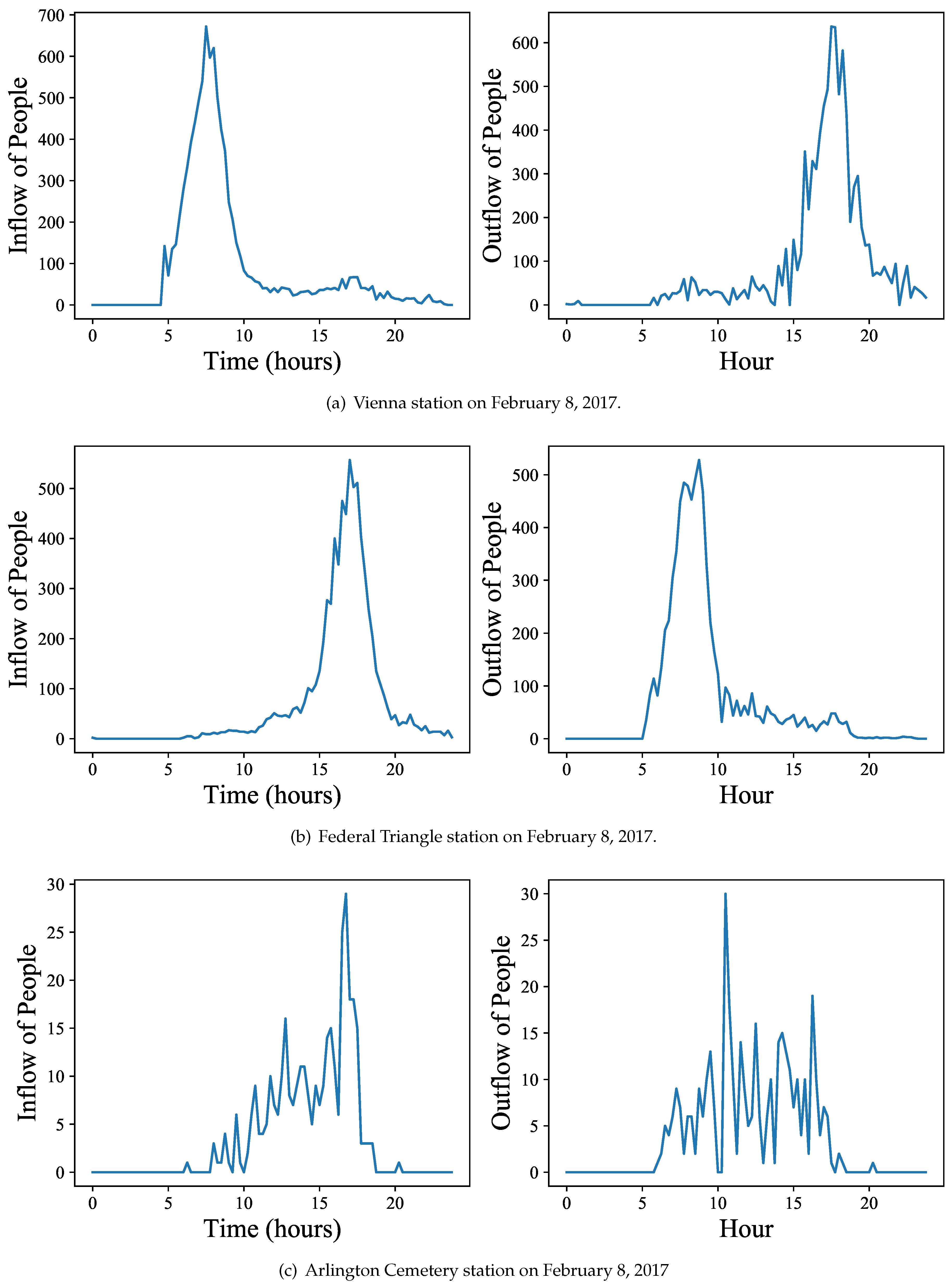
Figure 3.
Explained variance per principal component of the PCA on (a) the time series of stations and (b) the time series of days.
Figure 3.
Explained variance per principal component of the PCA on (a) the time series of stations and (b) the time series of days.

Figure 4.
Clustering of the stations for all the days: part of the dendrogram.

Figure 5.
Elbow curve for the selection of the number of station clusters.

Figure 6.
Spatial distribution of 5-Means clustering of latent features of the stations.

Figure 7.
Elbow curve for the selection of the number of clusters of days.

Figure 8.
K-Means clustering of the days over all the stations.

Figure 9.
kNN Classification accuracy of metro station labels: effect of k.
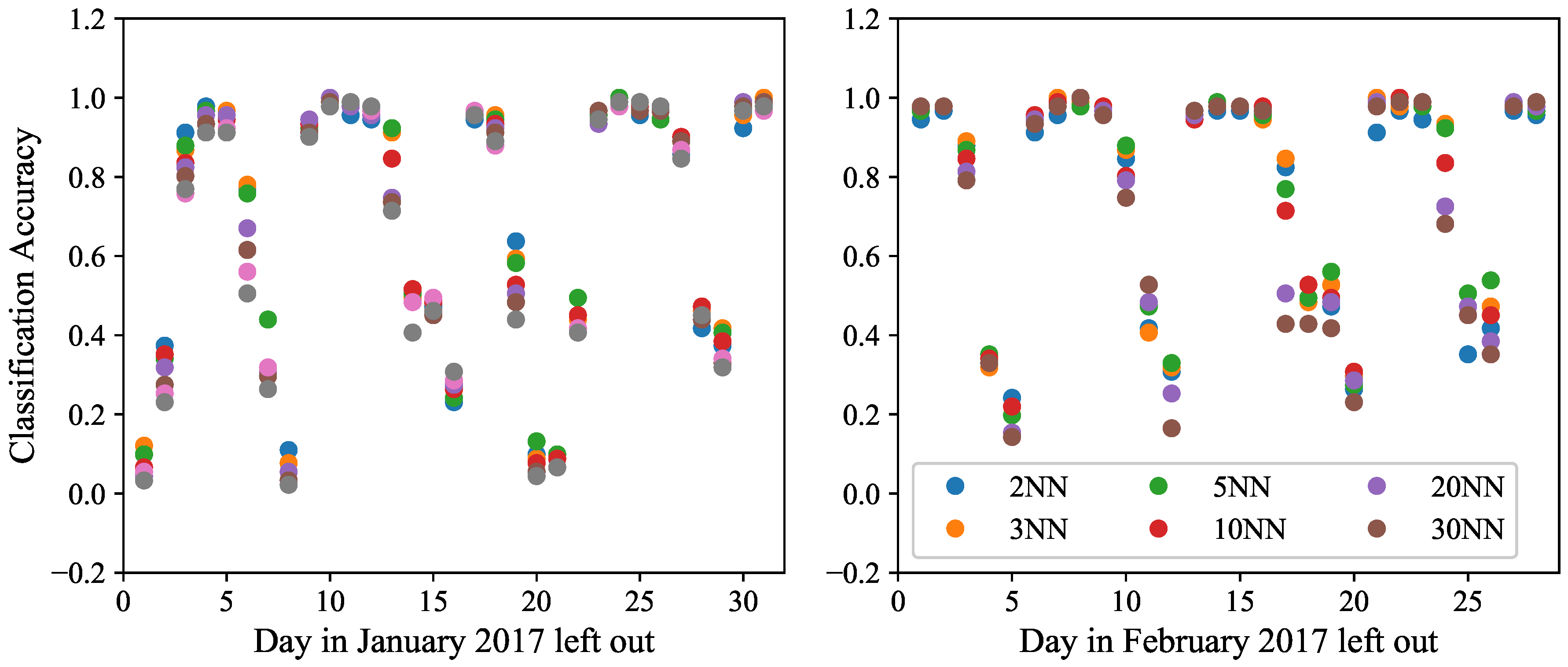
Figure 10.
Classification accuracy of metro station labels and cluster labels.
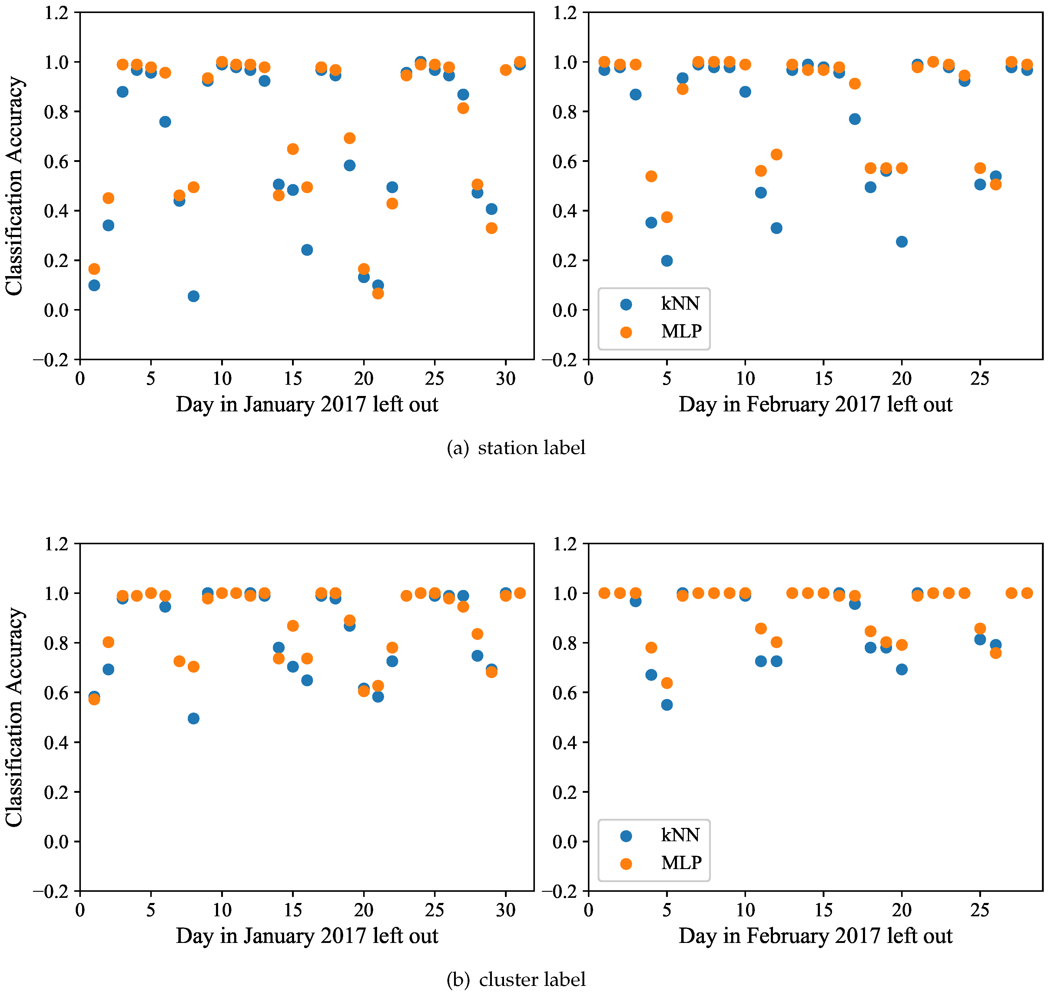
Figure 11.
Absolute prediction error: kNN vs. MLP artificial neural networks of varying settings.

Figure 12.
Absolute prediction error: kNN vs. weekly and daily periodicity prediction.

Figure 13.
Absolute prediction error: kNN vs. weekly and daily periodicity prediction of the three station clusters.
Figure 13.
Absolute prediction error: kNN vs. weekly and daily periodicity prediction of the three station clusters.

Figure 14.
Relative reduction of the prediction error for the metro data.
© 2018 by the authors. Licensee MDPI, Basel, Switzerland. This article is an open access article distributed under the terms and conditions of the Creative Commons Attribution (CC BY) license (http://creativecommons.org/licenses/by/4.0/).
Share and Cite
MDPI and ACS Style
Truong, R.; Gkountouna, O.; Pfoser, D.; Züfle, A. Towards a Better Understanding of Public Transportation Traffic: A Case Study of the Washington, DC Metro. Urban Sci. 2018, 2, 65. https://doi.org/10.3390/urbansci2030065
AMA Style
Truong R, Gkountouna O, Pfoser D, Züfle A. Towards a Better Understanding of Public Transportation Traffic: A Case Study of the Washington, DC Metro. Urban Science. 2018; 2(3):65. https://doi.org/10.3390/urbansci2030065
Chicago/Turabian StyleTruong, Robert, Olga Gkountouna, Dieter Pfoser, and Andreas Züfle. 2018. "Towards a Better Understanding of Public Transportation Traffic: A Case Study of the Washington, DC Metro" Urban Science 2, no. 3: 65. https://doi.org/10.3390/urbansci2030065