Article

Development of a Semi-Empirical Model for Estimating the Efficiency of Thermodynamic Power Cycles

Department of Thermal Engineering, School of Mechanical Engineering, National Technical University of Athens, 15780 Athens, Greece
Submission received: 29 June 2023 / Revised: 17 August 2023 / Accepted: 22 August 2023 / Published: 24 August 2023

Abstract

:
Power plants constitute the main sources of electricity production, and the calculation of their efficiency is a critical factor that is needed in energy studies. The efficiency improvement of power plants through the optimization of the cycle is a critical means of reducing fuel consumption and leading to more sustainable designs. The goal of the present work is the development of semi-empirical models for estimating the thermodynamic efficiency of power cycles. The developed model uses only the lower and the high operating temperature levels, which makes it flexible and easily applicable. The final expression is found by using the literature data for different power cycles, named as: organic Rankine cycles, water-steam Rankine cycles, gas turbines, combined cycles and Stirling engines. According to the results, the real operation of the different cases was found to be a bit lower compared to the respective endoreversible cycle. Specifically, the present global model indicates that the thermodynamic efficiency is a function of the temperature ratio (low cycle temperature to high cycle temperature). The suggested equation can be exploited as a quick and accurate tool for calculating the thermodynamic efficiency of power plants by using the operating temperature levels. Moreover, separate equations are provided for all of the examined thermodynamic cycles.

1. Introduction

1.1. Power Plants Efficiency

The global energy demand will increase by 50% between 2020 and 2050 [1], which will also lead to a 25% increase in CO2 emissions on a yearly basis [2]. The population increase and new lifestyle trends are basic reasons for the present and future energy situation. Power plants produce the majority of the required electricity; therefore, great interest is given to them, with the aim of increasing their performance [3]. Moreover, the incorporation of renewable energies (e.g., solar energy [4]) is vital for reducing the associated CO2 emissions. The optimization of power plants [5] is also an important weapon for achieving sustainability and leading to suitable units that are ideal for reducing the cost of electricity and simultaneously increasing CO2 avoidance. Another important option is the optimization of power cycles in order to increase their thermodynamic efficiency, which would reduce fuel consumption and consequently lead to sustainable designs.

1.2. Brief Literature Review

Quick and simplistic methods for the estimation of power plants’ efficiency are an issue that has been examined by various researchers. Theoretical thermodynamic studies have been performed to determine the optimal operating conditions of power plants. Usually, the operating temperature levels of the thermodynamic cycles are used in the examined models because they play a critical role in the efficiency. Specifically, the temperatures commonly incorporated in the calculations are related to the temperatures of the heat sinks that communicate with the power cycles (heat input and heat rejection sinks). Also, there are models that incorporate extra parameters like the capacity and the heat transfer coefficients.
The theoretical maximum limit for the thermodynamic efficiency of the power cycle is determined by the Carnot ideal cycle, using the low cycle temperature (Tlow) and the high cycle temperature (Thigh), as shown below [6]:
η c a r n o t = 1 T l o w T h i g h
However, the Carnot cycle is the theoretical ideal cycle and cannot be achieved in real life. Therefore, a more realistic approach has been suggested by Curzon and Ahlborn [7], which indicates lower thermodynamic efficiency values. Specifically, this formula takes the real heat transfer from the hot and cold sinks into consideration, but it assumes a Carnot cycle after the heat transfer. Thus, there is an endoreversible cycle, where the efficiency can be found below [7]:
η e n d o r = 1 T l o w T h i g h
Through the application of Taylor’s theory, the endoreversible efficiency can be written, as below, by giving the first three factors of the polynomial approximation expression [8]:
η e n d o r = 1 1 η c a r n o t η c a r n o t 2 + ( η c a r n o t ) 2 8 + 6 ( η c a r n o t ) 3 96 +
Interestingly, the previous formula indicates that the endoreversible efficiency is a bit higher than half of the Carnot efficiency—an interesting result that can be exploited for the cycle efficiency analysis.
Considering the maximum high temperature as the exergetically equivalent temperature, then the cycle efficiency can be written as below, according to Bejan [9]:
η t h = 1 T l o w T h i g h 1 + ln T h i g h T l o w
The previous formula also considers the power plant as an obstacle between the high and low heat sinks.
Assuming that a heat engine operates at ecological optimization conditions, the thermodynamic efficiency can be written as below [10,11]:
η t h = 1 T l o w T h i g h 1 + T h i g h T l o w 2
A generalized approach uses the irreversibility (i) and leads to the following cycle efficiency, which has been suggested by Novikov [6,12]:
η e n d o r = 1 1 + i T l o w T h i g h
Another general approach uses the superscript (a) in the temperature ratio, as below [13]. The following expression can approximate any cycle by selecting the suitable value of parameter (a):
η t h = 1 T l o w T h i g h a
The use of infinite reversible Carnot cycles together leads to the concept of the “poly-cycle”, which presents the following theoretical efficiency [14]:
η t h = 1 + 1 η c a r n o t η c a r n o t ln 1 η c a r n o t
The theoretical efficiency of a combined cycle, using endoreversible sub-cycles, is given by also introducing the medium heat exchange temperature (Tm) [15]:
η t h , c c = 1 T m T h i g h + 1 T l o w T m T m T h i g h
Therefore, it is clear that there is great interest in the literature for thermodynamic cycle performance with various suggested formulas. Different modeling and approximation strategies lead to different expressions. However, the common point of the summarized modeling is the use of the operating temperatures for the estimation of the thermodynamic efficiencies. This fact indicates that the temperatures are the critical parameters for the efficiency of power plants. Also, many equations correlate the thermodynamic efficiency of the cycle with the maximum lit of the Carnot cycle, which, in practice, means a direct connection with the operating temperature levels.

1.3. The Scope of the Present Work

The previous analysis proves that significant research has been conducted with the aim of estimating power plant efficiency. Numerous researchers have developed theoretical equations that can estimate the cycle efficiency in a realistic way, by applying different “boundary conditions” that simulate the real operation in a proper way. However, the majority of the literature studies are theoretical and do not use practical data (e.g., experimental or simulation results). In this direction, the present work aims to fill this scientific gap by developing a semi-empirical model that estimates power plant efficiency in a proper way using the literature data. This model uses the generalized formula of engine efficiency and also employs the literature data to properly fit the general model to the data. The analysis is performed for different power cycles, and a global model is suggested, which can be applied to every thermodynamic cycle. The final results of the present work can be exploited in the future for the accurate and quick estimation of the power plants’ efficiency—something that is important in optimization procedures, environmental studies, as well as in economic investigations. The use of the developed semi-empirical models can accelerate performance improvement and the design of future power plants for achieving sustainability.

2. Material and Methods

2.1. Basic Mathematical Background

The present work is based on the exploitation of the generalized expression for the thermodynamic efficiency (ηth) of a heat engine. More specifically, the following expression is used [13]:
η t h = 1 T l o w T h i g h a
where the low cycle temperature (Tlow) and the high cycle temperature (Thigh) are used in the previous formula, while parameter (a) determines the cycle’s performance. Specifically, the different values of the parameter (a) can lead to different cases of the usual thermodynamic cycles.
For a = 1, Equation (10) represents the Carnot cycle, as below [6]:
η t h a = 1 = η c a r n o t = 1 T l o w T h i g h
For a = 1/2, Equation (10) indicates the Curzon–Ahlborn equations, which correspond to an endoreversible cycle performance [7]:
η t h a = 1 2 = η e n d o r = 1 T l o w T h i g h
For the case with (a = 0), the cycle has zero efficiency and it cannot produce useful work. Therefore, the present expression can model every possible cycle that has a performance from zero up to the maximum Carnot cycle limit. In this direction, the maximum value for the parameter (a) is determined to be 1 (a ≤ 1) because higher values lead to non-acceptable thermodynamic efficiency values.
In cases where the cycle temperatures and efficiency are known, then superscript (a) can be calculated as below [16]:
a = ln 1 η t h ln T l o w T h i g h
An alternative expression of superscript (a), using the cycle efficiency (ηth) and the respective Carnot cycle efficiency (ηcarnot), is given below:
a = ln 1 η t h ln 1 η c a r n o t
The previous expressions can be used for the proper analysis of the data obtained from the literature studies for the calculation of parameter (a).

2.2. Followed Methodology

In the present work, the literature data have been used in order to summarize the thermodynamic efficiency of different power cycles. In each case, the low cycle temperature (Tlow), the high cycle temperature (Thigh) and the cycle efficiency (ηth) are extracted, aiming to estimate superscript (a), which describes the cycle behavior according to Equation (10). Linear regression methods are applied to estimate the suitable values of parameter (a) in every case. In this work, data for various cycles have been used, and more specifically, for the organic Rankine cycle (ORC), water-steam Rankine cycle (WS-RC), Stirling engine, combined cycle (CC), air gas turbine (Air-GT) and supercritical carbon dioxide gas turbine (SCO2-GT). The maximum examined temperature is 1800 K for the air gas turbine, while the minimum is 353 K for ORC. It is useful to state that the data for the ORC were separated into two categories: one for low-temperature ORC (LT-ORC) and one for high-temperature ORC (HT-ORC). The low-temperature ORC presents a maximum cycle temperature of up to 110 °C, while the cases with higher temperatures are included in the high-temperature ORC.
For each case, parameter (a) is calculated, as well as for every team of data that corresponds to a specific power cycle. Moreover, all the data will be examined together to determine the global value of the parameter (a) and the final results will be discussed. Finally, the reported data will be compared with the theoretical curves for the Carnot cycle and the endoreversible cycle.

3. Results and Discussion

The present section is devoted to including the results of the present analysis regarding the performance of the thermodynamic cycle and regression with the model presented in this paper. Table 1 summarizes the studies included in the present analysis, including the operating temperature levels, the reported thermodynamic efficiency, as well as the calculated efficiency of the respective Carnot cycle and endoreversible cycle. Specifically, there are data from 15 different works, as reported in Table 1. Forty-two different cases are included for seven different cycle types. Also, both experimental and theoretical data were used in the present analysis, as reported in Table 1. For every study, parameter (a) is determined for estimating the cycle efficiency (ηth) according to Equation (10), and the results are reported in Table 1. Moreover, the respective results for the Carnot and the nonreversible cycle are reported. It is clear that the Carnot efficiency is always greater than the reported efficiency, while the endoreversible efficiency is close to the reported efficiency data. Moreover, it is useful to add that the endoreversible efficiency is a bit higher than the respective Carnot efficiency, as was mentioned in the introduction part regarding Equation (3).
Figure 1 depicts the reported data by classifying them according to the power cycle type. Seven different categories were reported and the thermodynamic efficiency was given as a function of the high cycle temperature in Figure 1a and as a function of the temperature ratio (low temperature to high temperature) in Figure 1b. Table 2 summarizes the calculated superscripts (a) for the different cycles, and the regression coefficient (R2) is also given for every case. It is very important to highlight that parameter (a) was calculated with a linear regression of the logarithmic factors, according to Equation (10). It is obvious that the reported (R2) values are high; therefore, the regressions are assumed as reliable. Specifically, the values of (R2) ranged from 96.47% up to 99.91%—a fact that verifies the validity of the regression procedures.
More specifically, the following results are reported:
For the LT-ORC, the total (a) is found at 0.3481 while the reported results indicate a variation from 0.2996 up to 0.3753.
For the HT-ORC, the total (a) is found at 0.5813 while the reported results indicate a variation from 0.4770 up to 0.6399.
For the WS-RC, the total (a) is found at 0.5295 while the reported results indicate a variation from 0.4750 up to 0.5793.
For the Stirling cycle, the total (a) is found at 0.4267 while the reported results indicate a variation from 0.3432 up to 0.5653.
For the SCO2-GT, the total (a) is found at 0.5189 while the reported results indicate a variation from 0.5051 up to 0.5470.
For the Air-GT, the total (a) is found at 0.4808 while the reported results indicate a variation from 0.4617 up to 0.4929.
For the CC, the total (a) is found at 0.4220 while the reported results indicate a variation from 0.3667 up to 0.4440.
The increase in parameter (a) means a higher performance and this renders the cycle close to the respective ideal one (Carnot where a = 1). The highest values of the parameter (a) were found for the HT-ORC, WS-RC and SCO2-GT, while the next cycles that follow are the Air-GT, Stirling cycle, combined cycle and LT-ORC, respectively. At this point, it is critical to state that value (a) can be variable when a thermodynamic cycle is optimized, but the present results give a general overview of typical cycle cases.
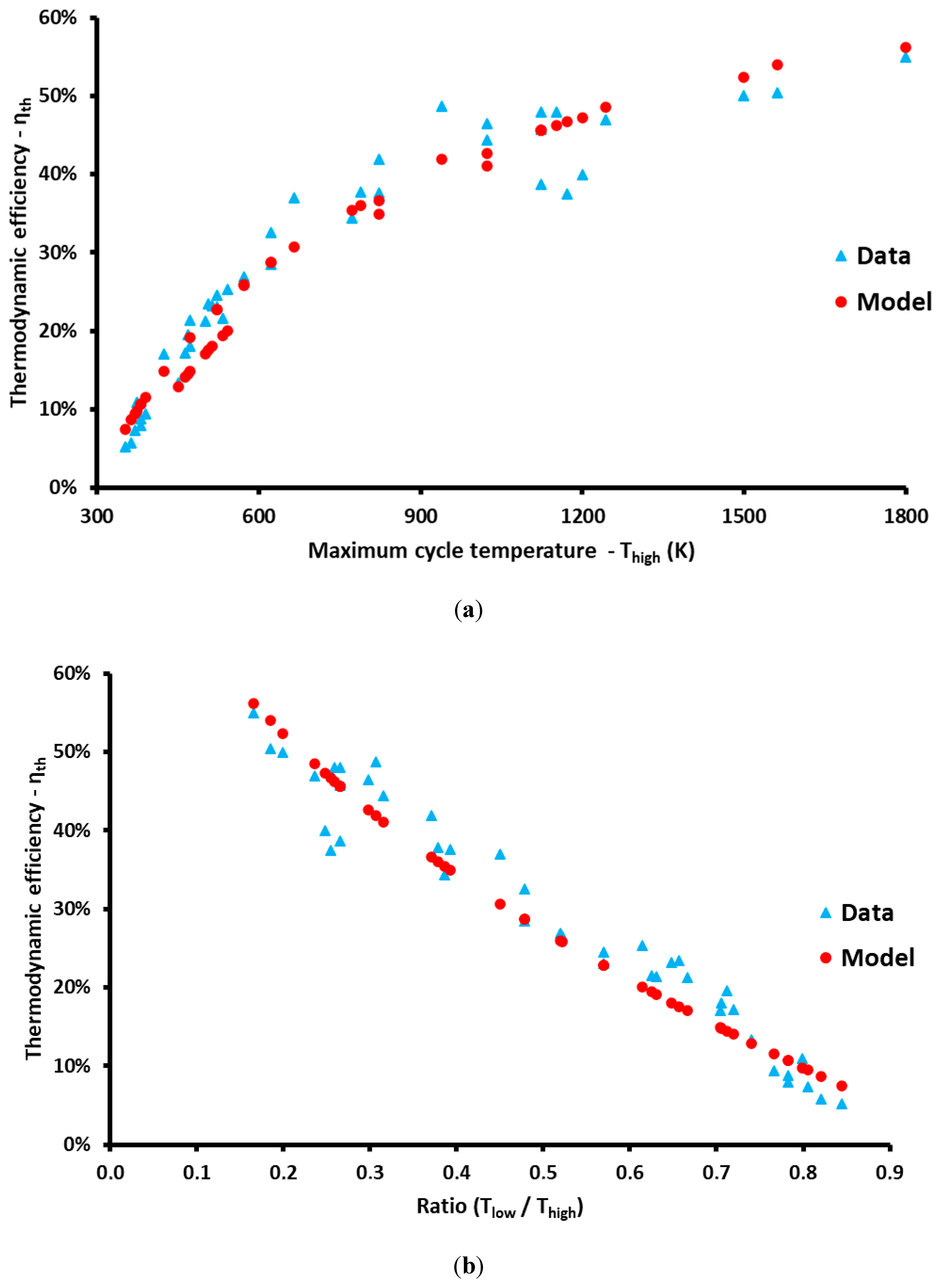
The total set of the 42 reported cases leads to the global value of the parameter (a) of 0.4594, as is given in Table 2. The (R2) is 98.06% for this case, and thus this regression is acceptable. Figure 2 depicts the reported data and the approximated data with the calculated approximation model. Specifically, Figure 2a shows the thermodynamic efficiency results for different values of the high cycle temperature, while in Figure 2b, they are shown as a function of the temperature ratio (low temperature to high temperature). The global approximation model for all the cycles is described by the next equation:
η t h , a p p r = 1 T l o w T h i g h 0.4594
It is obvious that the real collected data are very close to the data that are produced by the aforementioned approximation model. Thus, there is also a graphical verification of the developed model and it is clear that the developed model gives reasonable results. This note makes it clear that the created model can be used for future calculations of power cycle efficiencies. It constitutes a quick and accurate tool for estimating the efficiency of the power cycle by knowing two critical parameters: the low and the high cycle temperature levels. Moreover, this formula can be used for optimization studies of power cycles (e.g., coupling with solar thermal system).
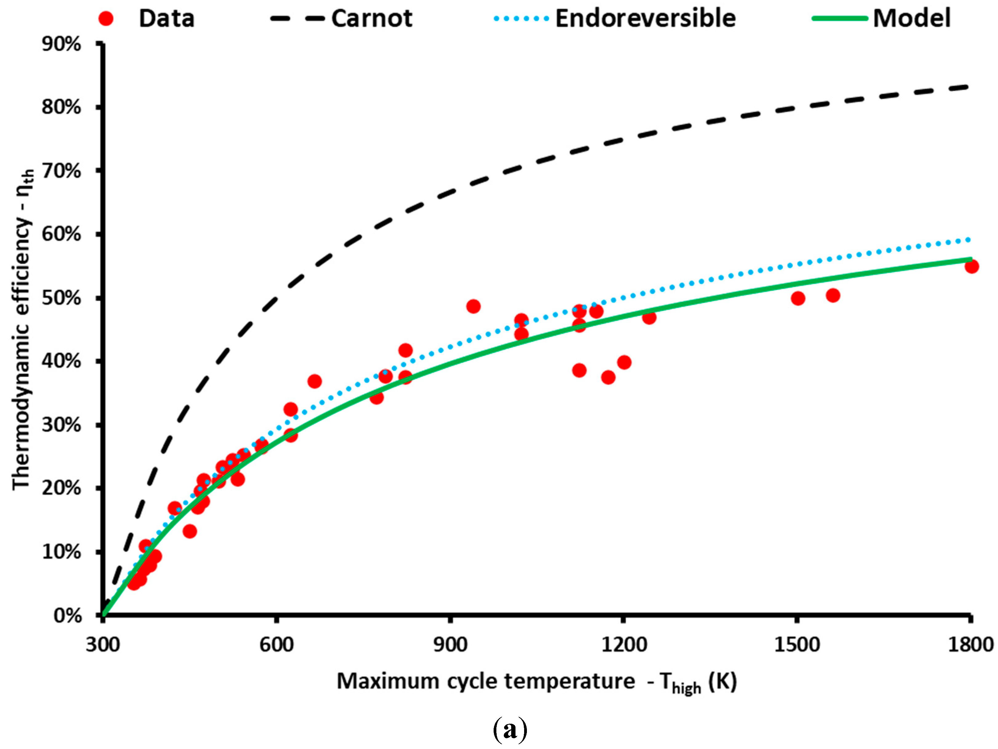
In the last part of the analysis, Figure 3 depicts the correlation of the reported data and of the developed expression with the curves of the Carnot efficiency and the endoreversible efficiency. Specifically, Figure 3a shows the results for different values of the high cycle temperature, while in Figure 3b, they are shown as a function of the temperature ratio (low temperature to high temperature). It is clear that the Carnot efficiency curves have a significant deviation from the reported results; however, this is reasonable and acceptable. On the other hand, the developed Equation (15) is close to the endoreversible efficiency curve, which indicates that the real operation is close to the endoreversible or the Curzon–Ahlborn cycle. However, the real operation is found to be a bit lower, as is obvious in Figure 3. The reported deviations of the data compared to the curves are explained by the existence of extra variables that influence the results, such as the isentropic efficiency, the working fluid selection, the use of regenerators, etc.
The greatest deviations were reported for high temperatures around 1200 K; however, in these cases, the deviation is also acceptable. On the other hand, the calculation with the suggested model is closer to the data in the low- and high-cycle temperature cases. Additionally, the results of Figure 1 and Figure 2 indicate that all the cycles generally obey the suggested rule, with the results for the Stirling Engine presenting some greater deviations. In this case, the R2 is found to be 96.47%, which is the smallest reported value among the cycles; however, it is an acceptable value for the present analysis.
In the future, the developed formula (Equation (15)) can be used as an acceptable and reliable tool for estimating power plant efficiency using only the basic operating temperature levels. Also, the present model can be used for optimization studies, for example, for increasing the cycle performance, for investigating solar-driven cycles, etc.

4. Conclusions

The objective of this investigation is the development of semi-empirical models for estimating the thermodynamic efficiency of power cycles. The developed models only use the lower and higher operating temperature levels. The final expression is found by using the literature data for different power cycles: organic Rankine cycles, water-steam Rankine cycles, gas turbines, combined cycles and Stirling engines. This model can be used for the estimation of the thermodynamic efficiency of power cycles, for the optimization of the cycles, as well as for investigating the coupling of the thermodynamic cycles with renewable energy sources (e.g., solar thermal collectors).
According to the results, the real operation of the different cases was found to be a bit lower compared to the respective endoreversible cycle. Specifically, the present global model indicates that the thermodynamic efficiency is a function of the temperature ratio, as below:
T h e r m o d y n a m i c   e f f i c i e n c y = 1 L o w   c y c l e   t e m e p r a t u r e H i g h   c y c l e   t e m e p r a t u r e 0.4594
The aforementioned formula can be used as a quick and accurate tool for estimating the thermodynamic efficiency of power plants by using the minimum possible input data. It presents an R2 of 98.06%, which indicates high accuracy. Also, different equations have been separately developed for each power cycle with high-accuracy indexes. More specifically, the following points describe the examined cycles:
In the LT-ORC case, the mean (a) is found at 0.3481 while the reported results indicate a variation from 0.2996 up to 0.3753.
In the HT-ORC case, the mean (a) is found at 0.5813 while the reported results indicate a variation from 0.4770 up to 0.6399.
In the WS-RC case, the mean (a) is found at 0.5295 while the reported results indicate a variation from 0.4750 up to 0.5793.
In the Stirling cycle case, the mean (a) is found at 0.4267 while the reported results indicate a variation from 0.3432 up to 0.5653.
In the SCO2-GT case, the mean (a) is found at 0.5189 while the reported results indicate a variation from 0.5051 up to 0.5470.
In the Air-GT case, the mean (a) is found at 0.4808 while the reported results indicate a variation from 0.4617 up to 0.4929.
In the CC case, the mean (a) is found at 0.4220 while the reported results indicate a variation from 0.3667 up to 0.4440.
In the future, it will be interesting to separately investigate how parameter (a) varies among the different topologies of each thermodynamic cycle by investigating a greater amount of data from the literature. Specifically, the impact of internal recuperators, heat exchangers, etc., on the parameter (a) can be examined, as well as the impact of different working fluids on the parameter (a). Moreover, a more complex model can be examined with two “free parameters” for estimating the cycles’ performance with greater accuracy. Specifically, parameter (a) can be modeled as a polynomial of other parameters in order to take extra design aspects of each cycle into consideration.

Funding

This research received no external funding.

Institutional Review Board Statement

Not applicable.

Informed Consent Statement

Not applicable.

Data Availability Statement

Data available after request.

Conflicts of Interest

The author declares no conflict of interest.

Nomenclature

aSuperscript of the temperature ratio
iIrreversibility factor
R2Regression coefficient
ThighHigh cycle temperature, K
TlowLow cycle temperature, K
TmMedium temperature, K
Greek Symbols
ηcarnotCarnot efficiency
ηendorEndoreversible efficiency
ηthThermodynamic efficiency
ηth,apprApproximated thermodynamic efficiency
Subscripts
maxMaximum reported value for the specific cycle type
minMinimum reported value for the specific cycle type
totalTotal value for the specific cycle type
Abbreviations
Air-GTAir Gas Turbine
CCCombined Cycle
EXPERExperimental work
HT-ORCHigh-Temperature Organic Rankine Cycle
LT-ORCLow-Temperature Organic Rankine Cycle
ORCOrganic Rankine cycle
SCO2-GTSupercritical Carbon Dioxide Gas Turbine
THEORTheoretical work
WS-RCWater-Steam Rankine Cycle

References

  1. World Energy Outlook—Topics. IEA n.d. Available online: https://www.iea.org/topics/world-energy-outlook (accessed on 26 June 2023).
  2. Ahmadi, M.H.; Ahmadi, M.A.; Sadatsakkak, S.A. Thermodynamic analysis and performance optimization of irreversible Carnot refrigerator by using multi-objective evolutionary algorithms (MOEAs). Renew. Sustain. Energy Rev. 2015, 51, 1055–1070. [Google Scholar] [CrossRef]
  3. Topel, M.; Laumert, B. Improving concentrating solar power plant performance by increasing steam turbine flexibility at start-up. Sol. Energy 2018, 165, 10–18. [Google Scholar] [CrossRef]
  4. Bellos, E. Progress in beam-down solar concentrating systems. Prog. Energy Combust. Sci. 2023, 97, 101085. [Google Scholar] [CrossRef]
  5. Porto-Hernandez, L.A.; Vargas, J.V.C.; Munoz, M.N.; Galeano-Cabral, J.; Ordonez, J.C.; Balmant, W.; Mariano, A.B. Fundamental optimization of steam Rankine cycle power plants. Energy Convers. Manag. 2023, 289, 117148. [Google Scholar] [CrossRef]
  6. Durmayaz, A.; Sogut, O.S.; Sahin, B.; Yavuz, H. Optimization of thermal systems based on finite-time thermodynamics and thermoeconomics. Prog. Energy Combust. Sci. 2004, 30, 175–217. [Google Scholar] [CrossRef]
  7. Curzon, F.L.; Ahlborn, B. Efficiency of a Carnot engine at maximum power output. Am. J. Phys. 1975, 43, 22–24. [Google Scholar] [CrossRef]
  8. Hernández, A.; Roco, J.M.; Medina, A.; Sánchez-Salas, N. Heat engines and the Curzon-Ahlborn efficiency. Rev. Mex. Fis. 2014, 60, 384. [Google Scholar]
  9. Bejan, A. Entropy generation minimization: The new thermodynamics of finite-size devices and finite-time processes. J. Appl. Phys. 1996, 79, 1191–1218. [Google Scholar] [CrossRef]
  10. Angulo-Brown, F. An ecological optimization criterion for finite-time heat engines. J. Appl. Phys. 1991, 69, 7465–7469. [Google Scholar] [CrossRef]
  11. Yan, Z. Comment on “An ecological optimization criterion for finite-time heat engines” [J. Appl. Phys. 69, 7465 (1991)]. J. Appl. Phys. 1993, 73, 3583. [Google Scholar] [CrossRef]
  12. Novikov, I.I. The efficiency of atomic power stations (a review). J. Nucl. Energy 1954 1958, 7, 125–128. [Google Scholar] [CrossRef]
  13. Badescu, V. Simple Upper Bound Efficiencies for Endoreversible Conversion of Thermal Radiation. J. Non-Equilib. Thermodyn. 1999, 24, 196–202. [Google Scholar] [CrossRef]
  14. Leff, H.S. Thermal Efficiency at Maximum Work Output: New Results for Old Heat Engines. Am. J. Phys. 1987, 55, 602–610. Available online: https://pubs.aip.org/aapt/ajp/article-abstract/55/7/602/1052998/Thermal-efficiency-at-maximum-work-output-New?redirectedFrom=fulltext (accessed on 27 June 2023). [CrossRef]
  15. Pinho, C. The Curzon-Ahlborn Efficiency of Combined Cycles; Academia: San Francisco, CA, USA, 2003. [Google Scholar]
  16. Chen, W.Z.; Sun, F.R.; Cheng, S.M.; Chen, L.G. Study on optimal performance and working temperatures of endoreversible forward and reverse carnot cycles. Int. J. Energy Res. 1995, 19, 751–759. [Google Scholar] [CrossRef]
  17. Iglesias Garcia, S.; Ferreiro Garcia, R.; Carbia Carril, J.; Iglesias Garcia, D. A review of thermodynamic cycles used in low temperature recovery systems over the last two years. Renew. Sustain. Energy Rev. 2018, 81, 760–767. [Google Scholar] [CrossRef]
  18. Rahbar, K.; Mahmoud, S.; Al-Dadah, R.K.; Moazami, N.; Mirhadizadeh, S.A. Review of organic Rankine cycle for small-scale applications. Energy Convers. Manag. 2017, 134, 135–155. [Google Scholar] [CrossRef]
  19. Tzivanidis, C.; Bellos, E.; Antonopoulos, K.A. Energetic and financial investigation of a stand-alone solar-thermal Organic Rankine Cycle power plant. Energy Convers. Manag. 2016, 126, 421–433. [Google Scholar] [CrossRef]
  20. Karellas, S.; Leontaritis, A.-D.; Panousis, G.; Bellos, E.; Kakaras, E. Energetic and exergetic analysis of waste heat recovery systems in the cement industry. Energy 2013, 58, 147–156. [Google Scholar] [CrossRef]
  21. Li, J.; Li, P.; Pei, G.; Alvi, J.Z.; Ji, J. Analysis of a novel solar electricity generation system using cascade Rankine cycle and steam screw expander. Appl. Energy 2016, 165, 627–638. [Google Scholar] [CrossRef]
  22. Pramanik, S.; Ravikrishna, R.V. A review of concentrated solar power hybrid technologies. Appl. Therm. Eng. 2017, 127, 602–637. [Google Scholar] [CrossRef]
  23. Carrillo Caballero, G.E.; Mendoza, L.S.; Martinez, A.M.; Silva, E.E.; Melian, V.R.; Venturini, O.J.; del Olmo, O.A. Optimization of a Dish Stirling system working with DIR-type receiver using multi-objective techniques. Appl. Energy 2017, 204, 271–286. [Google Scholar] [CrossRef]
  24. Ranieri, S.; Prado, G.A.O.; MacDonald, B.D. Efficiency Reduction in Stirling Engines Resulting from Sinusoidal Motion. Energies 2018, 11, 2887. [Google Scholar] [CrossRef]
  25. Toghyani, S.; Kasaeian, A.; Ahmadi, M.H. Multi-objective optimization of Stirling engine using non-ideal adiabatic method. Energy Convers. Manag. 2014, 80, 54–62. [Google Scholar] [CrossRef]
  26. Smith, L.; Nuel, B.; Weaver, S.P.; Berkower, S.; Gross, B. 25 kW Low-Temperature Stirling Engine for Heat Recovery, Solar, and Biomass Applications. In Proceedings of the 17th International Stirling Engine Conference (ISEC), Newcastle upon Tyne, UK, 24–26 August 2016. [Google Scholar]
  27. Sarkar, J.; Bhattacharyya, S. Optimization of recompression S-CO2 power cycle with reheating. Energy Convers. Manag. 2009, 50, 1939–1945. [Google Scholar] [CrossRef]
  28. Olumayegun, O.; Wang, M.; Kelsall, G. Closed-cycle gas turbine for power generation: A state-of-the-art review. Fuel 2016, 180, 694–717. [Google Scholar] [CrossRef]
  29. Ibrahim, T.K.; Mohammed, M.K.; Awad, O.I.; Rahman, M.M.; Najafi, G.; Basrawi, F.; Abd Alla, A.N.; Mamat, R. The optimum performance of the combined cycle power plant: A comprehensive review. Renew. Sustain. Energy Rev. 2017, 79, 459–474. [Google Scholar] [CrossRef]
  30. Ameri, M.; Ahmadi, P.; Khanmohammadi, S. Exergy analysis of a 420 MW combined cycle power plant. Int. J. Energy Res. 2008, 32, 175–183. [Google Scholar] [CrossRef]
  31. Polyzakis, A.L.; Koroneos, C.; Xydis, G. Optimum gas turbine cycle for combined cycle power plant. Energy Convers. Manag. 2008, 49, 551–563. [Google Scholar] [CrossRef]
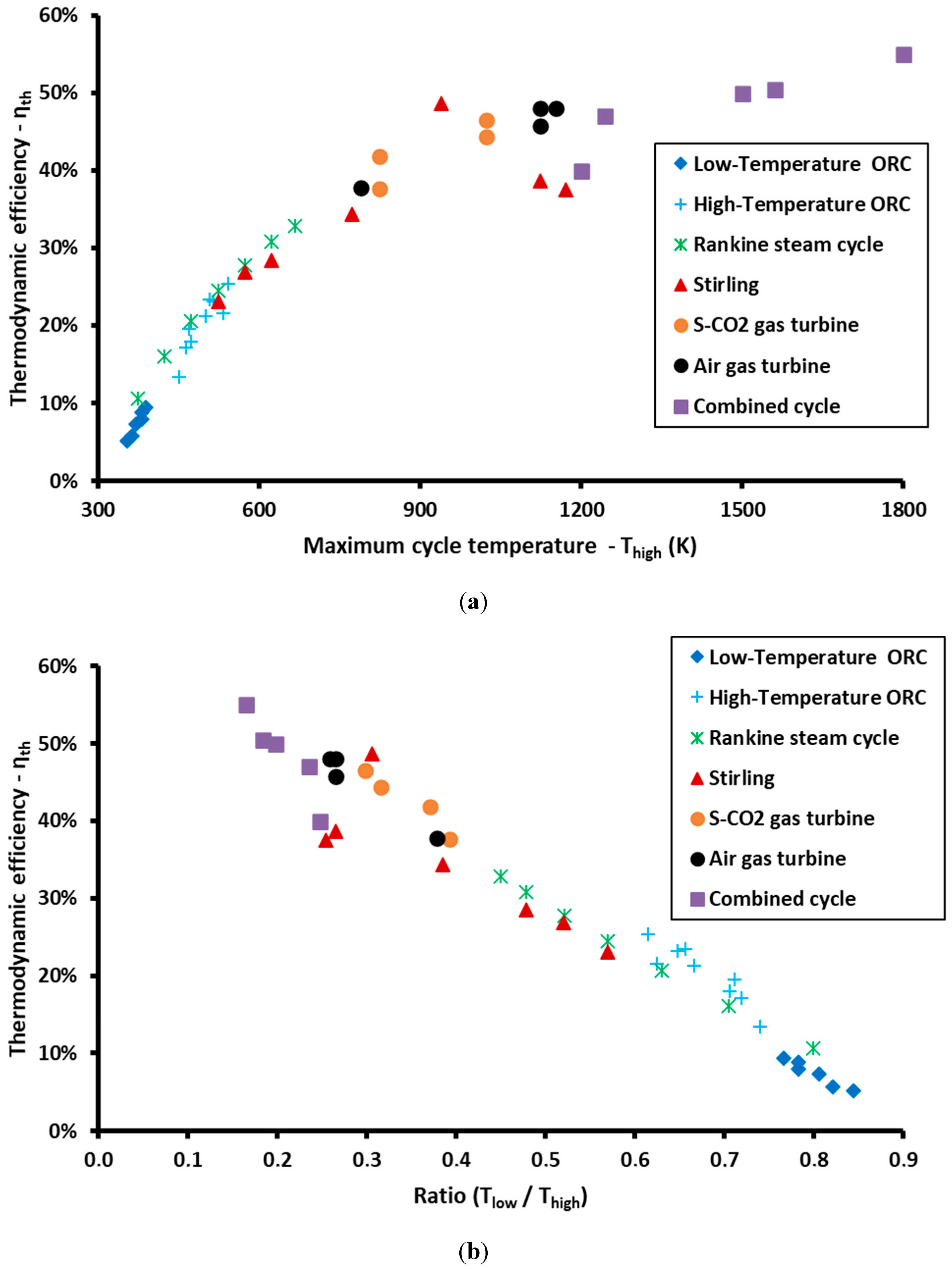
Figure 1. Thermodynamic cycle efficiency for different cycles (a) as a function of the high cycle temperature (Thigh); (b) as a function of the temperature ratio (Tlow/Thigh).
Sci 05 00033 g001
Figure 2. Thermodynamic cycle efficiency for all the reported data (a) as a function of the high cycle temperature (Thigh); (b) as a function of the temperature ratio (Tlow/Thigh).
Sci 05 00033 g002
Figure 3. Thermodynamic cycle efficiency for all the reported data, Carnot efficiency and endoreversible efficiency (a) as a function of the high cycle temperature (Thigh); (b) as a function of the temperature ratio (Tlow/Thigh).
Sci 05 00033 g003aSci 05 00033 g003b
Table 1. Literature input data in the present analysis.
N/AThigh (K)Tlow (K)ηthηcarnotηendoraCycleTypeRef.
13892980.09400.23390.12470.3704LT-ORCEXPER[17]
23812980.08810.21780.11560.3753LT-ORCEXPER[17]
33702980.07370.19460.10260.3538LT-ORCEXPER[17]
43632980.05740.17910.09390.2996LT-ORCTHEOR[17]
53532980.05220.15580.08120.3165LT-ORCEXPER[18]
63812980.07940.21780.11560.3367LT-ORCEXPER[18]
75423330.25360.38560.21620.6005HT-ORCTHEOR[19]
85073330.23410.34320.18960.6345HT-ORCTHEOR[19]
95143330.23160.35210.19510.6069HT-ORCTHEOR[19]
105333330.21550.37520.20960.5160HT-ORCTHEOR[19]
115003330.21250.33400.18390.5877HT-ORCTHEOR[19]
124683330.19570.28850.15650.6399HT-ORCTHEOR[19]
134723330.18000.29450.16010.5689HT-ORCTHEOR[19]
144633330.17140.28080.15190.5705HT-ORCTHEOR[19]
154503330.13380.26000.13980.4770HT-ORCTHEOR[19]
166232980.32600.52170.30840.5350WS-RCTHEOR[20]
173732980.10920.20110.10620.5151WS-RCTHEOR[21]
184232980.17020.29550.16070.5326WS-RCTHEOR[21]
194732980.21390.37000.20630.5209WS-RCTHEOR[21]
205232980.24510.43020.24520.4999WS-RCTHEOR[21]
215732990.26580.47820.27760.4750WS-RCTHEOR[21]
226663000.37000.54950.32880.5793WS-RCEXPER[22]
2311232980.38700.73460.48490.3689Stirling cycleEXPER[23]
2411722980.37500.74570.49580.3432Stirling cycleEXPER[23]
257732980.34400.61450.37910.4423Stirling cycleTHEOR[24]
269392880.48730.69330.44620.5653Stirling cycleTHEOR[25]
276232980.28500.52170.30840.4549Stirling cycleTHEOR[26]
285732980.26900.47990.27880.4793Stirling cycleTHEOR[26]
295232980.23100.43020.24520.4670Stirling cycleTHEOR[26]
308233050.41900.62940.39120.5470SCO2-GTTHEOR[27]
3110233050.46520.70190.45400.5172SCO2-GTTHEOR[27]
328233230.37650.60750.37350.5051SCO2-GTTHEOR[27]
3310233230.44400.68430.43810.5092SCO2-GTTHEOR[27]
3411232980.48000.73460.48490.4929Air-GTEXPER[28]
3511232980.45800.73460.48490.4617Air-GTEXPER[28]
3611522980.48000.74130.49140.4836Air-GTEXPER[28]
377882980.37800.62180.38500.4883Air-GTEXPER[28]
3812002980.40000.75170.50170.3667CCTHEOR[29]
3915002980.50000.80130.55430.4289CCTHEOR[29]
4018002980.55000.83440.59310.4440CCTHEOR[29]
4112442930.47000.76450.51470.4391CCEXPER[30]
4215612880.50470.81550.57050.4157CCTHEOR[31]
Table 2. Summary of the parameter (a) for the different cycles by using the logarithmic approximation of the reported results.
CycleatotalR2aminamax
Low-Temperature ORC0.348199.44%0.29960.3753
High-Temperature ORC0.581399.37%0.47700.6399
Water-Steam Rankine cycle0.529599.51%0.47500.5793
Stirling cycle0.426796.47%0.34320.5653
S-CO2 gas turbine0.518999.91%0.50510.5470
Air gas turbine0.480899.93%0.46170.4929
Combined cycle0.422099.63%0.36670.4440
TOTAL0.459498.06%--
Disclaimer/Publisher’s Note: The statements, opinions and data contained in all publications are solely those of the individual author(s) and contributor(s) and not of MDPI and/or the editor(s). MDPI and/or the editor(s) disclaim responsibility for any injury to people or property resulting from any ideas, methods, instructions or products referred to in the content.