Prediction of Vehicle Crashworthiness Parameters Using Piecewise Lumped Parameters and Finite Element Models

 ,
,
Abstract
:
1. Introduction
2. Materials and Methods
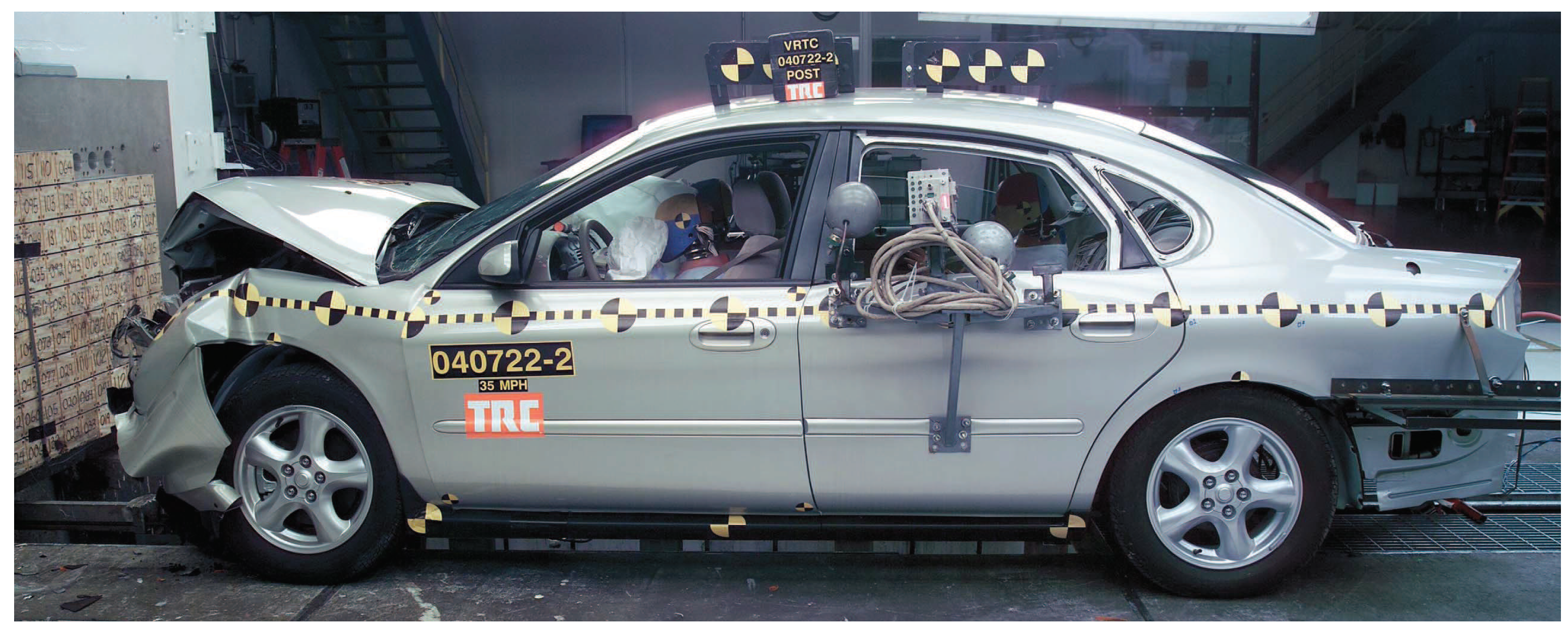
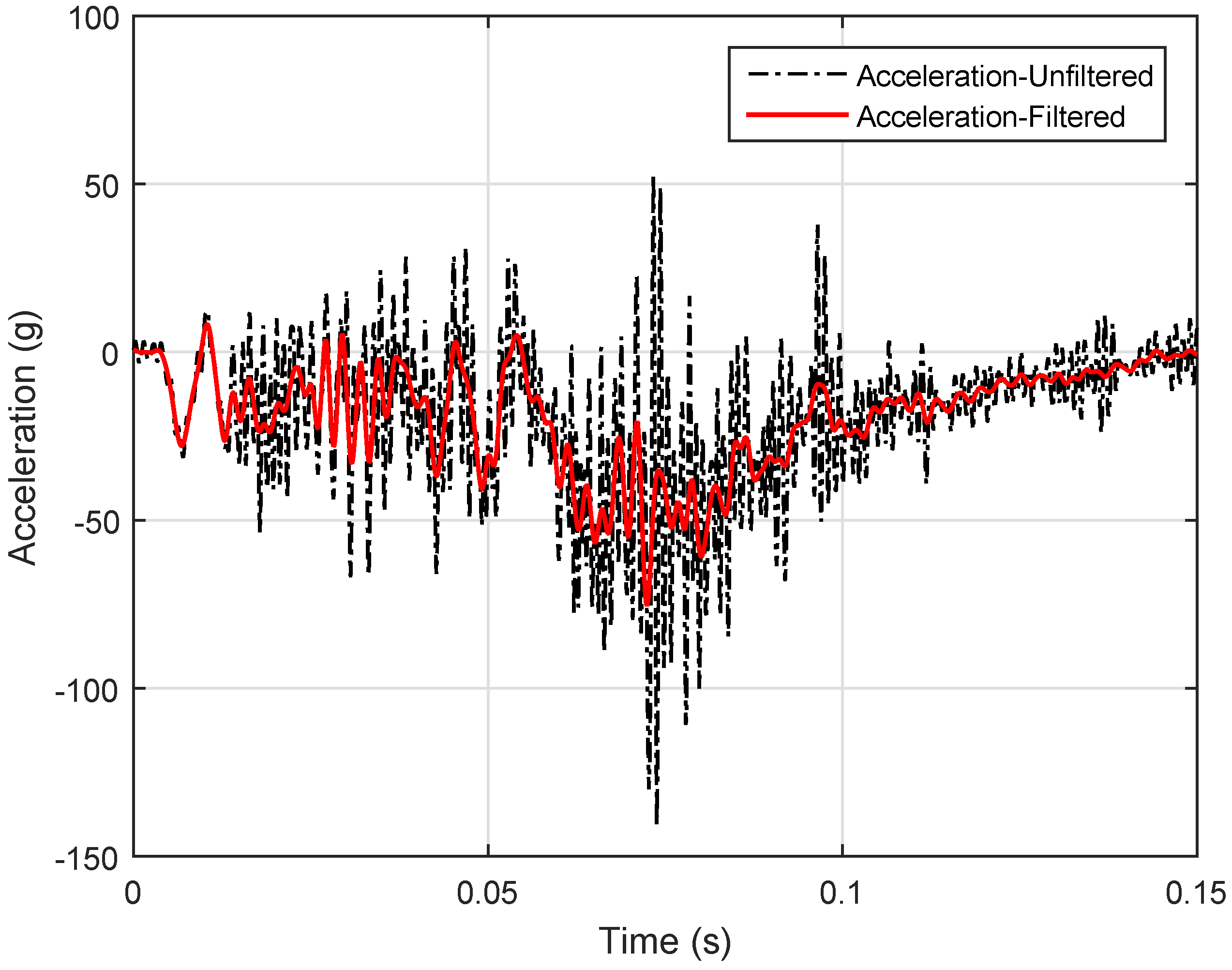
2.1. Experimental Data and Signal Filtering
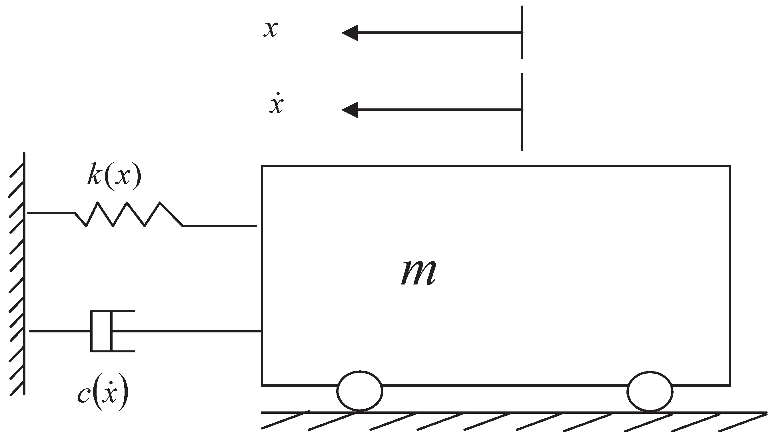
2.2. Piecewise Linear Lumped Parameters Model
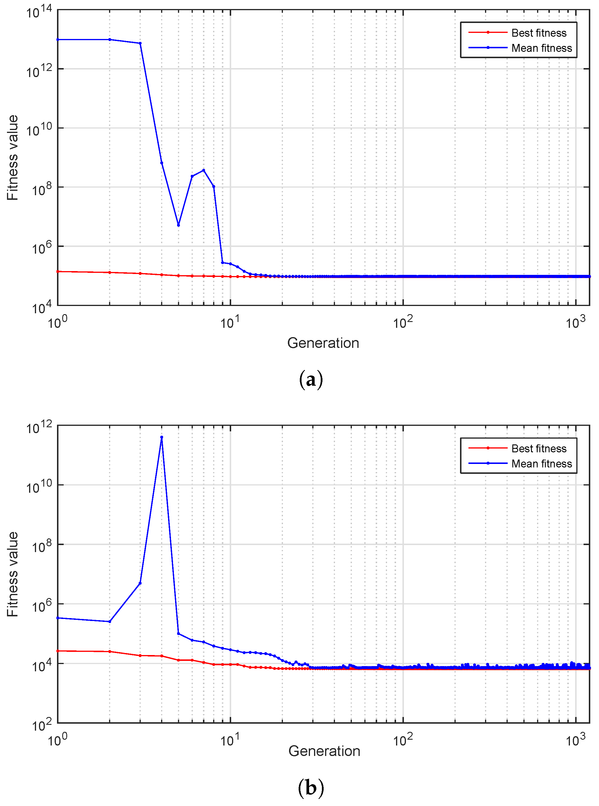
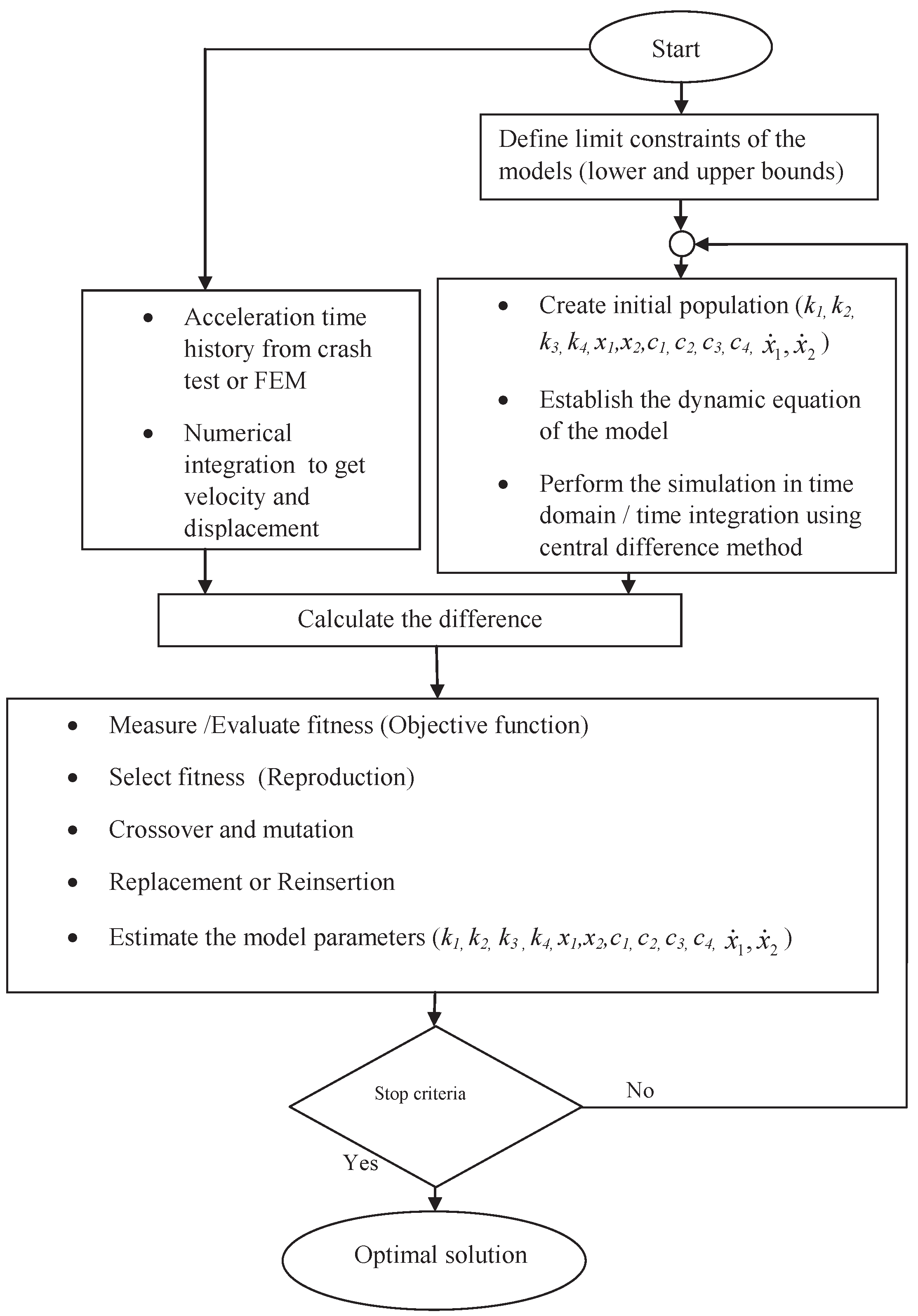
2.3. LPM Estimation and Calibration Scheme Using the Genetic Algorithm
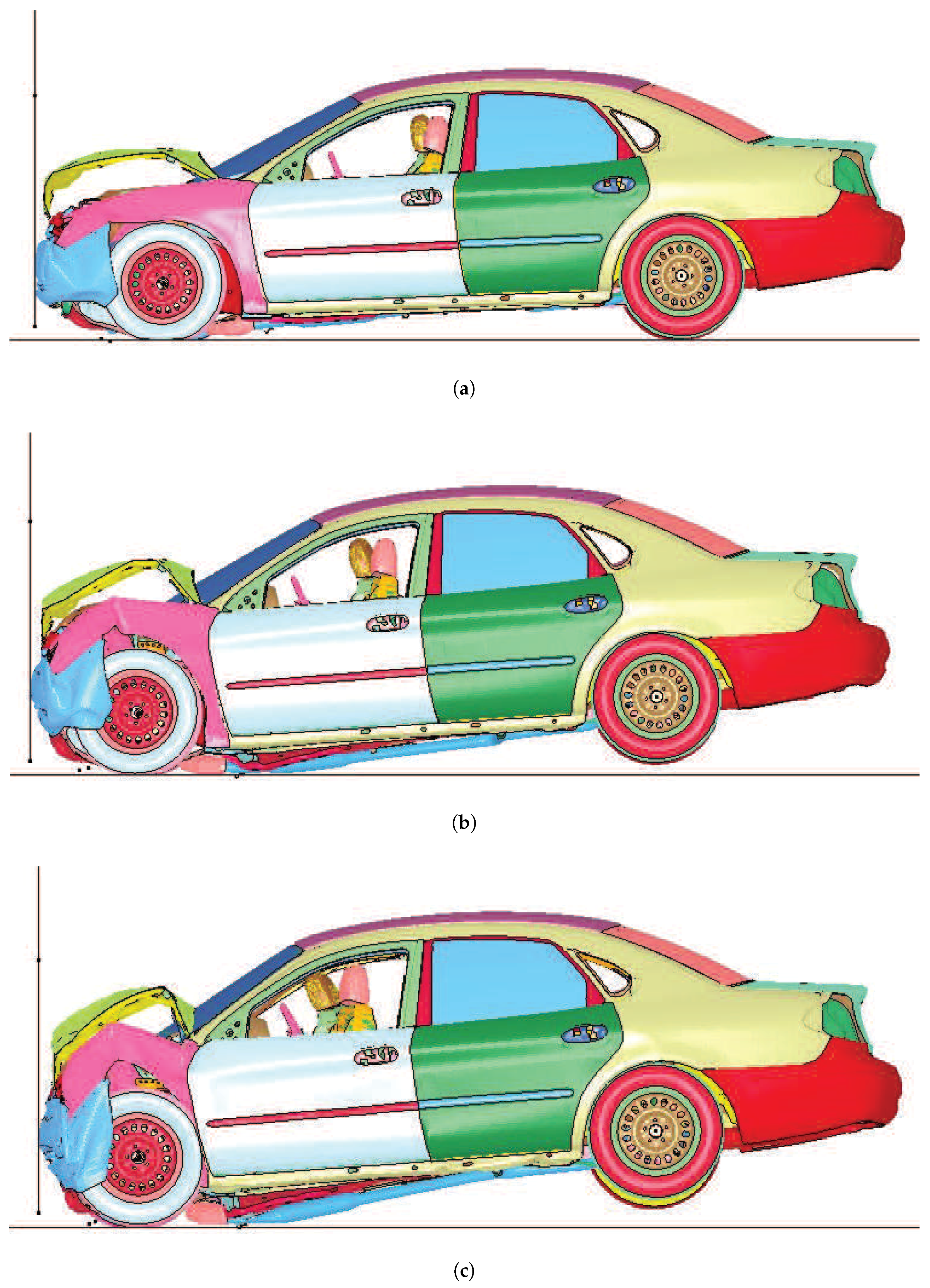
2.4. Finite Element Analysis
- Number of parts: 804,
- Number of nodes: 922,007,
- Number of beam elements: 10,
- Number of shell elements: 838,926,
- Number of solid elements: 134,468.
2.5. Acceleration Severity Index (ASI)
- Class A: ASI
- Class B: 1.0 ≤ ASI
- Class C: 1.4 ≤ ASI
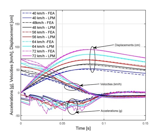
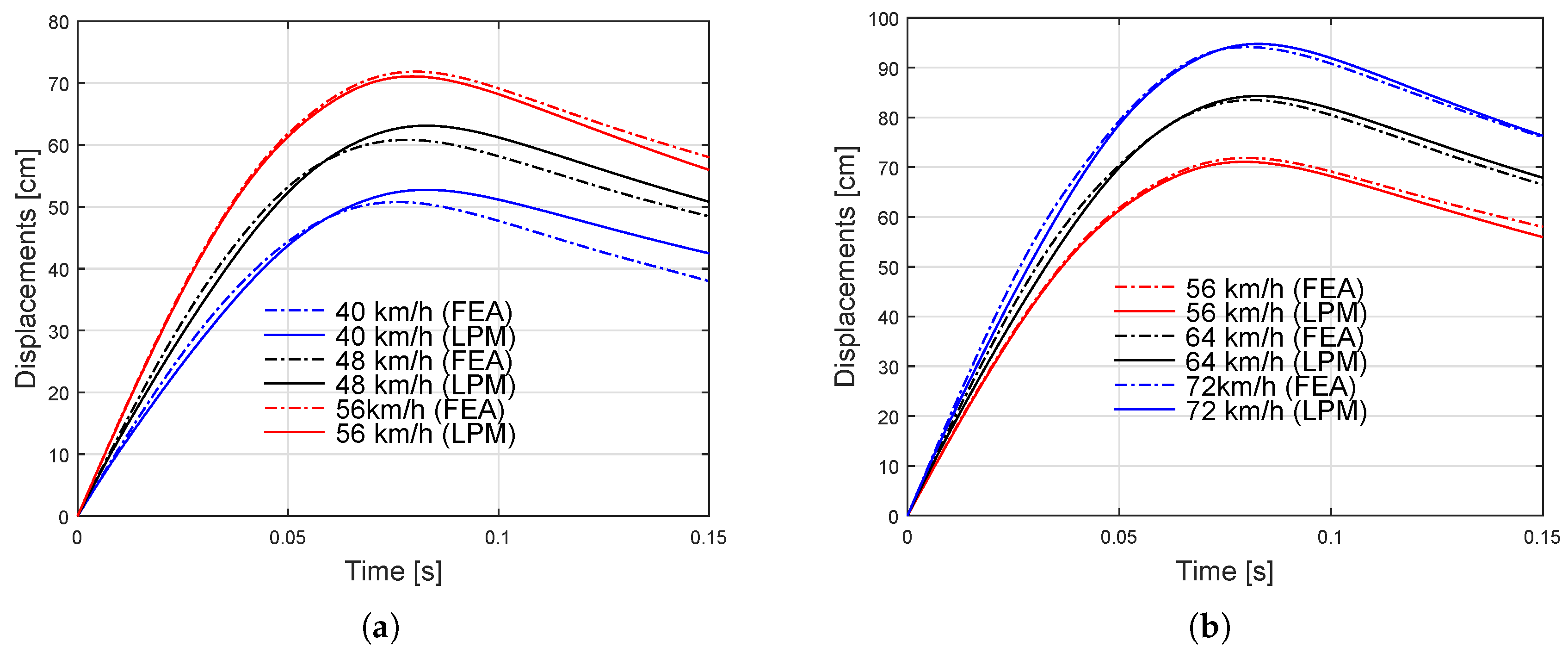
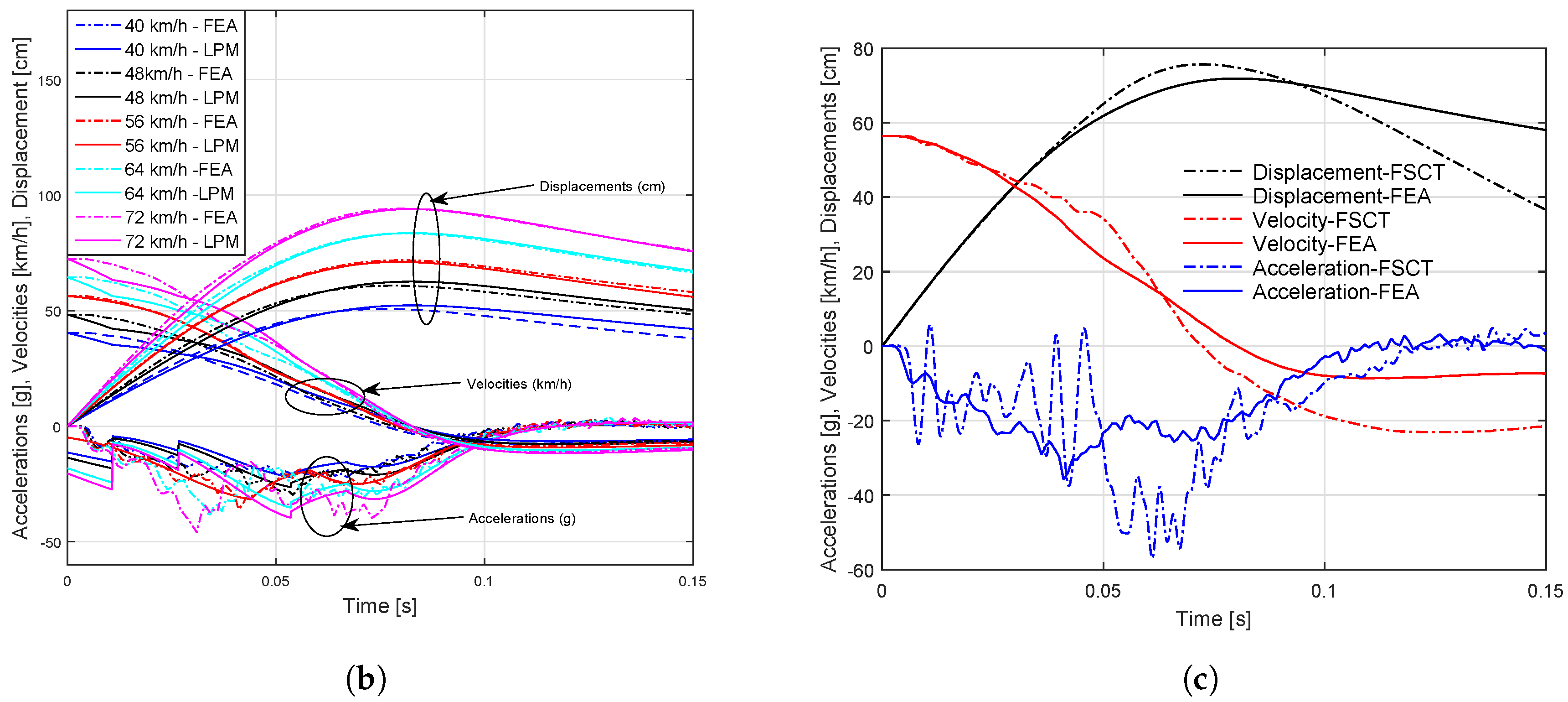
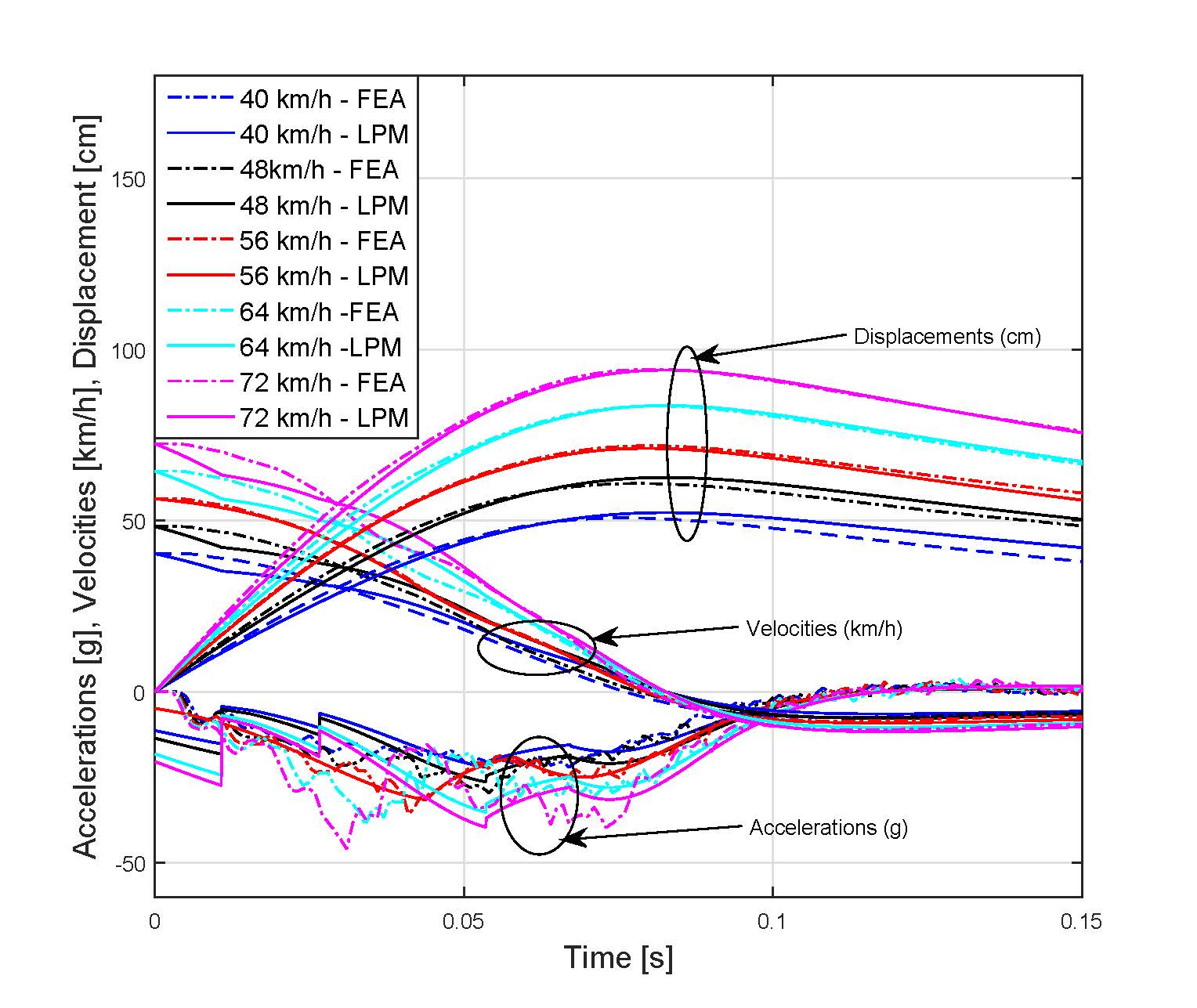
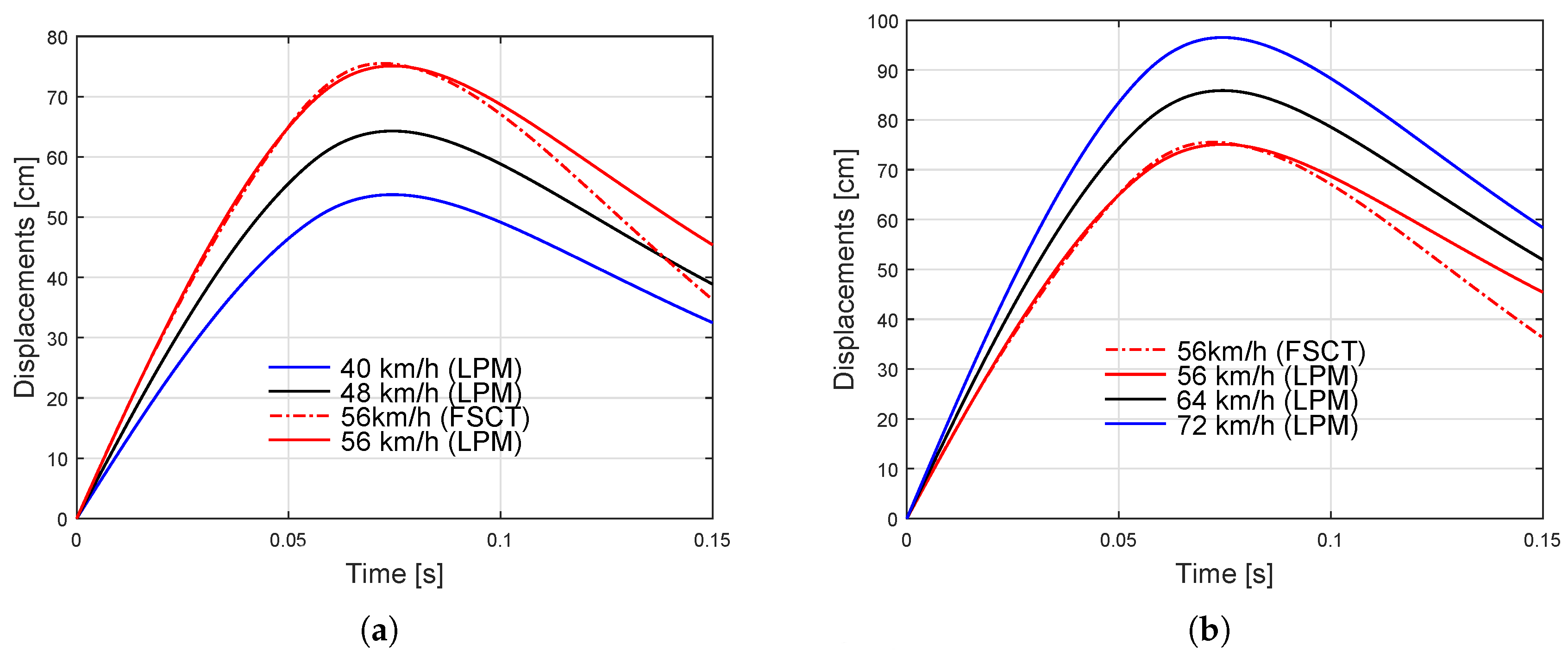
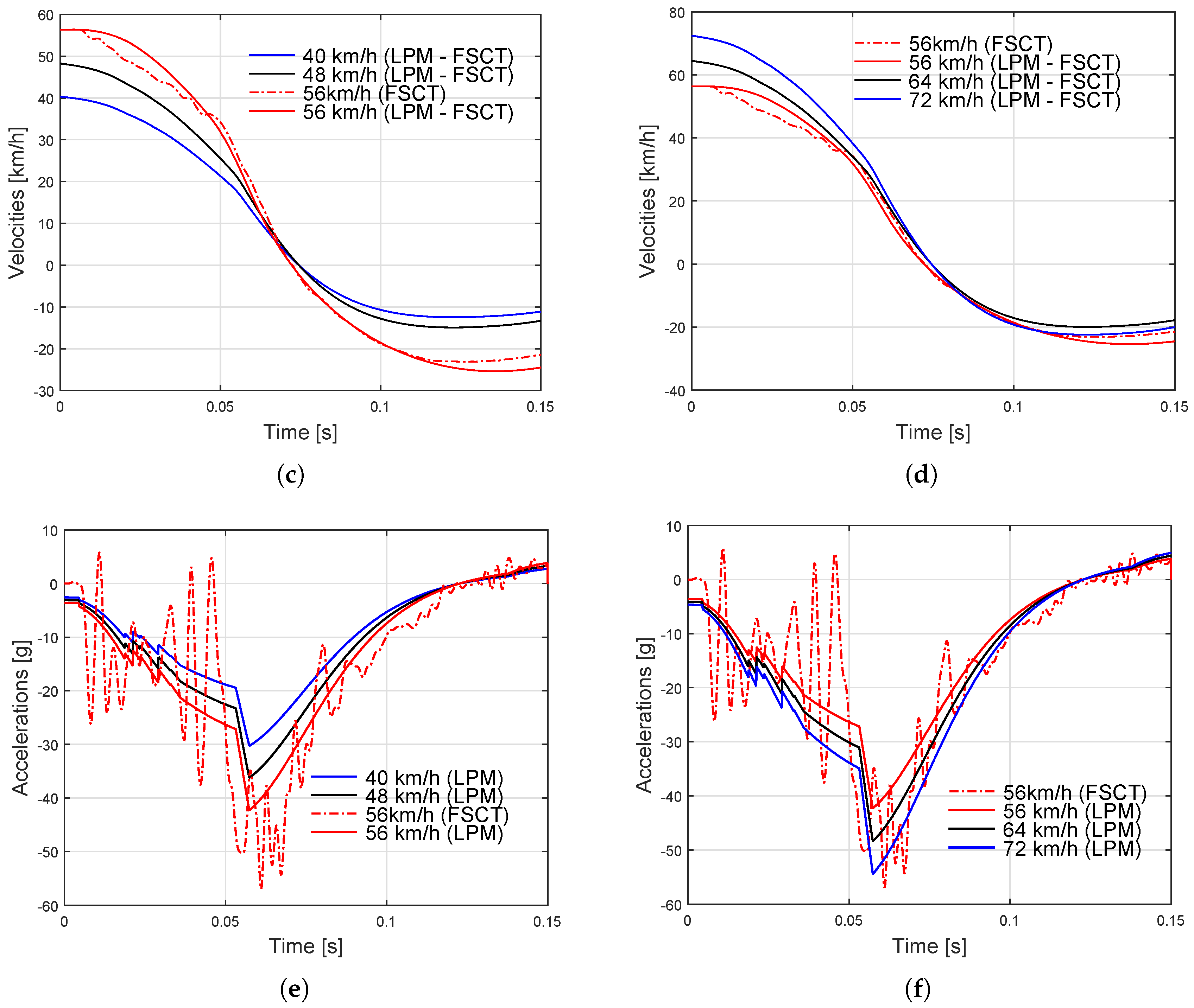
3. Results
4. Discussion
5. Conclusions and future work
Author Contributions
Funding
Conflicts of Interest
References
- European Standard EN 1317-1. Road Restraint Systems Part 1, Terminology and General Criteria For Test Methods; Technical Report; European Committee of Standardization: Brussels, Belgium, 2010. [Google Scholar]
- Pawlus, W.; Karimi, H.R.; Robbersmyr, K.G. Development of lumped-parameter mathematical models for a vehicle localized impact. J. Mech. Sci. Technol. 2011, 25, 1737–1747. [Google Scholar] [CrossRef] [Green Version]
- Kamal, M. Analysis and Simulation of Vehicle to Barrier Impact. SAE Int. Tech. Paper 1970, 1–6. [Google Scholar] [CrossRef]
- Marzbanrad, J.; Pahlavani, M. Calculation of vehicle-lumped model parameters considering occupant deceleration in frontal crash. Int. J. Crashworthiness 2011, 16, 439–455. [Google Scholar] [CrossRef]
- Marler, R.T.; Kim, C.H.; Arora, J.S. System identification of simplified crash models using multi-objective optimization. Comput. Methods Appl. Mech. Eng. 2006, 195, 4383–4395. [Google Scholar] [CrossRef]
- Kim, C.H.; Mijar, A.R.; Arora, J.S. Development of simplified models for design and optimization of automotive structures for crashworthiness. Struct. Multidiscip. Optim. 2001, 22, 307–321. [Google Scholar] [CrossRef]
- Huang, M. Vehicle Crash Mechanics, 1st ed.; CRC PRESS: Boca Raton, FL, USA, 2002. [Google Scholar]
- Pawlus, W.; Nielsen, J.E.; Karimi, H.R.; Robbersmyr, K.G. Application of viscoelastic hybrid models to vehicle crash simulation. Int. J. Crashworthiness 2011, 55, 369–378. [Google Scholar] [CrossRef]
- Alnaqi, A.; Yigit, A. Dynamic Analysis and Control of Automotive Occupant Restraint Systems. Jordan J. Mech. Ind. Eng. 2011, 5, 39–46. [Google Scholar]
- Klausen, A.; Tørdal, S.S.; Karimi, H.R.; Robbersmyr, K.G.; Jecmenica, M.; Melteig, O. Firefly Optimization and Mathematical Modeling of a Vehicle Crash Test Based on Single-Mass. J. Appl. Math. 2014, 1–10. [Google Scholar] [CrossRef]
- Klausen, A.; Tørdal, S.S.; Karimi, H.R.; Robbersmy, K.G. Mathematical Modeling and Numerical Optimization of Three Vehicle Crashes using a Single-Mass Lumped Parameter Model. In Proceedings of the 24th International Technical Conference on the Enhanced Safety of Vehicles (ESV), Gothenburg, Sweden, 8–11 June 2015; pp. 44–49. [Google Scholar]
- Ofochebe, S.M.; Ozoegwu, C.G.; Enibe, S.O. Performance evaluation of vehicle front structure in crash energy management using lumped mass spring system. Adv. Model. Simul. Eng. 2015, 2, 1–18. [Google Scholar] [CrossRef]
- Munyazikwiy, B.B.; Karimi, H.R.; Robbersmyr, K.G. A Mathematical Model for Vehicle-Occupant Frontal Crash using Genetic Algorithm. In Proceedings of the 2016 UKSim-AMSS 18th International Conference on Computer Modelling and Simulation, Cambridge, UK, 6–8 April 2016. [Google Scholar]
- Munyazikwiye, B.B.; Karimi, H.R.; Robbersmyr, K.G. Optimization of Vehicle-to-Vehicle Frontal Crash Model Based on Measured Data Using Genetic Algorithm. IEEE Access 2017, 5, 3131–3138. [Google Scholar] [CrossRef]
- Pahlavani, M.; Marzbanrad, J. Crashworthiness study of a full vehicle-lumped model using parameters optimization. Int. J. Crashworthiness 2015, 20, 573–591. [Google Scholar] [CrossRef]
- Lim, J.M. A Consideration on the Offset Frontal Impact Modeling Using Spring-Mass Model. Int. J. Mech. Aerosp. Ind. Mech. Manuf. Eng. 2015, 9, 1453–1458. [Google Scholar]
- Lim, J.M. Lumped Mass-Spring Model Construction for Crash Analysis using Full Frontal Impact Test Data. Int. J. Automot. Technol. 2017, 18, 463–472. [Google Scholar] [CrossRef]
- Mentzer, S.G. The SISAME-3D Program: Structural Crash Model Extraction And Simulation; Technical Report; US Department of Transportation: Washington, DC, USA, 2007.
- Mentzer, S.; Radwan, R.; Hollowel, W. The SISAME methodology for extraction of optimal lumped parameter structural crash models. SAE Tech. Paper 1992. [Google Scholar] [CrossRef]
- Gabler, H.C.; Hollowell, W.; Summers, S. Systems modeling of frontal crash compatibility. In Proceedings of the 2000 SAE International Congress and Exposition, Detroit, MI, USA, 13–15 January 2000; pp. 1–8. [Google Scholar]
- Mazurkiewicz, L.; Baranowski, P.; Karimi, H.R.; Damaziak, K.; Malachowski, J.; Muszynski, A.; Muszynski, A.; Robbersmyr, K.G.; Vangi, D. Improved child-resistant system for better side impact protection. Int. J. Adv. Manuf. Technol. 2018, 97, 3925–3935. [Google Scholar] [CrossRef] [Green Version]
- Vangi, D.; Cialdai, C.; Gulino, M.S.; Robbersmyr, K.G. Vehicle Accident Databases: Correctness Checks for Accident Kinematic Data. Designs 2018, 2, 4. [Google Scholar] [CrossRef] [Green Version]
- Sousa, L.; Verssimo, P.; Ambrosio, J. Development of generic multibody road vehicle models for crashworthiness. Multibody Syst. Dyn. 2008, 19, 133–158. [Google Scholar] [CrossRef]
- Teng, T.; Chang, F.; Liu, Y.; Peng, C. Analysis of dynamic response of vehicle occupant in frontal crash using multibody dynamics method. Math. Comput. Model. 2008, 48, 1724–1736. [Google Scholar] [CrossRef]
- Carvalho, M.; Ambrosio, J.; Eberhard, P. Identification of validated multibody vehicle models for crash analysis using a hybrid optimization procedure. Struct. Multidiscip. Optim. 2011, 44, 85–97. [Google Scholar] [CrossRef]
- Carvalho, M.; Ambrósio, J. Identification of multibody vehicle models for crash analysis using an optimization methodology. Multibody Syst. Dyn. 2010, 24, 325–345. [Google Scholar] [CrossRef]
- Ibrahim, H.K. Design Optimization of Vehicle Structures for Crashworthiness Improvement. Ph.D. Thesis, Concordia University, Montreal, QC, Canada, 2009. [Google Scholar]
- Mahmood, H.F.; Fileta, B.B. Vehicle Crashworthiness and Occupant Protection; Chapter 2; American Iron and Steel Institute: Washington, DC, USA, 2004; pp. 20–21. [Google Scholar]
- Deb, A.; Srinivas, K.C. Development of a new lumped-parameter model for vehicle side-impact safety simulation. J. Autom. Eng. 2008, 222, 1793–1811. [Google Scholar] [CrossRef]
- Piyush Dube, M.L.J.; Suman, V.B. Lumped Parameter Model for Design of Crash Energy Absorption Tubes. MSRUAS-SAS Tech. J. 2014, 13, 5–7. [Google Scholar]
- Ofochebe, S.; Enibe, S.; Ozoegwu, C. Absorbable energy monitoring scheme: new design protocol to test vehicle structural crashworthiness. Heliyon Elsevier 2016, 2, 1–33. [Google Scholar] [CrossRef] [PubMed]
- Tanlak, N.; Sonmez, F.; Senaltun, M. Shape optimization of bumper beams under high-velocity impact loads. Eng. Struct. 2015, 95, 49–60. [Google Scholar] [CrossRef]
- Lu, Q.; Karimi, H.R.; Robbersmyr, K.G. A Data-Based Approach for Modeling and Analysis of Vehicle Collision by LPV-ARMAX Models. J. Appl. Math. 2013, 2013, 1–10. [Google Scholar] [CrossRef]
- Prasad, P.; Padgaonkar, A.J. Static-to-Dynamic Amplification Factors for Use in Lumped-Mass Vehicle Crash Models. Soc. Autom. Eng. 1981, 1–43. [Google Scholar] [CrossRef]
- NHTSA. Vehicle Crash Test Database. 2016. Available online: http://www-nrd.nhtsa.dot.gov/database/vsr/veh/querytest.aspx (accessed on 25 May 2016).
- NHTSA. LS-DYNA FE Crash Simulation Vehicle Models. Available online: https://www.nhtsa.gov/crash-simulation-vehicle-models (accessed on 15 June 2016).
- Livermore Software Technology Corporation, Livermore, California 94551-0712. LS-DYNA Keyword User’s Manual, VOLUME II, Ls-Dyna R9.0 ed. 2016. Available online: https://www.dynamore.de/de/download/manuals/ls-dyna/ls-dyna-manual-r-9.0-vol-ii-16-mb (accessed on 24 October 2018).
- LSDYNA Supports. Available online: https://www.dynasupport.com/howtos/element/hourglass (accessed on 29 May 2018).
- European Standard EN 1317-2. Road Restraint Systems Part 2, Performance Classes, Impact Test Acceptance Criteria and Test Method for Safety Barriers Including Vehicle Parapets; Technical Report; European Committee of Standardization: Brussels, Belgium, 2010. [Google Scholar]
- Shojaat, M. Correlation between injury risk and impact severity index ASI. In Proceedings of the Swiss Transport Research Conference, Monte Verità/Ascona, Sweden, 20–22 March 2003. [Google Scholar]


| Parameters | LPM Calibrated to FSCT | LPM Calibrated to FEM |
|---|---|---|
| 7195 N/m | 25,718 N/m | |
| 7210 N/m | 31,444 N/m | |
| 25,386 N/m | 45,476 N/m | |
| 711,060 N/m | 467,830 N/m | |
| 0.0526 m | 0.2448 m | |
| 0.1023 m | 0.2923 m | |
| 59,444 Ns/m | 80,827 Ns/m | |
| 51,590 Ns/m | 7775 Ns/m | |
| 4997 Ns/m | 38,812 Ns/m | |
| 1382 Ns/m | 5703 Ns/m | |
| 7.0585 m/s | 4.7855 m/s | |
| 8.9272 m/s | 8.2880 m/s |
| Impact Velocities | ||||||
|---|---|---|---|---|---|---|
| Approaches | Parameters | 40 km/h | 48 km/h | 56 km/hc | 64 km/h | 72 km/h |
| FSCT | [s] | - | - | 0.0723 | - | - |
| [m] | - | - | 0.7551 | - | - | |
| ASI [-] | - | - | 2.5 | - | - | |
| LPM calibrated to FSCT | [s] | 0.0736 | 0.0740 | 0.0738 | 0.0741 | 0.0741 |
| [m] | 0.5373 | 0.6429 | 0.7508 | 0.8588 | 0.9653 | |
| ASI [-] | 1.7 | 2.1 | 2.6 | 2.7 | 3.1 | |
| FEA | [s] | 0.0755 | 0.0781 | 0.0801 | 0.0804 | 0.0800 |
| [m] | 0.5077 | 0.6077 | 0.7180 | 0.8331 | 0.9408 | |
| ASI [-] | 1.5 | 1.8 | 2.0 | 2.3 | 2.5 | |
| LPM calibrated to FEA | [s] | 0.0824 | 0.0825 | 0.0793 | 0.0822 | 0.0805 |
| [m] | 0.5231 | 0.6258 | 0.7108 | 0.8360 | 0.9396 | |
| ASI [-] | 1.4 | 1.6 | 2.0 | 2.3 | 2.5 | |
© 2018 by the authors. Licensee MDPI, Basel, Switzerland. This article is an open access article distributed under the terms and conditions of the Creative Commons Attribution (CC BY) license (http://creativecommons.org/licenses/by/4.0/).
Share and Cite
B. Munyazikwiye, B.; Vysochinskiy, D.; Khadyko, M.; G. Robbersmyr, K. Prediction of Vehicle Crashworthiness Parameters Using Piecewise Lumped Parameters and Finite Element Models. Designs 2018, 2, 43. https://doi.org/10.3390/designs2040043
B. Munyazikwiye B, Vysochinskiy D, Khadyko M, G. Robbersmyr K. Prediction of Vehicle Crashworthiness Parameters Using Piecewise Lumped Parameters and Finite Element Models. Designs. 2018; 2(4):43. https://doi.org/10.3390/designs2040043
Chicago/Turabian StyleB. Munyazikwiye, Bernard, Dmitry Vysochinskiy, Mikhail Khadyko, and Kjell G. Robbersmyr. 2018. "Prediction of Vehicle Crashworthiness Parameters Using Piecewise Lumped Parameters and Finite Element Models" Designs 2, no. 4: 43. https://doi.org/10.3390/designs2040043
APA StyleB. Munyazikwiye, B., Vysochinskiy, D., Khadyko, M., & G. Robbersmyr, K. (2018). Prediction of Vehicle Crashworthiness Parameters Using Piecewise Lumped Parameters and Finite Element Models. Designs, 2(4), 43. https://doi.org/10.3390/designs2040043