Abstract
Structural system design is the process of giving form to a set of interconnected components subjected to loads and design constraints while navigating a complex design space. While safe designs are relatively easy to develop, optimal designs are not. Modern computational optimization approaches employ population based metaheuristic algorithms to overcome challenges with the system design optimization landscape. However, the choice of the initial population, or ground structure, can have an outsized impact on the resulting optimization. This paper presents a new method of generating such ground structures, using a combination of topology optimization (TO) and a novel system extraction algorithm. Since TO generates monolithic structures, rather than systems, its use for structural system design and optimization has been limited. In this paper, truss systems are extracted from topologies through morphological analysis and artificial intelligence techniques. This algorithm, and its assessment, constitutes the key contribution of this paper. The structural systems obtained are compared with ground truth solutions to evaluate the performance of the algorithms. The generated structures are also compared against benchmark designs from the literature. The results indicate that the presented truss generation algorithm produces structures comparable to those generated through metaheuristic optimization, while mitigating the need for assumptions about initial ground structures.
1. Introduction
The conventional structural design process centers around the use of design requirements and constraints to choose a single efficient structure from the large decision space of all possible designs, all the while working with time and budget limitations. The structural design space has been shown to be typically comprised of local optima, resulting in non-convex optimizations [1,2], and with solutions often dependent upon specified initial conditions [3]. Compounding the problem, structures are generally composed of a system of components, and so the performance and efficiency of any design is governed by a combination of the system topology and the design of each component as well. Thus, the design space for any set of design criteria can be extremely large.
Modern computational approaches for determining efficient structural designs often use a metaheuristic, such as evolutionary computation, to obtain an optimal solution. Such metaheuristic approaches are typically initialized via a ground structure approach, in which an assumed structural system configuration serves as an initial sample population [4,5]. This paper presents a new method of generating such ground structures automatically, using a combination of topology optimization (TO) and a novel system extraction algorithm.
1.1. Literature Review
The overall methodology for design optimization in the literature primarily revolves around initializing the optimization problem with initial structural assemblies and iteratively improving them, resulting in an optimal structure. Reference [6] presented a method for discrete optimization of structural assemblies using genetic algorithms. The structure was treated as a collection of nodes interconnected via structural members. Reference [7] used the ground structure approach for truss topology optimization. Similar methods of structural optimization using the ground structure approach have been applied to diverse problems [2,3,4] using various algorithms [5,8,9,10,11]. Furthermore, with improved optimization heuristics and higher computation capabilities, optimization has been performed for complex structures. However, the key drawback to such approaches is that the final optimal design is dependent on the initial structural systems selected for optimization [1,3] and a poorly chosen ground structure may lead to suboptimal designs.
Topology optimization (TO), the process of finding the optimal layout (topology) of a structure, requires fewer assumptions about the design domain compared to metaheuristic approaches. Two of the most established TO approaches are density based methods and hard kill methods. Density based methods discretize the design domain into a mesh and optimize the design by varying the density of each element of the mesh based on an objective function. Fundamentally, this is a challenging large-scale integer programming problem. In order to simplify the TO problem and express it as a function of continuous design variables, an interpolation function with a penalization mechanism is generally used. Different penalization and interpolation methods lead to different algorithms for TO such as Solid Isotropic Material with Penalization (SIMP) [12,13], Rational Approximation of Material Properties (RAMP) [14] and SINH (not an acronym) [15]. A detailed discussion of the SIMP approach, including implementation issues, can be found in [16]. For a review of the recent developments in SIMP, the reader is referred to [17,18]. Research has also been conducted in using TO with material failure constraints [19] and stress constraints [20]. TO has been widely used in different domains such as fluid flow [21], heat transfer [22] and aerospace design [23,24]. Hard kill methods gradually remove (or add) material from the design based on a heuristic strategy, with Evolutionary Structural Optimization (ESO), developed by [25], as the most well known of such methods. In this research, solid isotropic material with penalization (SIMP) was implemented due to its widespread usage [17] and the chaotic convergence behavior of Evolutionary Structural Optimization (ESO) [26].
1.2. Contribution of This Research
As stated, a critical aspect of metaheuristic design optimization is the choice of ground structure that serves as the initial population for optimization. Selecting such ground structures requires implicit assumptions about the location of those structures in the design landscape. As such, there is a need for methods to generate such structures automatically, without strong assumptions about the design landscape.
Topology optimization presents an avenue for addressing this need. However, regardless of the specific method used, topology optimization results in monolithic structures, rather than the systems of engineered components that comprise the majority of structural designs. This is a critical limitation, as it inhibits topology optimization from being used to either generate initial structures for further optimization, or for generating structural designs in many practical scenarios.
Presented in this paper is a new algorithm to generating structural systems, in the context of truss design. This algorithm extracts structural systems from generated topologies, which can either be analyzed directly or serve as the initial ground structures for further optimization. The extraction is accomplished through a combination of morphological analysis and artificial intelligence techniques. This system extraction approach, and its evaluation, constitutes the primary contribution of this work.
In this manuscript, the complete system extraction methodology is first presented. This is followed by a study on the behavior of systems manually extracted from monolithic structural topologies. The performance of three automatic extraction algorithm variants is then evaluated. A sensitivity study of algorithm performance is included as well.
2. Methodology
The system generation process starts with a given design domain and the initial conditions necessary to support topology optimization. A system topology is then generated through topology optimization, based on these inputs (Section 2.1). Nodes and structural elements are extracted from this topology through a combination of morphological analysis and associated computational techniques (Section 2.2), yielding a structural assembly (system). The extracted structural assembly can then be analyzed using finite element analysis to perform structural analysis to obtain the deflections and member stresses. This assembly can also serve as a basis for structural optimization. An overview of the process is provided in Figure 1.
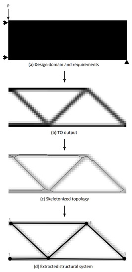
Figure 1.
Desired representation of a TO structure for structural optimization.
2.1. Topology Optimization
While any number of topology generation approaches can be used as part of the overall methodology, in this work, the SIMP density-method is used due to its consistent performance across a range of application scenarios [26]. Reference [27] first presented this approach for generating optimal topologies in structural design using numerical optimization and homogenization methods. The objective of their optimization was to minimize the work done by applied loads as shown in Equation (1).
In Equation (1), is the elasticity matrix, is the energy in bilinear form i.e., the internal virtual work of an elastic body at equilibrium and for an arbitrary virtual displacement , represents the load linear form of the energy, and are body and boundary forces, represents the linearized strain in each direction. Thus, this formulation minimizes the strain energy, while limiting the displacements as per the imposed design constraints and the admissible displacements (U):
The design space of the problem is defined as , the strain as , and the indicator function χ indicates whether material is present at a point x or not. Hence, for all , either or i.e., at any point in the domain, either material is present or it is not. This formulation also assumes that the material is linearly elastic. For example, in Figure 1a, the black rectangle is the design domain, , with the black color throughout the design domain indicating that everywhere. As the design is optimized, the design domain remains the same but the location of material in the domain changes, resulting in Figure 1b. The elasticity matrix for the material is therefore defined as at any location .
This optimization problem can be modeled as a large scale integer programming problem and is generally ill posed and difficult to solve [16]. Reference [12] modified the problem by replacing the indicator function with a density function, that is continuous between 0 and 1, rather than binary. The modified elasticity matrix is . The density function transforms the problem from a large scale integer optimization problem to an easier to handle continuous problem. Since the desired density value is either 0 or 1, constraints are imposed via penalization. This penalization supplies the name of this approach: solid isotropic material with penalization (SIMP). The definition of is further modified and it is redefined as:
Choosing makes the densities between 0 and 1 unfavorable since, for the same amount of material, it provides a lesser stiffness due to the exponent p. In general, in order to obtain solutions with minimal volumes with intermediate densities, or binary designs, it is recommended to use p ≥ 3. Once the problem has been thus formulated, the density of the material within the design space is optimized. The design at each iteration is analyzed through finite element analysis where each region with a density value corresponds to an element. The value of the objective function is thus computed. Based on the objective function, the topology is iteratively updated to yield a new topology until the termination criteria are satisfied.
Since SIMP treats the topology optimization problem as essentially a material redistribution problem, all resulting topologies are monolithic structures, rather than structural systems of interconnected components. The second part of the presented computational process is designed to extract such systems directly from the topologies.
2.2. Node-Element Extraction from Topologies
After a topology is obtained, the next step is to convert it into a system consisting of nodes (joints) and connecting elements to suit structural engineering purposes. The morphological skeleton of the topology, as well as branch and end points in that skeleton, are first found. The skeleton is then further analyzed using one of the three variants of a node-element identification algorithm (NEI) developed in this study (Figure 1). The first algorithm, NEI-CL (Section 2.2.2), is based on clustering directional vectors that initiate at a given node and terminate at discretized locations throughout the topology. The second algorithm, NEI-HLT (Section 2.2.3), uses Hough transform line-finding to identify components [28]. The third algorithm, NEI-TRA (Section 2.2.4), is based on the concept of a structural component as a path between nodes such that there is no other node along this path. Therefore, given the location of nodes, this algorithm traverses from one node to another and identifies the connectivity between nodes.
2.2.1. Topology Skeletonization
The first step in identifying nodes and elements is to convert the generated topology into a binarized and discretized representation, analogous to a black and white image. The binarization is performed using Otsu’s method [29]. The skeleton of the topology is then determined via morphological thinning of the binarized topology [30]. The branch points and end points of the skeleton are detected automatically by analyzing the 8-connectivity of the skeleton, yielding the potential nodes of the structure. However, it is important to note that this method of identifying nodes does not necessarily yield all of the correct nodes in some cases because of approximations in the skeletonization process. Evidence of this effect will be shown in later analyses.
2.2.2. NEI-CL: Directional Clustering Algorithm Variant
For the NEI-CL algorithm variant, the direction vectors from each node to each pixel in the skeleton, within a specified distance from the node, are calculated. These vectors are clustered together for each node using k-means clustering [31], with each cluster of vectors corresponding to a potential structural element. Any two nodes with a clustered set of direction vectors oriented towards each other are matched and identified as nodes and endpoints of a potential element. Structural elements are then identified along each cluster’s direction vector, and the endpoints of these elements are labeled as nodes.
This process occasionally results in multiple, and closely spaced, nodes at the ends of identified elements. As a post-processing step, the set of nodes is clustered, again via the k-nearest neighbors algorithm, to remove closely spaced and potentially duplicate nodes. Potential elements are also evaluated for duplicates. Finally, all nodes without any connected elements are removed, yielding the final set of nodes and elements. The pseudo code for this algorithm is shown in Figure 2.
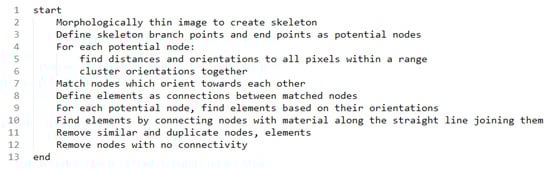
Figure 2.
Pseudo code for the NEI-CL algorithm.
2.2.3. NEI-HLT: Hough Line Transform Based Algorithm Variant
As with the NEI-CL algorithm, the topology is first converted into a morphological skeleton, and branch and endpoints are determined. The Hough transform [28,30], a well-established method for finding line segments in images, is then applied. Given the assumption that all structural elements will connect between nodes in a straight line, lines found through the Hough transform are labeled as candidate structural elements. Duplicate endpoints of lines are merged using k-means clustering and line segments with similar directionality and endpoints are joined to form a single element. The pseudo code for this algorithm is shown in Figure 3.
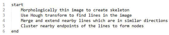
Figure 3.
Pseudo code for the NEI-HLT algorithm.
2.2.4. NEI-TRA: Node to Node Traversal Algorithm Variant
The NEI-TRA algorithm variant iteratively traverses each segment initiating from each potential node of the skeleton and stores the coordinates of each pixel in the traversal. The traversal, starting from a node, proceeds by repeatedly moving from one pixel to another pixel in its 8 point neighborhood. Once another identified node is reached and the traversal is complete, the goodness of fit of a line connecting the two nodes is evaluated against the traversed pixels. The goodness of fit is evaluated by using the coefficient of correlation and checking if all the traversed pixels fall within a specified bandwidth from the line. If the fit is good, then an element is assigned between the two nodes. In Figure 4a, the pixels from traversal along the segments 1, 2 and 3 have a good fit with the straight lines connecting the nodes. If the fit is not good (Figure 4a, segment 4), then the set of pixels is divided into subsegments of the skeleton of a specified length (Figure 4b) and the average direction vector is computed for each subsegment. The direction vectors are then clustered so that subsegments with similar direction vectors together are part of the same cluster. Subsegments in each cluster constitute an element. Figure 4c shows a sample in which the subsegments have been clustered to yield elements. If the endpoints of this element are not already present in the potential nodes, they are added as additional nodes. Lastly, similar and duplicate nodes and elements are removed through k-means clustering to obtain the final set of nodes and elements. The pseudo code for the NEI-TRA algorithm is shown in Figure 5.
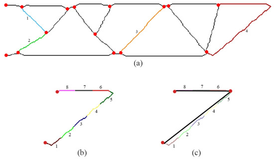
Figure 4.
Cluster based element identification in NEI-TRA algorithm. (a) segments connecting branch points; (b) subsegments for identifying elements from the segment; (c) elements identified after clustering.
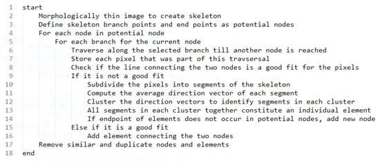
Figure 5.
Pseudo code for the NEI-TRA algorithm.
3. Experiments and Results
This section presents and discusses the results of experiments designed to evaluate the suitability of TO for generating structural systems. First, truss systems manually extracted from topologies were compared against benchmark optimization solutions in the literature, in order to better understand the nature of systems extracted from topologies. The three automatic system extraction variants were then comparatively analyzed. A parameter sensitivity study of the NEI-TRA algorithm variant was then performed, as this variant produced the most consistent results.
3.1. Preliminary Analysis: Extracting Structural Systems from Topologies
In this study, the design constraints for two established problems from the structural optimization literature were used as a basis for TO. Structural systems were then manually extracted from the topologies, and the performance of these systems was compared against benchmark optimized solutions from the literature. This study was performed in order to validate the initial idea of generating structural systems using TO. The design problems shown in Figure 6a and Figure 7a were used as input for TO, and extracted systems were compared with the results published by [4,10,32,33,34]. It is important to clarify that the solutions in these previous works were obtained by starting from an initial structural system, and iteratively optimized by adding members, removing members and, in some cases, modifying node locations. These variations to the structure were introduced as per optimization heuristics such as a genetic algorithm, particle swarm optimization, or differential evolution.
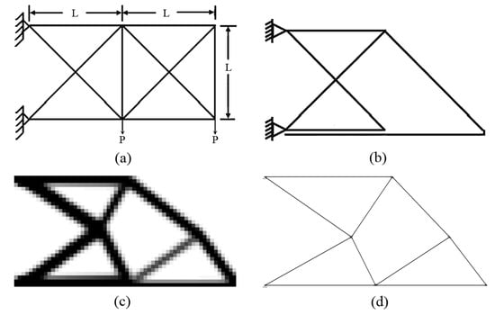
Figure 6.
(a) initial structure for prior solutions to Problem 1 [10]; (b) optimal solution from [10]; and (c) TO solution; and (d) TO solution converted to a truss.
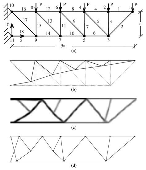
Figure 7.
(a) initial structure for prior solutions to Problem 2; (b) optimal solution from [34]; (c) TO solution; and (d) TO solution converted to truss. Note the additional members needed for stability.
For the first design domain, “Problem 1”, a design space 18.288 m (720 inches) wide and 9.144 m (360 inches) high with two loads, each p = −4444.82 kN (−100 kips), was specified. A design space 31.75 m (1250 inches) wide and 6.35 m (250 inches) high with 5 point loads, each p = −88.96 kN (−20 kips), acting on it was specified for “Problem 2”. Both problems used aluminum with a 69 GPa modulus of elasticity as the structural material. Loads and boundary conditions were applied as per Figure 6a and Figure 7a. Topologies were generated using a modified version of Sigmund’s 99 line Matlab code for SIMP [35]. Each structure was converted to a truss system by manually identifying nodes and elements, and adding extra members if needed for stability. The results obtained were then imported into Risa [36] for evaluation. The designs reported in the literature were also simultaneously evaluated in Risa 2D.
SIMP requires a volume fraction parameter, a parameter that determines the fraction of the volume of the design domain that will contain material. Several volume fractions were tested and it was observed that higher volume fractions increased the weight of the structure and reduced the deflections and member stresses, as is to be expected. For both problems, a volume fraction was eventually selected that generated design weights comparable to prior efforts. Since the objective function of SIMP topology optimization is evaluated via finite element analysis, parameters for discretization of the design domain such as the number of elements needs to be specified. The impact of the fineness of the discretization has been well documented in the TO literature [16], and is not studied here. The resolutions of the meshes were determined empirically as 60 × 30 for Problem 1 and 175 × 35 for Problem 2, and were selected due to the consistency of topologies generated in a range of resolutions centered on these values.
3.1.1. Metrics
As the volume fraction was iteratively changed to match previous design weights, the structural weight was not useful as a comparative metric. Instead, the average stress, maximum stress, and maximum deflection were used for comparisons.
3.1.2. Results
For Problem 1, the volume ratio was specified as 0.2. With regards to the compared studies, References [4,32] only varied the cross-sectional area of the initial structure but did not add or remove members. Reference [10] presented a solution with no removal of members and another solution in which removal of structural members was permitted. A comparison of the weight, deflection, maximum stress and average stress is shown in Table 1.

Table 1.
Comparative results for Problem 1.
The structure optimized by [10], which permitted member removal, was 5.8% lighter than the other structures, which all had very similar weights. The TO-based truss was the heaviest, and had slightly higher deflections. The TO-based results reflect a maximum stress of 58.0 MPa and an average stress of 49.8 MPa, which is a notably more even stress distribution than the other structures. It is assumed that, given additional optimization, the TO-based system would converge to a solution similar to those of prior efforts.
The TO solution to Problem 2 was compared with the designs published in [33,34]. In both of these studies, an initial structure was assumed for optimization. The node locations could be modified, but member removal was not permissible. The area of cross-section of the members could also be modified to optimize the structure. For the topology optimization, the volume ratio was set to 0.2.
TO resulted in structures that were unstable when directly converted to trusses, a problem not encountered in Problem 1. Hence, the structure was first evaluated as a frame with complete joint fixity. Members were then manually added to this frame for stability, and it was converted to a truss with pin supports (Figure 7d). A comparison of the results is shown in Table 2.
Table 2.
Comparative results for Problem 2.
Table 2 shows that the structures optimized in the literature are lighter than the TO designed structures by about 2% for the frame structure and 6.7% for the truss structure. However, the TO structure has slightly lower maximum stresses, lesser average stress and significantly lower deflections. The deflection of the TO truss structure is less than half the deflection of the structures optimized by [33,34]. In addition, the variation in the member stresses is 13.6% lesser for the TO truss structure and 33.6% lesser for the TO frame structure, which indicates a more evenly distributed load in the TO structure. This is similar to the results of Problem 1.
What the results of this analysis illustrate is that systems extracted from structural topologies can perform comparably to systems optimized assuming an initial structural configuration. This is particularly true given that the extracted systems could be further optimized using any number of established techniques. Therefore, generating a topology and then extracting a system from it can serve as a full replacement for an initial estimate of a structural configuration. In such cases, the specified volume ratio becomes the controlling design parameter. It is also important to recognize that, as shown by Problem 2, topology optimization results can require some post-processing in order to generate stable results.
3.2. Extraction Algorithm Analysis
In the preliminary analysis, systems were manually extracted from topologies. The three automatic extraction algorithms designed to address this issue are analyzed in this section. Four diverse topologies (TO1, TO2, TO3, TO4) were generated and used for testing (Figure 8). These topologies have variations in member thickness, number of members, and general topological complexities that illustrate both the capabilities and limitations of the extraction process. A ground truth extraction solution was developed based on manual labeling of nodes and elements in the TO structure. After evaluating the three variants, a parameter sensitivity analysis was conducted for NEI-TRA, as it produced the most consistent results.
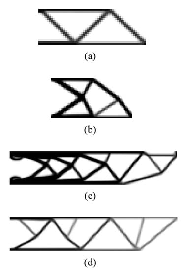
Figure 8.
TO structures used as inputs for algorithm to identify nodes and elements.
3.2.1. Metrics
Fundamentally, the performance of each algorithm was evaluated based on how accurately it identified nodes and elements. Since the nodes in a TO structure are not visually distinct as a single point, but, as a region, identifying the exact ground truth node location is subjective. In order to capture this subjectivity, and to determine the most likely node location, the labeling of the nodes was performed by twenty individuals. The marked locations were then averaged to yield the ground truth. A standard deviation indicating the variation in individual marking of node locations was also computed (termed as “node location variance”). This node location variance quantified the subjectivity of the node identification in the ground truth itself and, as will be shown, correlated with the ability of the extraction algorithms to properly segment the structures. The node location variance is illustrated as green circles (radius is proportional to the variance) in Figure 9d, Figure 10d, Figure 11d and Figure 12d.
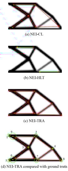
Figure 9.
Node and element identification results for TO1.
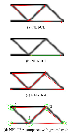
Figure 10.
Node and element identification results for TO2.
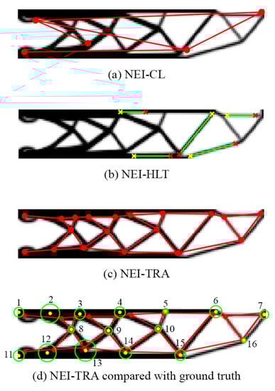
Figure 11.
Node and element identification results for TO3.
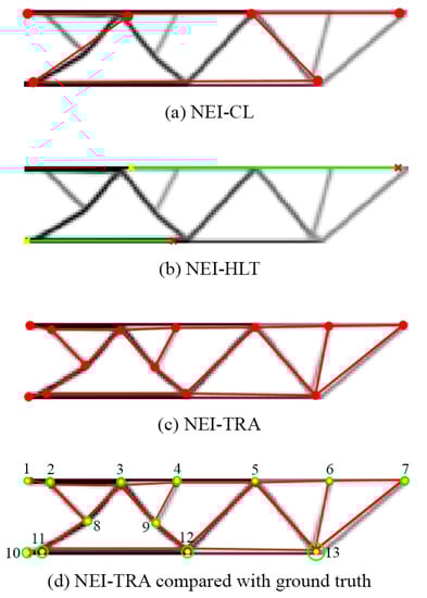
Figure 12.
Node and element identification results for TO4.
3.2.2. Results
The results for TO1 are shown in Figure 9. A visual examination clearly shows that the traversal based algorithm (NEI-TRA) outperforms the other two algorithms. As shown in Table 3, the cluster based algorithm (NEI-CL) (Figure 9a) was unable to identify three of the elements. The Hough line transform based algorithm (NEI-HLT) only identified two elements out of a total of ten elements (Figure 9b). The reason for this poor performance is that the Hough line transform uses the skeleton to identify straight segments. Approximations in the skeleton in the form of curves result in the Hough transform being unable to detect lines. Hence, in skeletons obtained from poorly defined or curved topologies, the performance of the Hough line transform is poor. With regards to NEI-TRA (Figure 9c), there is a slight oversegmentation of one element and it thus identifies 13 elements instead of 10.
Table 3.
Number of nodes and elements identified by different algorithms.
Multiple nodes were identified at some joints since the analysis of the morphological skeleton occasionally yielded closely spaced branch points (see Figure 4a for closely spaced branch points). It is worth noting that 40% of the manual ground truth sets indicated two nodes as well, similar to what the algorithm indicated. For the nodes with more node location variance in the ground truth (1, 6, 8 and 9), the algorithm results were a little farther from the ground truth. The NEI-TRA algorithm detected all the elements of the structure.
The performance of the three algorithms for TO2 is shown in Figure 10 and Table 3. The NEI-CL algorithm detected all but two elements and identified a majority of the nodes in the structure. The NEI-HLT algorithm, on the other hand, detected only one element again due to approximations in skeletonization. The NEI-TRA algorithm identified all the elements and nodes. However, due to the skeleton’s structure, additional nodes were detected as seen with TO1.
A comparison with the ground truth (Figure 10d) showed that the performance of the NEI-TRA algorithm was superior. It identified the nodes accurately in all cases. Multiple nodes along with an extra element were detected at two joints in the structure due to the skeleton having multiple branch points in the vicinity of that joint. The algorithm correctly detected only one node in the top left corner, whereas 50% of the ground truth labels had two nodes at this joint.
The nodes and elements identified by each of the algorithms for TO3 are shown in Figure 11. The NEI-TRA algorithm outperforms the other two variants in this case as well. The NEI-CL algorithm performed relatively poorly due to the increased amount of material in this structure (as a result of a higher volume ratio). The algorithm erroneously identified elements which do not exist as a result. The NEI-HLT algorithm also performed poorly, with only a few elements being detected due to approximations in the skeleton. The NEI-TRA algorithm provided the most reasonable system again with a slight oversegmentation.
Comparing with the ground truth, the NEI-TRA algorithm again shows multiple nodes at some joints (Figure 11d) due to the skeleton containing multiple branch points in those locations. Nodes with more variance in the ground truth labeling, such as nodes 2 and 12, had more distance between the ground truth node and algorithm identified node (see Table 4). In contrast, node 13 is accurately identified although the variance in the ground truth was high for this node. It is worth noting that noticeable errors were obtained at the leftmost nodes of the structure (nodes 1 and 11) since the skeleton endpoint is not exactly at the actual structure support location.
Table 4.
Evaluating the NEI-TRA algorithm performance against the ground truth node coordinates.
Figure 12 shows the nodes and elements identified by the three algorithms for TO4 structure. The results show that the NEI-TRA algorithm was again the best performer. The NEI-HLT algorithm showed the poorest performance due to skeleton approximations. The NEI-CL algorithm detected about half of the elements in the structure. The nodes detected were, however, very close to the actual node locations from the benchmark solutions.
Since this topology’s elements have less thickness, the skeleton of the structure is a very good representation of the actual structure. As a result, the NEI-TRA algorithm detects nodes and elements very accurately. Quantitatively, it can be seen that the mean error in node location for TO4 was much lower than the node location error for all other structures tested (Table 5). Hence, the solution obtained using the traversal based algorithm is very close to the ground truth solution (Figure 12d).
Table 5.
Geometric accuracy of the NEI-TRA algorithm.
3.2.3. Summary
This analysis showed that the NEI-TRA algorithm, based on depth first search traversal and k-means clustering, clearly demonstrated superior performance compared to the NEI-CL and NEI-HLT algorithms. NEI-HLT performs poorly due to approximations in skeletonization. NEI-CL identifies erroneous direction vector clusters as elements leading to falsely identified elements. This erroneous identification of clusters is a classic problem of separating signal (clusters that are actual elements) from the noise (clusters that are not elements). The NEI-TRA algorithm demonstrated a better performance since its conceptual assumptions that nodes are branch points in skeleton and that nodes are connected via lines in the skeleton, do not have a signal and noise separation problems as severe as the other two algorithms. Upon identifying the NEI-TRA algorithm as the best approach, a sensitivity analysis was performed, which is presented in the next section.
3.3. Sensitivity Analysis
The NEI-TRA algorithm has five controlling parameters. A bandwidth parameter, “α”, is used to check if the line connecting two nodes is a good fit for the pixels (Figure 5, line 8). Three parameters are used for clustering nodes in order to eliminate similar nodes (Figure 5, line 17): a cluster standard deviation parameter and two inter-nodal distance parameters. A second bandwidth parameter “β” is used for removing redundant elements and breaking up long elements into smaller elements if the required criteria are met (Figure 5, line 17). The effect of each parameter is explored in greater depth in this section.
3.3.1. Impact of Bandwidth Parameter α
Six different values of the bandwidth parameter α, from 2 pixels to 12 pixels, were tested. In the results shown, an α value of 4 was used. It was observed that the impact of this parameter on the resulting system is not significant since the main purpose of this parameter is to make the algorithm faster. Once the pixels from the traversal are determined, there are two ways of processing it. If the line connecting the end point nodes is a good fit, which is true if no pixel is more than α pixels away from a line, then an element connecting the nodes is added (Figure 5, line 15–16). If the fit is not good, then a clustering approach is used (Figure 5, line 9–14). If α is too small, then the clustering approach is used more frequently resulting in a slower runtime. Furthermore, the clustering approach can determine different endpoints from the existing nodes and hence create additional nodes. However, after removing similar nodes, the final nodes and elements obtained did not change significantly as seen for TO3 (Figure 13a).
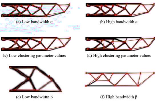
Figure 13.
Impact of different parameters on the performance of the NEI-TRA algorithm.
3.3.2. Impact of the Three Clustering Parameters
In order to remove redundant nodes, clustering is used (Figure 5, line 17). Three parameters together control this clustering. Fifteen combinations of these parameters, with settings varying from 5 pixels to 30 pixels, were evaluated. Small values for these parameters cluster only the nodes that are very close to each other, whereas larger values can cluster nodes that are farther apart spatially. This can be seen in Figure 13d, where higher values of these parameters cluster nearby nodes. For TO3, the impact was most noticeable since nodes are relatively close to each other. Hence, higher values of this parameter ended up clustering non redundant nodes, which should not be clustered into one node. The best results were obtained with the three parameters having values of 10, 15 and 7.5.
3.3.3. Impact of Bandwidth Parameter β
Redundant elements are removed and long elements are broken into appropriate smaller elements using the control parameter β. For example, the top elements in Figure 13f, which connect the leftmost top node to the rightmost top node are formed by breaking a long element that connects the leftmost and rightmost nodes into multiple smaller elements with intermediate nodes. Ten β values ranging from 5 pixels to 50 pixels were tested for this sensitivity analysis. If the value of the parameter was too large (more than 40 pixels), then the element was erroneously segmented as shown in Figure 13f. Similarly erroneous segmentations were seen in the other topologies as well. If the parameter was too small (10 pixels or less), then some redundancy in elements persisted as illustrated for TO1 in Figure 13e. A β value of 20 resulted in the most consistent element identification.
4. Conclusions
This paper presents a new method of generating structural systems using a combination of topology optimization and an automated algorithm for extracting systems from a topology. The benefits of this approach are that, compared to other approaches to structural optimization, it does not require an assumed structural system for initiation. Instead, broader constraints such as loadings, geometric boundaries, and volume ratios are required instead.
From a practical perspective, the presented method has several potential applications. The first is that the generated systems can be used as the initial population for metaheuristic optimization, mitigating the need for assumptions about the topology of these initial ground structures. Another application would be to incorporate the system generation algorithm into a software program that provides a set of structure prototypes for an engineering team to consider a more detailed design, improving the efficiency of the overall design process.
From the preliminary TO system study, several conclusions can be drawn. One of the foremost observations is that structural systems derived manually through TO are efficient and comparable to optimal structures from the literature in most cases. These systems were comparable with respect to deflections. The TO-based systems resulted in more balanced member stresses compared to the benchmark solutions, which had members with very high and very low stresses. In some cases, however, the system extracted from the topology was not stable for a truss configuration, requiring manual post-processing.
Once the viability of using TO for deriving systems was verified, the three extraction algorithms were tested. The NEI-TRA algorithm demonstrated the most consistent performance and accurately identified the most nodes and elements across different scenarios. A key aspect of the extraction process presented here is the analysis of the morphological skeleton to identify nodes and their connectivity. Hence, the algorithm performs well in scenarios where the skeleton of the structure is a close representation of the actual structure. In situations where this does not hold, the performance of the algorithm deteriorates. This was clearly seen in cases where the skeletonization process was modified to yield a skeleton unrepresentative of the actual structure. The algorithm itself is dependent on several parameters. The best performance was seen when the values of the bandwidth α was 4, β was 20 and the three clustering parameter values were between 7.5 and 15. The values of these parameters will change depending on the scale of the input for the algorithms. Higher resolution inputs to the algorithm will need larger parameter values and vice versa.
One persistent issue with the NEI-TRA algorithm was the multi-node problem wherein multiple nodes were detected instead of a single node. Further research is required to remedy this issue. Another avenue for future work is to use additional structural optimization to further improve the designs generated through the topology extraction process.
Author Contributions
Achyuthan Jootoo and David Lattanzi conceived and designed the experiments. Achyuthan Jootoo developed the algorithms and programs, performed the experiments, and analyzed the data. Achyuthan Jootoo wrote the paper with reviews, and significant inputs and edits were completed by David Lattanzi.
Conflicts of Interest
The authors declare no conflict of interest.
Abbreviations
The following abbreviations are used in this manuscript:
| TO | Topology Optimization |
| EA | Evolutionary Algorithms |
| SIMP | Solid Isotropic Material with Penalization |
| NEI-CL | Node Element identification via Clustering |
| NEI-HLT | Node Element identification via Hough Line Transform |
| NEI-TRA | Node Element identification via Node to Node Traversal |
References
- Rajan, S.D. Sizing, Shape, and Topology Design Optimization of Trusses Using Genetic Algorithm. J. Struct. Eng. 1995, 121, 1480–1487. [Google Scholar] [CrossRef]
- Ho-Huu, V.; Vo-Duy, T.; Luu-Van, T.; Le-Anh, L.; Nguyen-Thoi, T. Optimal design of truss structures with frequency constraints using improved differential evolution algorithm based on an adaptive mutation scheme. Autom. Constr. 2016, 68, 81–94. [Google Scholar] [CrossRef]
- Kicinger, R.; Arciszewski, T.; DeJong, K. Evolutionary Design of Steel Structures in Tall Buildings. J. Comput. Civ. Eng. 2005, 19, 223–238. [Google Scholar] [CrossRef]
- Xu, T.; Zuo, W.; Xu, T.; Song, G.; Li, R. An adaptive reanalysis method for genetic algorithm with application to fast truss optimization. Acta Mech. Sin. 2009, 26, 225–234. [Google Scholar] [CrossRef]
- Tejani, G.G.; Savsani, V.J.; Bureerat, S.; Patel, V.K. Topology and Size Optimization of Trusses with Static and Dynamic Bounds by Modified Symbiotic Organisms Search. J. Comput. Civ. Eng. 2017, 32, 04017085. [Google Scholar] [CrossRef]
- Rajeev, S.; Krishnamoorthy, C. Discrete Optimization of Structures Using Genetic Algorithms. J. Struct. Eng. 1992, 118, 1233–1250. [Google Scholar] [CrossRef]
- Hajela, P.; Lee, E. Genetic algorithms in truss topological optimization. Int. J. Solids Struct. 1995, 32, 3341–3357. [Google Scholar] [CrossRef]
- Gandomi, A.H.; Yang, X.S.; Alavi, A.H. Mixed variable structural optimization using Firefly Algorithm. Comput. Struct. 2011, 89, 2325–2336. [Google Scholar] [CrossRef]
- Hasancebi, O.; Azad, S.K. Adaptive dimensional search: A new metaheuristic algorithm for discrete truss sizing optimization. Comput. Struct. 2015, 154, 1–16. [Google Scholar] [CrossRef]
- Wu, C.Y.; Tseng, K.Y. Truss structure optimization using adaptive multi-population differential evolution. Struct. Multidiscip. Optim. 2010, 42, 575–590. [Google Scholar] [CrossRef]
- Goncalves, M.S.; Lopez, R.H.; Miguel, L.F. Search group algorithm: A new metaheuristic method for the optimization of truss structures. Comput. Struct. 2015, 153, 165–184. [Google Scholar] [CrossRef]
- Bendsoe, M.P. Optimal shape design as a material distribution problem. Struct. Multidiscip. Optim. 1989, 1, 193–202. [Google Scholar] [CrossRef]
- Zhou, M.; Rozvany, G.I.N. The COC algorithm, Part II: Topological, geometrical and generalized shape optimization. Comput. Methods Appl. Mech. Eng. 1991, 89, 309–336. [Google Scholar] [CrossRef]
- Stolpe, M.; Svanberg, K. An alternative interpolation scheme for minimum compliance topology optimization. Struct. Multidiscip. Optim. 2001, 22, 116–124. [Google Scholar] [CrossRef]
- Bruns, T.E. A reevaluation of the SIMP method with filtering and an alternative formulation for solid–void topology optimization. Struct. Multidiscip. Optim. 2005, 30, 428–436. [Google Scholar] [CrossRef]
- Bendsoe, M.P.; Sigmund, O. Topology Optimization: Theory, Methods, and Applications; Springer Science & Business Media: New York, NY, USA, 2013. [Google Scholar]
- Deaton, J.D.; Grandhi, R.V. A survey of structural and multidisciplinary continuum topology optimization: Post 2000. Struct. Multidiscip. Optim. 2013, 49, 1–38. [Google Scholar] [CrossRef]
- Sigmund, O.; Maute, K. Topology optimization approaches. Struct. Multidiscip. Optim. 2013, 48, 1031–1055. [Google Scholar] [CrossRef]
- Pereira, J.T.; Fancello, E.A.; Barcellos, C.S. Topology optimization of continuum structures with material failure constraints. Struct. Multidiscip. Optim. 2004, 26, 50–66. [Google Scholar] [CrossRef]
- Bruggi, M.; Duysinx, P. Topology optimization for minimum weight with compliance and stress constraints. Struct. Multidiscip. Optim. 2012, 46, 369–384. [Google Scholar] [CrossRef]
- Kreissl, S.; Pingen, G.; Maute, K. Topology optimization for unsteady flow. Int. J. Numer. Methods Eng. 2011, 87, 1229–1253. [Google Scholar] [CrossRef]
- Zhou, S.; Li, Q. Computational design of multi-phase microstructural materials for extremal conductivity. Comput. Mater. Sci. 2008, 43, 549–564. [Google Scholar] [CrossRef]
- Wang, Q.; Lu, Z.; Zhou, C. New Topology Optimization Method for Wing Leading-Edge Ribs. J. Aircr. 2011, 48, 1741–1748. [Google Scholar]
- Zhu, J.H.; Zhang, W.H.; Xia, L. Topology Optimization in Aircraft and Aerospace Structures Design. Arch. Comput. Methods Eng. 2016, 23, 595–622. [Google Scholar] [CrossRef]
- Xie, Y.M.; Steven, G.P. A simple evolutionary procedure for structural optimization. Comput. Struct. 1993, 49, 885–896. [Google Scholar] [CrossRef]
- Rozvany, G.I.N. A critical review of established methods of structural topology optimization. Struct. Multidiscip. Optim. 2008, 37, 217–237. [Google Scholar] [CrossRef]
- Bendsoe, M.P.; Kikuchi, N. Generating optimal topologies in structural design using a homogenization method. Comput. Methods Appl. Mech. Eng. 1988, 71, 197–224. [Google Scholar] [CrossRef]
- Duda, R.O.; Hart, P.E. Use of the Hough Transformation to Detect Lines and Curves in Pictures. Commun. ACM 1972, 15, 11–15. [Google Scholar] [CrossRef]
- Otsu, N. A threshold selection method from gray-level histograms. IEEE Trans. Syst. Man Cybern. 1979, 9, 62–66. [Google Scholar] [CrossRef]
- Gonzalez, R.C.; Woods, R.E. Digital Image Processing; Pearson: Upper Saddle River, NJ, USA, 2007. [Google Scholar]
- Witten, I.; Frank, E.; Hall, M. Data Mining: Practical Machine Learning Tools and Techniques, 3rd ed.; Morgan Kaufmann: Burlington, MA, USA, 2011. [Google Scholar]
- Perez, R.E.; Behdinan, K. Particle swarm approach for structural design optimization. Comput. Struct. 2007, 85, 1579–1588. [Google Scholar] [CrossRef]
- Kaveh, A.; Kalatjari, V. Size/geometry optimization of trusses by the force method and genetic algorithm. Z. Angew. Math. Mech. 2004, 84, 347–357. [Google Scholar] [CrossRef]
- Rahami, H.; Kaveh, A.; Gholipour, Y. Sizing, geometry and topology optimization of trusses via force method and genetic algorithm. Eng. Struct. 2008, 30, 2360–2369. [Google Scholar] [CrossRef]
- Sigmund, O. A 99 line topology optimization code written in Matlab. Struct. Multidiscip. Optim. 2001, 21, 120–127. [Google Scholar] [CrossRef]
- RISA. RISA2D; RISA-2D Educational; RISA: Foothill Ranch, CA, USA, 2017. [Google Scholar]
© 2018 by the authors. Licensee MDPI, Basel, Switzerland. This article is an open access article distributed under the terms and conditions of the Creative Commons Attribution (CC BY) license (http://creativecommons.org/licenses/by/4.0/).