Reliability and Generalizability of Similarity-Based Fusion of MEG and fMRI Data in Human Ventral and Dorsal Visual Streams

 ,
,
Abstract
:1. Introduction
2. Materials and Methods
2.1. Participants
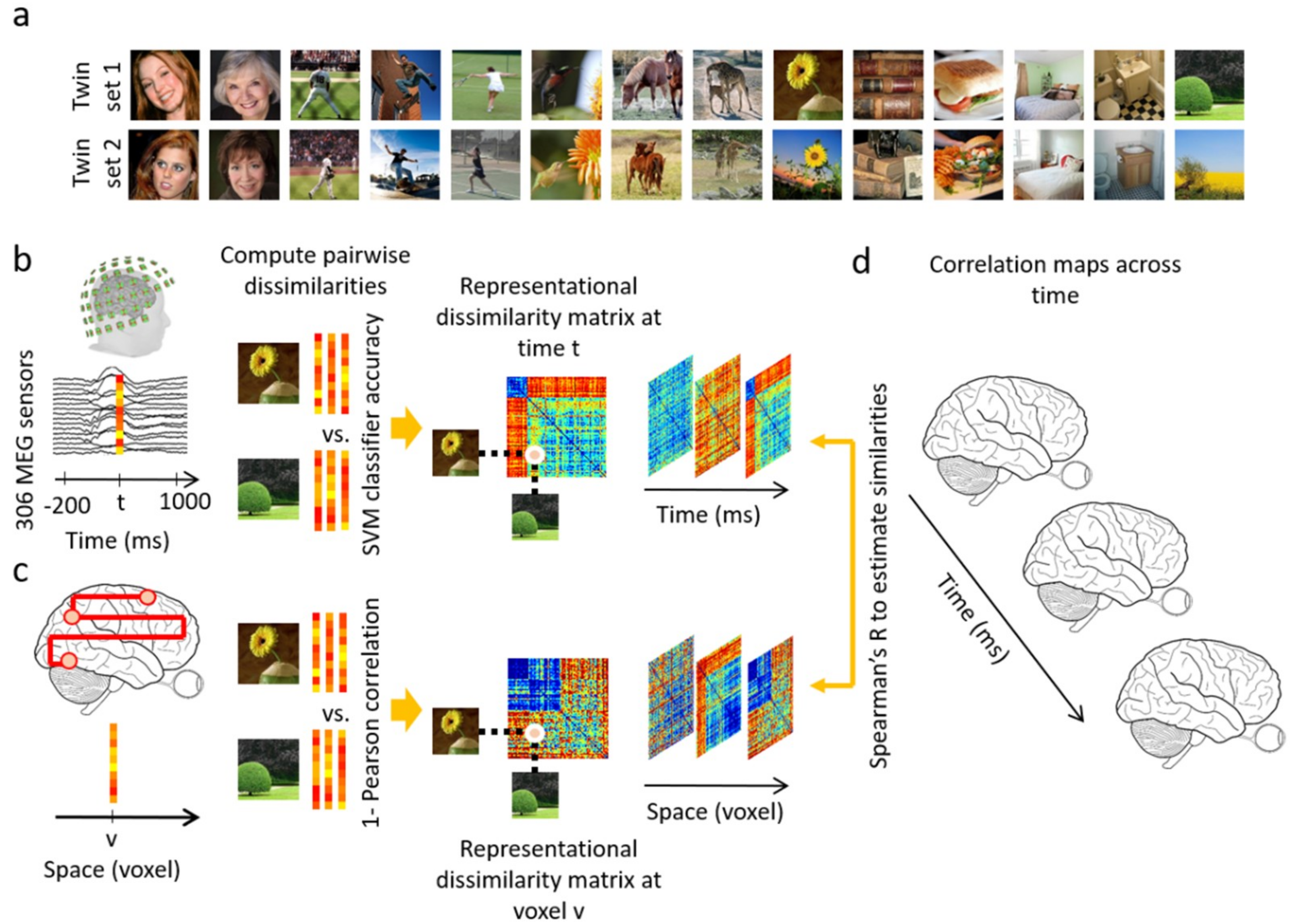
2.2. Stimulus Set
2.3. fMRI and MEG Acquisition
2.4. Data Analyses
3. Results
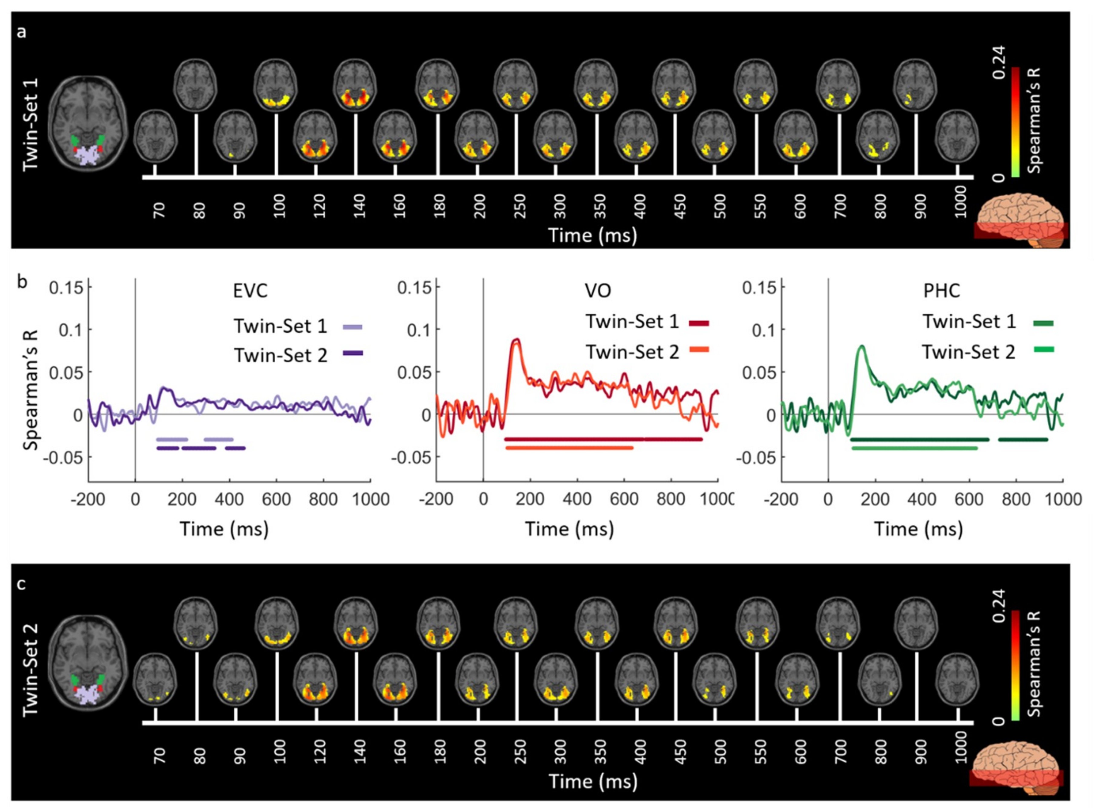
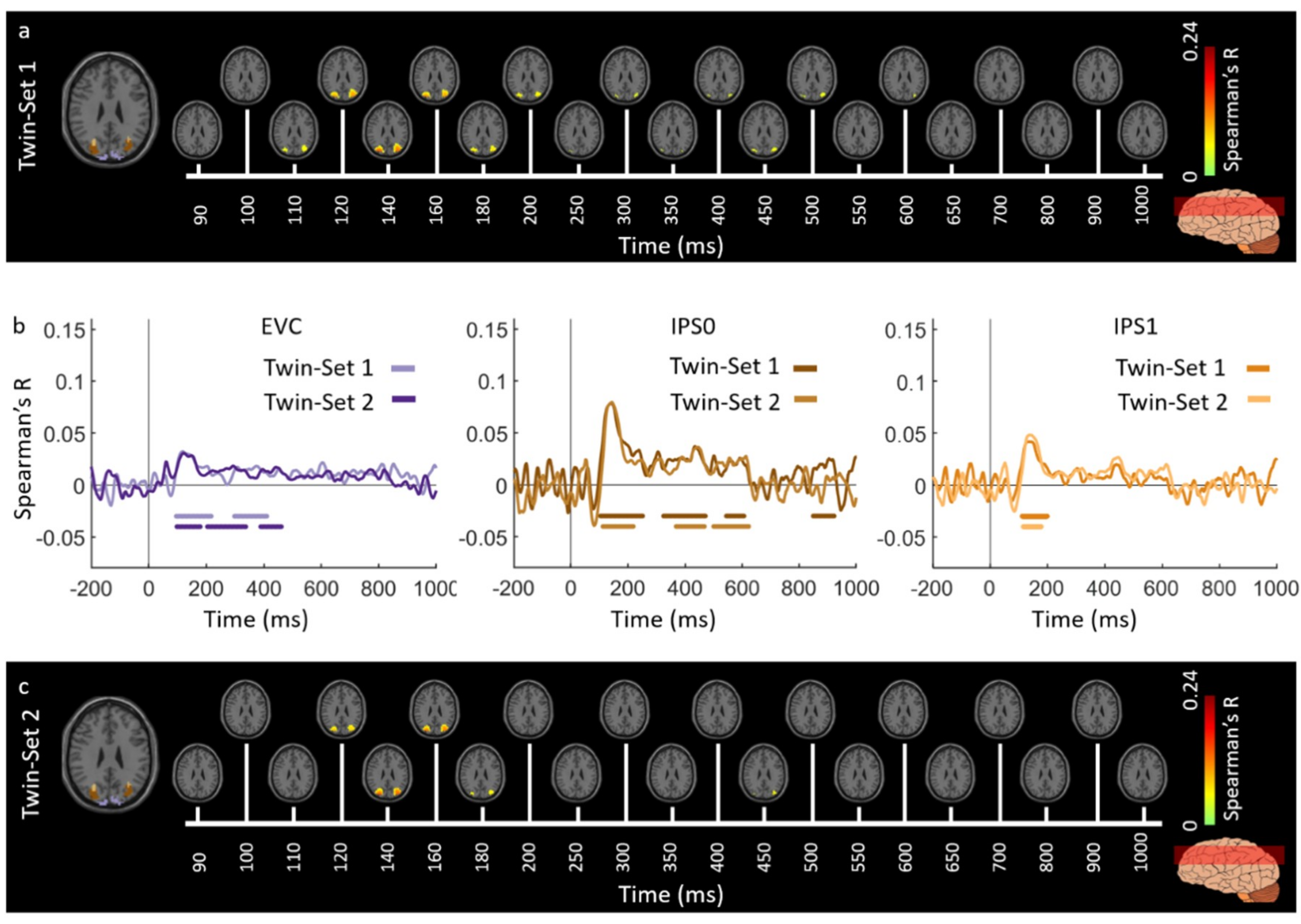
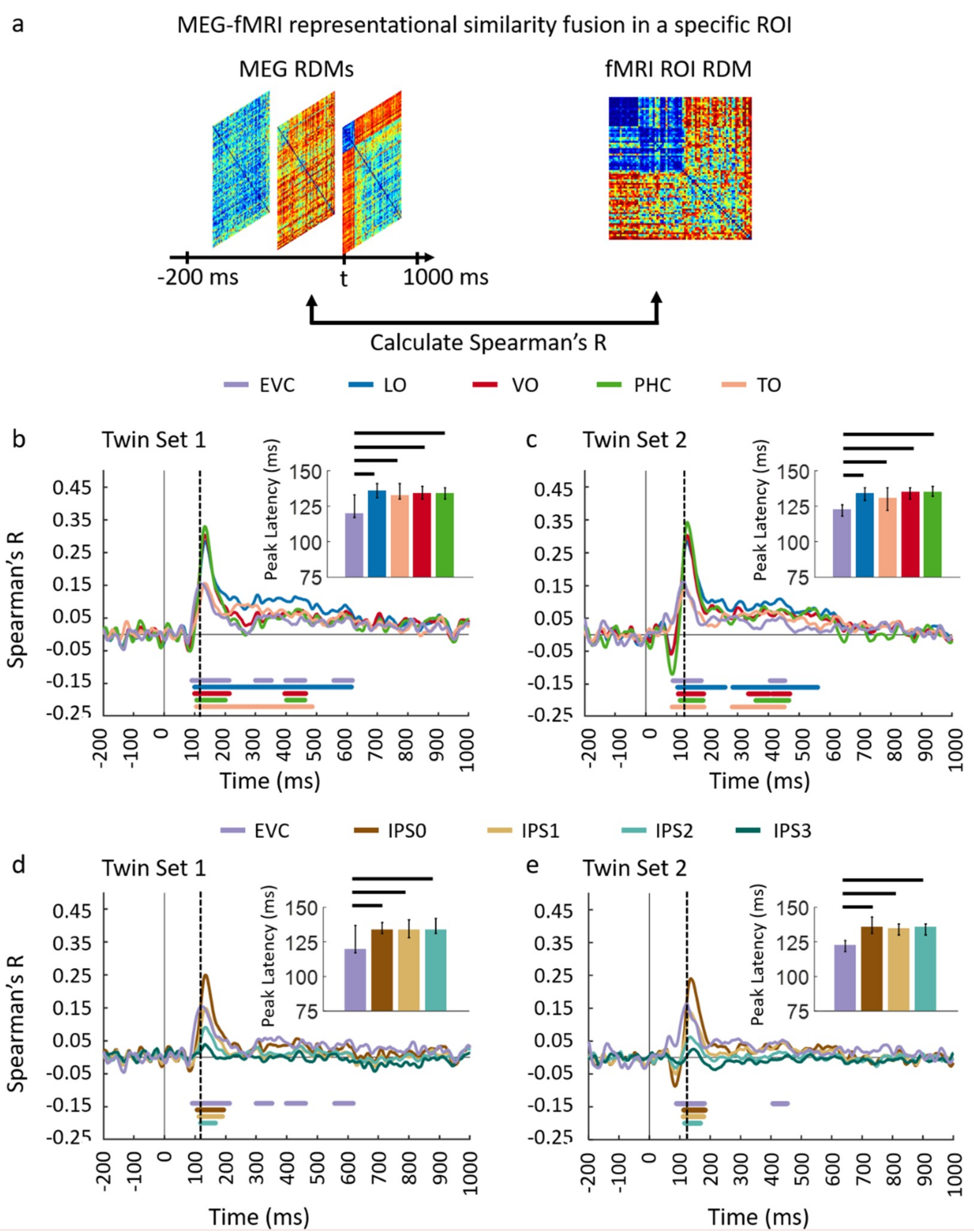
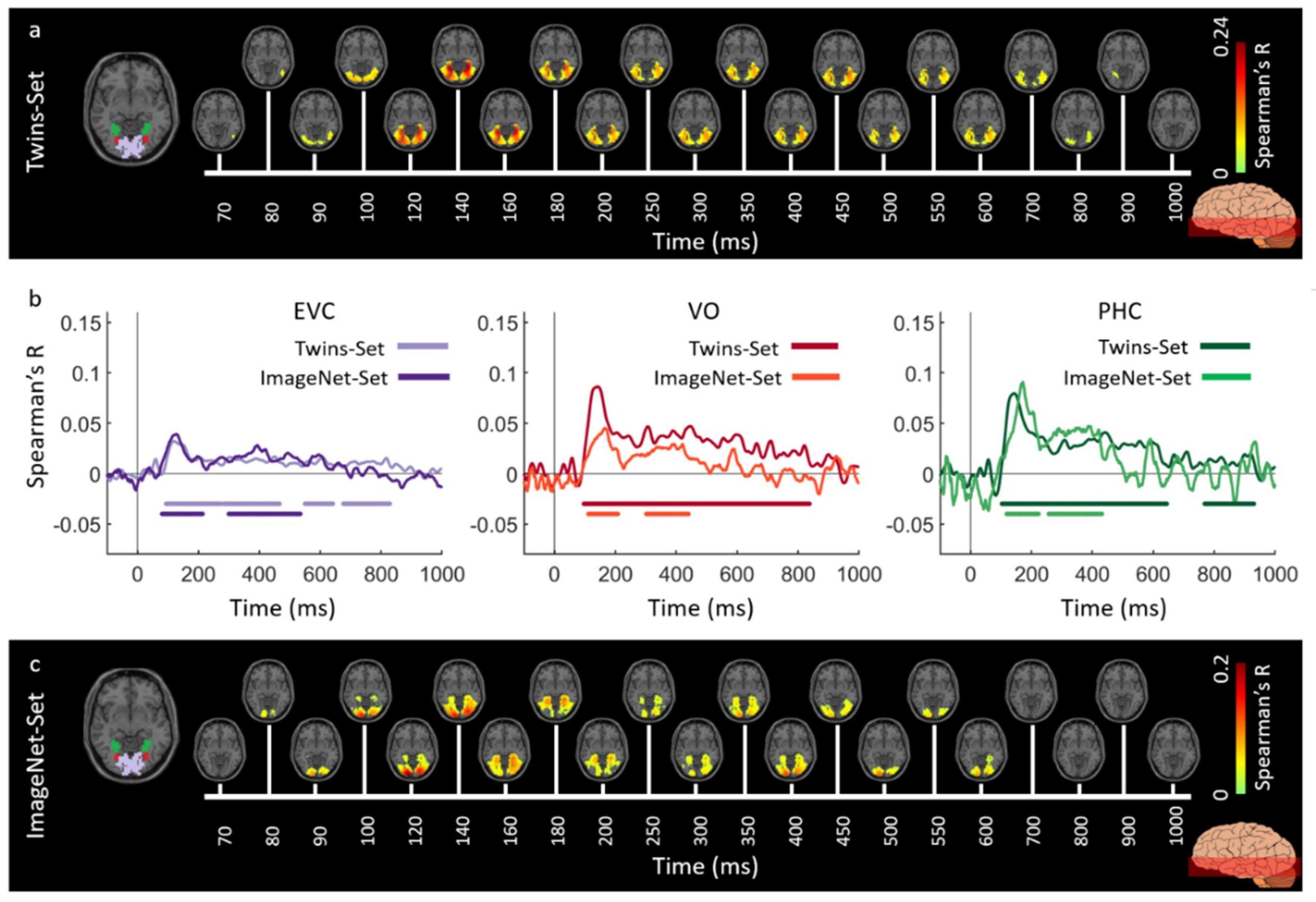
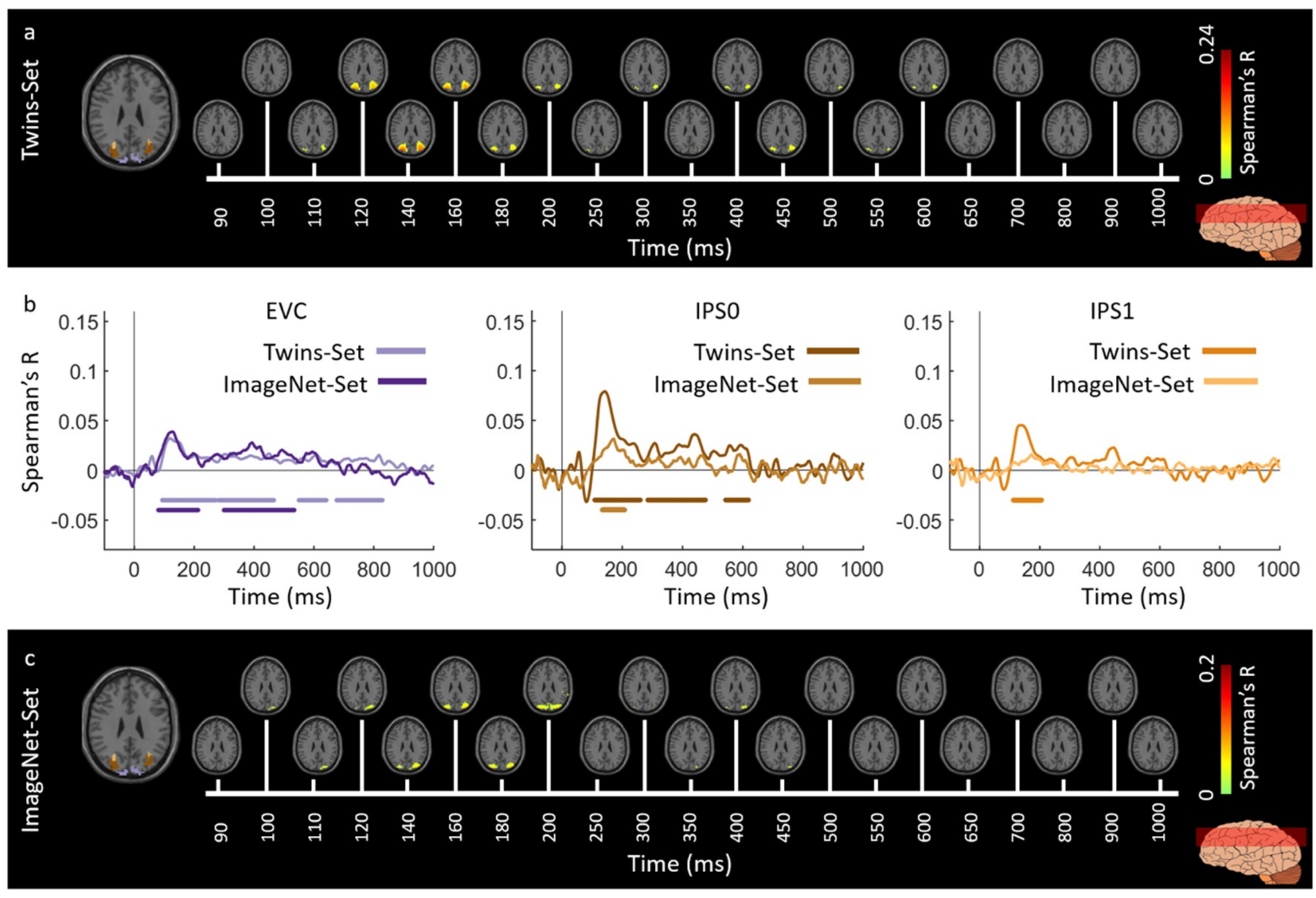
3.1. Reliability of Similarity-Based fMRI-MEG Fusion Method
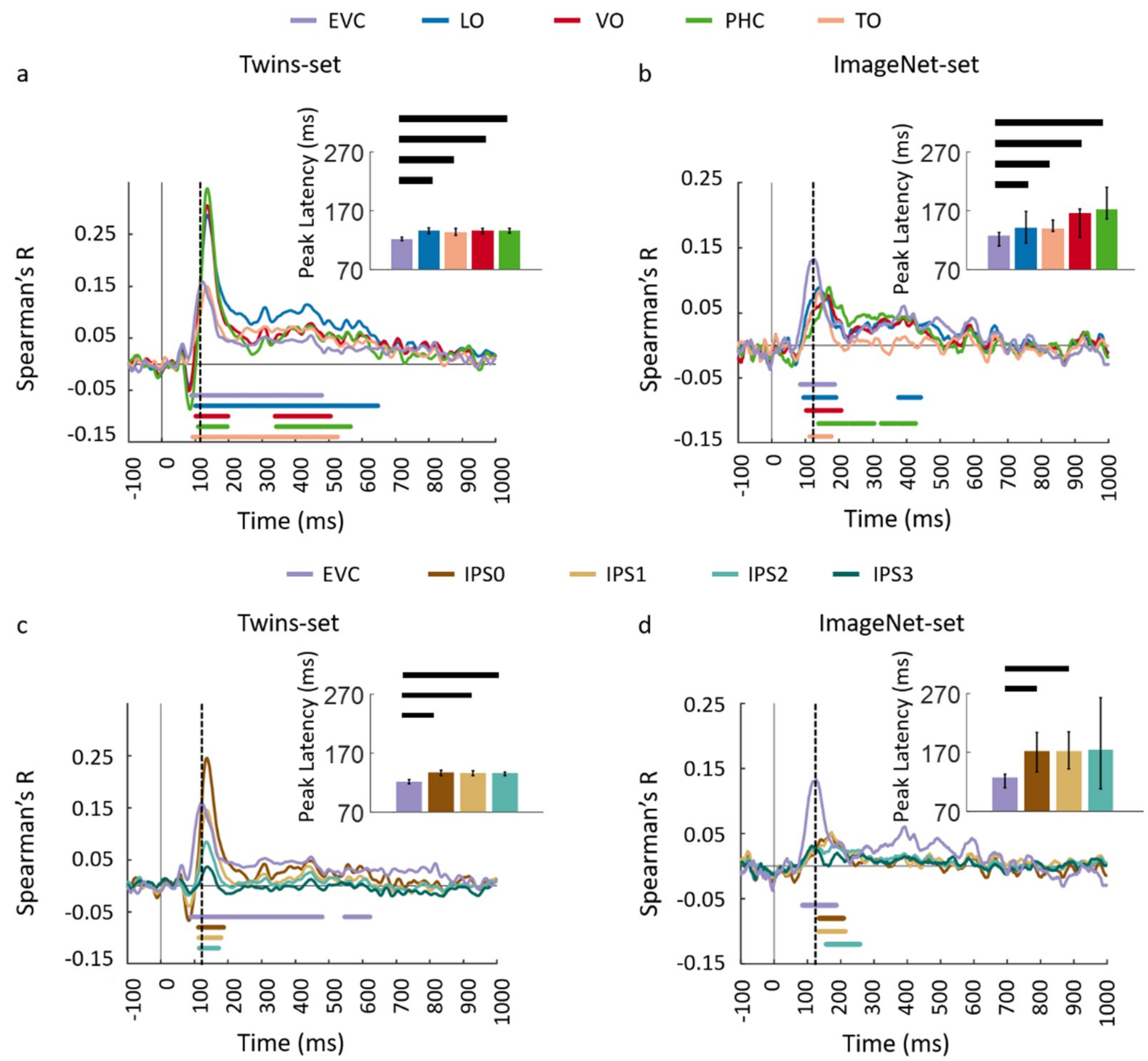
3.2. Generalizability of Similarity-Based fMRI-MEG Fusion Method
4. Discussion
Author Contributions
Funding
Acknowledgments
Conflicts of Interest
Appendix A

| Spectral Energy Level (Spatial Frequency) | ||||
|---|---|---|---|---|
| 10% | 30% | 70% | 90% | |
| t value | −0.43 | 0.87 | 0.37 | −0.37 |
| p value | 0.67 | 0.37 | 0.7 | 0.72 |
| Color Distribution | ||||||
|---|---|---|---|---|---|---|
| RGB Space | Lab Space (Brightness and Contrast) | |||||
| R | G | B | L | a | b | |
| t value | 0.65 | 0.99 | 0.71 | 0.87 | −0.80 | 0.05 |
| p value | 0.51 | 0.32 | 0.48 | 0.38 | 0.43 | 0.96 |
Appendix B
MEG Acquisition and Analysis
fMRI Acquisition and Analysis
Appendix C
Appendix D
Region-of-Interest Analysis
Appendix E
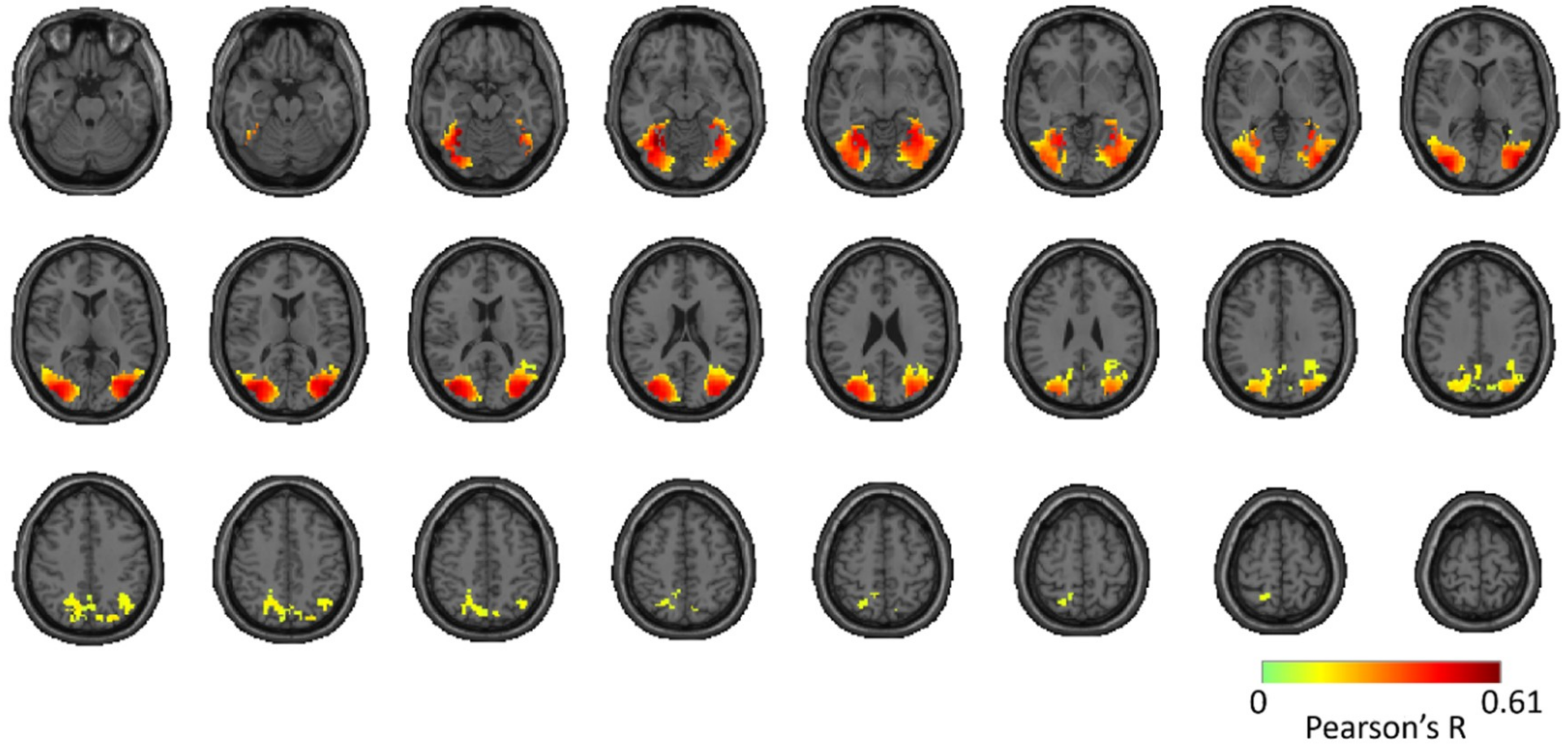
Reliability Maps
Appendix F
Statistical Testing
References
- Malach, R.; Reppas, J.B.; Benson, R.R.; Kwong, K.K.; Jiang, H.; Kennedy, W.A.; Ledden, P.J.; Brady, T.J.; Rosen, B.R.; Tootell, R.B. Object-related activity revealed by functional magnetic resonance imaging in human occipital cortex. Proc. Natl. Acad. Sci. USA 1995, 92, 8135–8139. [Google Scholar] [CrossRef] [PubMed]
- Grill-Spector, K.; Kourtzi, Z.; Kanwisher, N. The lateral occipital complex and its role in object recognition. Vis. Res. 2001, 41, 1409–1422. [Google Scholar] [CrossRef] [Green Version]
- Johnson, J.S.; Olshausen, B.A. Timecourse of neural signatures of object recognition. J. Vis. 2003, 3, 4. [Google Scholar] [CrossRef]
- Op de Beeck, H.P.; Baker, C.I. The neural basis of visual object learning. Trends Cogn. Sci. 2010, 14, 22–30. [Google Scholar] [CrossRef] [PubMed] [Green Version]
- Mullin, C.R.; Steeves, J.K.E. Consecutive TMS-fMRI Reveals an Inverse Relationship in BOLD Signal between Object and Scene Processing. J. Neurosci. 2013, 33, 19243–19249. [Google Scholar] [CrossRef] [PubMed] [Green Version]
- DiCarlo, J.J.; Zoccolan, D.; Rust, N.C. How Does the Brain Solve Visual Object Recognition? Neuron 2012, 73, 415–434. [Google Scholar] [CrossRef] [PubMed] [Green Version]
- Konkle, T.; Oliva, A. A Real-World Size Organization of Object Responses in Occipitotemporal Cortex. Neuron 2012, 74, 1114–1124. [Google Scholar] [CrossRef] [Green Version]
- Cichy, R.M.; Pantazis, D.; Oliva, A. Resolving human object recognition in space and time. Nat. Neurosci. 2014, 17, 455–462. [Google Scholar] [CrossRef] [Green Version]
- Cichy, R.M.; Pantazis, D.; Oliva, A. Similarity-Based Fusion of MEG and fMRI Reveals Spatio-Temporal Dynamics in Human Cortex During Visual Object Recognition. Cereb. Cortex 2016, 26, 3563–3579. [Google Scholar] [CrossRef] [Green Version]
- Dale, A.M.; Halgren, E. Spatiotemporal mapping of brain activity by integration of multiple imaging modalities. Curr. Opin. Neurobiol. 2001, 11, 202–208. [Google Scholar] [CrossRef]
- Debener, S.; Ullsperger, M.; Siegel, M.; Engel, A.K. Single-trial EEG–fMRI reveals the dynamics of cognitive function. Trends Cogn. Sci. 2006, 10, 558–563. [Google Scholar] [CrossRef] [PubMed] [Green Version]
- Rosa, M.J.; Daunizeau, J.; Friston, K.J. EEG-fMRI Integration: A Critical Review of Biophysical Modeling and Data Analysis Approaches. J. Integr. Neurosci. 2010, 09, 453–476. [Google Scholar] [CrossRef]
- Huster, R.J.; Debener, S.; Eichele, T.; Herrmann, C.S. Methods for Simultaneous EEG-fMRI: An Introductory Review. J. Neurosci. 2012, 32, 6053–6060. [Google Scholar] [CrossRef] [PubMed] [Green Version]
- Jorge, J.; van der Zwaag, W.; Figueiredo, P. EEG–fMRI integration for the study of human brain function. NeuroImage 2014, 102, 24–34. [Google Scholar] [CrossRef] [PubMed]
- Sui, J.; Adali, T.; Yu, Q.; Chen, J.; Calhoun, V.D. A review of multivariate methods for multimodal fusion of brain imaging data. J. Neurosci. Methods 2012, 204, 68–81. [Google Scholar] [CrossRef] [PubMed] [Green Version]
- Khaligh-Razavi, S.-M.; Cichy, R.M.; Pantazis, D.; Oliva, A. Tracking the Spatiotemporal Neural Dynamics of Real-world Object Size and Animacy in the Human Brain. J. Cogn. Neurosci. 2018, 30, 1559–1576. [Google Scholar] [CrossRef] [PubMed]
- Mohsenzadeh, Y.; Qin, S.; Cichy, R.M.; Pantazis, D. Ultra-Rapid serial visual presentation reveals dynamics of feedforward and feedback processes in the ventral visual pathway. eLife 2018, 7, 1–23. [Google Scholar] [CrossRef] [PubMed]
- Hebart, M.N.; Bankson, B.B.; Harel, A.; Baker, C.I.; Cichy, R.M. The representational dynamics of task and object processing in humans. eLife 2018, 7, 1–22. [Google Scholar] [CrossRef]
- Thorpe, S.; Fize, D.; Marlot, C. Speed of processing in the human visual system. Nature 1996, 381, 520–522. [Google Scholar] [CrossRef]
- VanRullen, R.; Thorpe, S.J. The Time Course of Visual Processing: From Early Perception to Decision-Making. J. Cogn. Neurosci. 2001, 13, 454–461. [Google Scholar] [CrossRef] [Green Version]
- Mormann, F.; Kornblith, S.; Quiroga, R.Q.; Kraskov, A.; Cerf, M.; Fried, I.; Koch, C. Latency and Selectivity of Single Neurons Indicate Hierarchical Processing in the Human Medial Temporal Lobe. J. Neurosci. 2008, 28, 8865–8872. [Google Scholar] [CrossRef] [PubMed] [Green Version]
- Liu, H.; Agam, Y.; Madsen, J.R.; Kreiman, G. Timing, Timing, Timing: Fast Decoding of Object Information from Intracranial Field Potentials in Human Visual Cortex. Neuron 2009, 62, 281–290. [Google Scholar] [CrossRef] [PubMed] [Green Version]
- Isik, L.; Meyers, E.M.; Leibo, J.Z.; Poggio, T. The dynamics of invariant object recognition in the human visual system. J. Neurophysiol. 2014, 111, 91–102. [Google Scholar] [CrossRef] [PubMed] [Green Version]
- Carlson, T.; Tovar, D.A.; Alink, A.; Kriegeskorte, N. Representational dynamics of object vision: The first 1000 ms. J. Vis. 2013, 13, 1. [Google Scholar] [CrossRef] [PubMed]
- Contini, E.W.; Wardle, S.G.; Carlson, T.A. Decoding the time-course of object recognition in the human brain: From visual features to categorical decisions. Neuropsychologia 2017, 105, 165–176. [Google Scholar] [CrossRef] [PubMed]
- Lowe, M.X.; Rajsic, J.; Ferber, S.; Walther, D.B. Discriminating scene categories from brain activity within 100 milliseconds. Cortex 2018, 106, 275–287. [Google Scholar] [CrossRef]
- Simmons, J.P.; Nelson, L.D.; Simonsohn, U. False-Positive Psychology: Undisclosed Flexibility in Data Collection and Analysis Allows Presenting Anything as Significant. Psychol. Sci. 2011, 22, 1359–1366. [Google Scholar] [CrossRef]
- Pashler, H.; Harris, C.R. Is the Replicability Crisis Overblown? Three Arguments Examined. Perspect. Psychol. Sci. 2012, 7, 531–536. [Google Scholar] [CrossRef] [Green Version]
- Bennett, C.M.; Miller, M.B. fMRI reliability: Influences of task and experimental design. Cogn. Affect. Behav. Neurosci. 2013, 13, 690–702. [Google Scholar] [CrossRef]
- Kanwisher, N.; McDermott, J.; Chun, M.M. The Fusiform Face Area: A Module in Human Extrastriate Cortex Specialized for Face Perception. J. Neurosci. 1997, 17, 4302–4311. [Google Scholar] [CrossRef] [Green Version]
- Epstein, R.; Harris, A.; Stanley, D.; Kanwisher, N. The Parahippocampal Place Area: Recognition, Navigation, or Encoding? Neuron 1999, 23, 115–125. [Google Scholar] [CrossRef]
- Epstein, R.; Kanwisher, N. A cortical representation of the local visual environment. Nature 1998, 392, 598–601. [Google Scholar] [CrossRef] [PubMed]
- Downing, P.E. A Cortical Area Selective for Visual Processing of the Human Body. Science 2001, 293, 2470–2473. [Google Scholar] [CrossRef] [PubMed] [Green Version]
- Grill-Spector, K.; Kushnir, T.; Edelman, S.; Avidan, G.; Itzchak, Y.; Malach, R. Differential Processing of Objects under Various Viewing Conditions in the Human Lateral Occipital Complex. Neuron 1999, 24, 187–203. [Google Scholar] [CrossRef] [Green Version]
- Dilks, D.D.; Julian, J.B.; Paunov, A.M.; Kanwisher, N. The Occipital Place Area Is Causally and Selectively Involved in Scene Perception. J. Neurosci. 2013, 33, 1331–1336. [Google Scholar] [CrossRef] [PubMed] [Green Version]
- Khosla, A.; Raju, A.S.; Torralba, A.; Oliva, A. Understanding and Predicting Image Memorability at a Large Scale. In Proceedings of the 2015 IEEE International Conference on Computer Vision (ICCV), Santiago, Chile, 7–13 December 2015; pp. 2390–2398. [Google Scholar]
- Torralba, A.; Oliva, A. Statistics of natural image categories. Netw. Comput. Neural Syst. 2003, 14, 391–412. [Google Scholar] [CrossRef]
- Bainbridge, W.A.; Oliva, A. A toolbox and sample object perception data for equalization of natural images. Data Brief 2015, 5, 846–851. [Google Scholar] [CrossRef] [PubMed] [Green Version]
- Park, S.; Konkle, T.; Oliva, A. Parametric Coding of the Size and Clutter of Natural Scenes in the Human Brain. Cereb. Cortex 2015, 25, 1792–1805. [Google Scholar] [CrossRef] [PubMed]
- Deng, J.; Dong, W.; Socher, R.; Li, L.-J.; Li, K.; Fei-Fei, L. ImageNet: A Large-Scale Hierarchical Image Database. In Proceedings of the 2009 IEEE Conference on Computer Vision and Pattern Recognition, Miami, FL, USA, 20–25 June 2009. [Google Scholar]
- Kriegeskorte, N. Representational similarity analysis—Connecting the branches of systems neuroscience. Front. Syst. Neurosci. 2008, 2, 4. [Google Scholar] [CrossRef]
- Kriegeskorte, N.; Kievit, R.A. Representational geometry: Integrating cognition, computation, and the brain. Trends Cogn. Sci. 2013, 17, 401–412. [Google Scholar] [CrossRef]
- John, L.K.; Loewenstein, G.; Prelec, D. Measuring the Prevalence of Questionable Research Practices With Incentives for Truth Telling. Psychol. Sci. 2012, 23, 524–532. [Google Scholar] [CrossRef] [PubMed]
- Maxwell, S.E.; Lau, M.Y.; Howard, G.S. Is psychology suffering from a replication crisis? What does “failure to replicate” really mean? Am. Psychol. 2015, 70, 487–498. [Google Scholar] [CrossRef] [PubMed]
- Munafò, M.R.; Nosek, B.A.; Bishop, D.V.M.; Button, K.S.; Chambers, C.D.; Percie du Sert, N.; Simonsohn, U.; Wagenmakers, E.-J.; Ware, J.J.; Ioannidis, J.P.A. A manifesto for reproducible science. Nat. Hum. Behav. 2017, 1, 0021. [Google Scholar] [CrossRef] [Green Version]
- Haynes, J.-D.; Rees, G. Decoding mental states from brain activity in humans. Nat. Rev. Neurosci. 2006, 7, 523–534. [Google Scholar] [CrossRef]
- Grill-Spector, K.; Malach, R. THE HUMAN VISUAL CORTEX. Annu. Rev. Neurosci. 2004, 27, 649–677. [Google Scholar] [CrossRef] [PubMed]
- Op de Beeck, H.P.; Haushofer, J.; Kanwisher, N.G. Interpreting fMRI data: Maps, modules and dimensions. Nat. Rev. Neurosci. 2008, 9, 123–135. [Google Scholar] [CrossRef] [PubMed]
- Amano, K. Estimation of the Timing of Human Visual Perception from Magnetoencephalography. J. Neurosci. 2006, 26, 3981–3991. [Google Scholar] [CrossRef] [PubMed] [Green Version]
- Ioannidis, J.P.A. Why Most Published Research Findings Are False. PLoS Med. 2005, 2, 6. [Google Scholar] [CrossRef] [PubMed]
- Button, K.S.; Ioannidis, J.P.A.; Mokrysz, C.; Nosek, B.A.; Flint, J.; Robinson, E.S.J.; Munafò, M.R. Power failure: Why small sample size undermines the reliability of neuroscience. Nat. Rev. Neurosci. 2013, 14, 365–376. [Google Scholar] [CrossRef] [PubMed]
- Riesenhuber, M.; Poggio, T. Neural mechanisms of object recognition. Curr. Opin. Neurobiol. 2002, 12, 162–168. [Google Scholar] [CrossRef] [Green Version]
- Serre, T.; Oliva, A.; Poggio, T. A feedforward architecture accounts for rapid categorization. Proc. Natl. Acad. Sci. USA 2007, 104, 6424–6429. [Google Scholar] [CrossRef] [PubMed] [Green Version]
- Caceres, A.; Hall, D.L.; Zelaya, F.O.; Williams, S.C.R.; Mehta, M.A. Measuring fMRI reliability with the intra-class correlation coefficient. NeuroImage 2009, 45, 758–768. [Google Scholar] [CrossRef] [PubMed]
- Miller, M.B.; Van Horn, J.D. Individual variability in brain activations associated with episodic retrieval: A role for large-scale databases. Int. J. Psychophysiol. 2007, 63, 205–213. [Google Scholar] [CrossRef] [PubMed]
- Taulu, S.; Kajola, M.; Simola, J. Suppression of Interference and Artifacts by the Signal Space Separation Method. Brain Topogr. 2003, 16, 269–275. [Google Scholar] [CrossRef]
- Taulu, S.; Simola, J. Spatiotemporal signal space separation method for rejecting nearby interference in MEG measurements. Phys. Med. Biol. 2006, 51, 1759–1768. [Google Scholar] [CrossRef] [PubMed]
- Tadel, F.; Baillet, S.; Mosher, J.C.; Pantazis, D.; Leahy, R.M. Brainstorm: A User-Friendly Application for MEG/EEG Analysis. Comput. Intell. Neurosci. 2011, 2011, 1–13. [Google Scholar] [CrossRef] [PubMed] [Green Version]
- Kriegeskorte, N.; Goebel, R.; Bandettini, P. Information-based functional brain mapping. Proc. Natl. Acad. Sci. USA 2006, 103, 3863–3868. [Google Scholar] [CrossRef] [Green Version]
- Haynes, J.-D.; Sakai, K.; Rees, G.; Gilbert, S.; Frith, C.; Passingham, R.E. Reading Hidden Intentions in the Human Brain. Curr. Biol. 2007, 17, 323–328. [Google Scholar] [CrossRef] [Green Version]
- Wang, L.; Mruczek, R.E.B.; Arcaro, M.J.; Kastner, S. Probabilistic Maps of Visual Topography in Human Cortex. Cereb. Cortex 2015, 25, 3911–3931. [Google Scholar] [CrossRef]
- Maris, E.; Oostenveld, R. Nonparametric statistical testing of EEG- and MEG-data. J. Neurosci. Methods 2007, 164, 177–190. [Google Scholar] [CrossRef]
- Pantazis, D.; Nichols, T.E.; Baillet, S.; Leahy, R.M. A comparison of random field theory and permutation methods for the statistical analysis of MEG data. NeuroImage 2005, 25, 383–394. [Google Scholar] [CrossRef] [PubMed]


| Region of Interest | Twin-Set 1 | Twin-Set 2 | ||
|---|---|---|---|---|
| Peak latency (ms) | Onset latency (ms) | Peak latency (ms) | Onset latency (ms) | |
| EVC | 120 (117–137) | 92 (85–99) | 123 (118–126) | 90 (51–94) |
| Dorsal regions | ||||
| IPS0 | 134 (131–139) | 107 (97–116) | 136 (131–143) | 113 (107–118) |
| IPS1 | 134 (128–141) | 113 (102–123) | 135 (130–138) | 111 (105–116) |
| IPS2 | 134 (131–142) | 118 (95–156) | 136 (130–138) | 116 (107–126) |
| Ventral regions | ||||
| LO | 136 (131–141) | 101 (95–107) | 134 (129–138) | 105 (100–108) |
| VO | 134 (130–139) | 100 (95–105) | 135 (130–138) | 104 (99–111) |
| TO | 133 (130–141) | 104 (92–111) | 131 (122–138) | 85 (73–101) |
| PHC | 134 (130–138) | 106 (99–113) | 135 (132–139) | 112 (107–116) |
| Region of Interest | Twins-Set | ImageNet-Set | ||
|---|---|---|---|---|
| Peak latency (ms) | Onset latency (ms) | Peak latency (ms) | Onset latency (ms) | |
| EVC | 122 (119–125) | 89 (56–95) | 127 (110–133) | 84 (71–91) |
| Dorsal regions | ||||
| IPS0 | 137 (131–141) | 111 (102–117) | 172 (137–204) | 133 (99–156) |
| IPS1 | 136 (132–140) | 111 (103–119) | 172 (142–205) | 137 (99–158) |
| IPS2 | 136 (132–138) | 112 (100–119) | 174 (108–263) | 103 (90–186) |
| Ventral regions | ||||
| LO | 136 (131–141) | 102 (97–107) | 141 (115–169) | 96 (87–118) |
| VO | 136 (131–139) | 102 (95–109) | 166 (125–173) | 103 (95–125) |
| TO | 134 (128–140) | 90 (77–100) | 139 (135–154) | 115 (95–126) |
| PHC | 136 (132–139) | 109 (102–115) | 172 (156–210) | 121 (99–159) |
© 2019 by the authors. Licensee MDPI, Basel, Switzerland. This article is an open access article distributed under the terms and conditions of the Creative Commons Attribution (CC BY) license (http://creativecommons.org/licenses/by/4.0/).
Share and Cite
Mohsenzadeh, Y.; Mullin, C.; Lahner, B.; Cichy, R.M.; Oliva, A. Reliability and Generalizability of Similarity-Based Fusion of MEG and fMRI Data in Human Ventral and Dorsal Visual Streams. Vision 2019, 3, 8. https://doi.org/10.3390/vision3010008
Mohsenzadeh Y, Mullin C, Lahner B, Cichy RM, Oliva A. Reliability and Generalizability of Similarity-Based Fusion of MEG and fMRI Data in Human Ventral and Dorsal Visual Streams. Vision. 2019; 3(1):8. https://doi.org/10.3390/vision3010008
Chicago/Turabian StyleMohsenzadeh, Yalda, Caitlin Mullin, Benjamin Lahner, Radoslaw Martin Cichy, and Aude Oliva. 2019. "Reliability and Generalizability of Similarity-Based Fusion of MEG and fMRI Data in Human Ventral and Dorsal Visual Streams" Vision 3, no. 1: 8. https://doi.org/10.3390/vision3010008