Article

Modeling, Simulation and Control of the Walking of Biped Robotic Devices, Part II: Rectilinear Walking

Control and Computer Engineering Department, Politecnico di Torino, Corso Duca degli Abruzzi 24, 10124 Torino, Italy
*
Author to whom correspondence should be addressed.
These authors contributed equally to this work.
Inventions 2016, 1(1), 7; https://doi.org/10.3390/inventions1010007
Submission received: 24 November 2015 / Revised: 2 March 2016 / Accepted: 7 March 2016 / Published: 22 March 2016

Abstract

:
This is the second part of a three-part paper. It extends to the free walking results of a previous work on postural equilibrium of a lower limb exoskeleton for rehabilitation exercises. A classical approach has been adopted to design gait (zero moment point (ZMP), linearized inverted pendulum theory, inverse kinematics obtained through the pseudo-inverse of Jacobian matrices). While several ideas exploited here can be found in other papers of the literature, e.g., whole-body coordination, our contribution is the simplicity of the whole control approach that originates logically from a common root. (1) The approximation of the unilateral foot/feet-ground contacts with non-holonomic constraints leads naturally to a modeling and control design that implements a two-phase switching system. The approach is facilitated by Kane’s method and tools as described in Part I. (2) The Jacobian matrix is used to transfer from the Cartesian to the joint space a greater number of variables for redundancy than the degrees of freedom (DOF). We call it the extended Jacobian matrix. Redundancy and the prioritization of postural tasks is approached with weighted least squares. The singularity of the kinematics when knees are fully extended is solved very simply by fake knee joint velocities. (3) Compliance with the contact and accommodation of the swing foot on an uneven ground, when switching from single to double stance, and the transfer of weight from one foot to the other in double stance are approached by exploiting force/torque expressions returned from the constraints. (4) In the center of gravity (COG)/ZMP loop for equilibrium, an extended estimator, based on the linearized inverted pendulum, is adopted to cope with external force disturbances and unmodeled dynamics. Part II treats rectilinear walking, while Part III discusses turning while walking.

1. Introduction

This paper deals with the control of a biped robotic device during walking, specifically an exoskeleton haptic device for use in lower limb rehabilitation or an autonomous biped robot. This research was originally motivated by the design of an exoskeleton for lower limb rehabilitation (see [1]). However, that device was not intended for walking, but only to operate in a fixed position. The possible exercises, designed for the early stages of rehabilitation, are preparatory to actual gait and account for motions in the sagittal plane, as in sit-to-stand exercises, or in the frontal plane by simulating walking, as in a step machine. The approach proposed is based on a closed loop position control designed to maintain or recover postural equilibrium, contemporaneously offering patient compliance through a mechanical admittance control. Admittance control offers a dynamic mapping from force to motion, where force information from the patient is obtained from bioelectrical signals, e.g., electromyographic (EMG) signals, measured on proper pairs of antagonistic muscles in the patient’s legs. Briefly, the control system is based on two hierarchical feedback loops:
  • An inner one, embedding admittance control in a position loop, which closes a feedback from exoskeleton joint positions and velocities. This is solved by the linearization of the model of the exoskeleton and patient joined together. A two degrees of freedom approach is adopted using multivariable robust control theory. The exoskeleton is compliant with the patient’s efforts in the neighborhood of given joint angle reference positions, and this is according to an imposed admittance driven by the patient’s EMG signals.
  • An outer control loop, closing a feedback from measurements performed on the feet-sole center of pressure (CoP) (i.e., zero moment point (ZMP)), corrects the joint angle reference positions in the inner loop, in order to maintain postural equilibrium.
The resulting control of the joint angles allows a reference position to be tracked in time, contemporaneously offering compliance with the patient, according to the assigned mechanical admittance. Hence, the exoskeleton joints are driven by two targets, often competing at the early stage of the rehabilitation therapy and hopefully cooperating (this is the objective of the rehabilitation training) at the conclusion of the same therapy, i.e., forces (measured by EMG signals), which are to be complied with, and position, which assure posture. The degree of the tracking of each of these two targets is governed by the imposed admittance, chosen by the therapist at the different stages of rehabilitation. A high admittance means that the exoskeleton is highly compliant with the efforts of the patient; low admittance strongly constrains the patient and answers primarily to the postural equilibrium requirements of the outer control loop. In both cases, the outer control loop sustains the patient against gravity and helps the patient to maintain equilibrium during her/his exercises, by correcting the position references, tracked in the inner control loop. Postural equilibrium is also enhanced, when necessary, by dynamically reducing the admittance of the response, when the boundaries of equilibrium are reached (thus inhibiting a patient’s erroneous posture).
Although being efficient for controlling exercises during the early stages of rehabilitation, this system does not offer any solution to the problem of controlling a biped robotic device during walking. The aim of this work is to extend those results, overcoming well-known criticalities with a simple and efficient control during walking, while still maintaining the postural equilibrium enhancement and compliance with the patient. However, the approach can be adopted for the control of an autonomous biped robot, as well.

1.1. State of the Art of Bipedal Gait Control

To date, there have been a number of three-dimensional bipedal walking robots developed, such as the Honda P2, P3 and ASIMO [2,3], Sony QRIO [4], University of Munich’s Johnnie [5], Kawada/AIST HRP-1S [6], HUBO by Oh, Park et al. [7] and, more recently, the line of research related to whole-body-coordination [8,9,10]. The approaches proposed in the literature to obtain a dynamically-stable gait can be classified as model based or model-less. The former can be further divided into four groups, according to whether they:
  • exploit a detailed model description to maintain equilibrium [11];
  • or rely on a simplified linearized inverted pendulum and zero moment point theory [12];
  • track a precomputed trajectory [13];
  • or are trajectory free [7].
As a separate group, the model-less approaches belong to the “neural-oscillatory control” category [14,15].
Among the model-based approaches, those called “controls by forward dynamics” [16] exploit a complete knowledge of robot dynamics and are implemented in the framework of a mechanical system, which is subject to unilateral constraints. These are known as hybrid complementarity dynamical systems [17] and are mostly used to study gait theoretically and to improve the understanding of the neurological aspects of human walking [18].
The practical applications, mentioned at the beginning of this section, with the exception of QRIO, which in the literature has been described as controlled by “neural-oscillators”, all use variants (either with precomputed trajectories or trajectory free) of the linearized inverted pendulum model and ZMP theory.

1.2. Gait Control

The approach proposed in this paper belongs to this latter ZMP-based family, with a precomputed trajectory. The contribution, with respect to other works of this family, is the systematic nature with which a hybrid switching control has been proposed. It covers both phases of the single and double stance of gait, solving a series of problems ranging from the selection of dependent and independent joints for the control, the compliance with the swing foot and the ground, as well as compliance with the patient, when the approach is adopted for an exoskeleton, and the singularity of the kinematics.
In order to control gait, the following technical problems have to be solved:
  • Modeling a multi-body dynamical system switching periodically between the two phases of gait: single and double stance. The dynamical behavior of the multi-body system driven by joint torques and ground reaction forces/torques is given by a system of second order non-linear differential equations, referred to as hybrid complementarity dynamical systems (see, for example, [19] Chapter 16, Section 3). This mechanical system is subject to changing unilateral constraints represented by the contact of the soles of the supporting foot/feet with the ground. The resulting reactions forces/torques are important for balancing the weight and postural control, as they define the ZMP, i.e., the CoP under the soles of the feet, which is the primary measure and objective of postural equilibrium.
  • Implementing gait so that nominal (open loop) trajectories of the projection of the center of gravity (COG) on the ground (and consequently, trajectories of the joint angles) satisfy, at each instant of time, precise ZMP constraints to maintain equilibrium during a dynamic walking. This requires a certain degree of motion anticipation.
  • Designing a switching feedback control to offer acceptable gait trajectories under uncertainty. This means managing compliance with the swing foot when entering in double stance and for transferring weight load.
  • Transferring reference trajectories (defined in terms of positions, velocities, constraint reaction forces and torques) from the Cartesian space to the joint space for closed loop motion control. This involves inverse kinematics in a highly non-linear dynamical environment, in the presence of singularities.
The first problem (Point 1) is approached here by approximating the system in the different phases as being subject to different non-holonomic constraints. Kane’s method [20] and tools, as described in Part I, are employed for all relevant mathematics. This helps to select independent and dependent joint variables for the control, to obtain both lower order kinematics and dynamics and explicit expressions of force/torque reactions at the constraints. Such an assumption may be acceptable as unilateral ground constraints do not come into play in normal conditions; however, orthogonal and tangential forces under the feet are continuously monitored for detachment or slipping to assure the control is consistent.
For the second problem (Point 2), nominal COG trajectories during the different phases of the stride are based on the linearized inverted pendulum theory, interleaving a periodic behavior, as discussed in a recent work of Choi [9], with transients computed using early works on preview control, e.g., [13] or [21].
For the third problem (Point 3), a multivariable position feedback has been designed, switching redundant joints, during the over-actuated double stance, to control reaction force/torques at the feet.
The control of COG/ZMP, critical for equilibrium, has been approached improving an idea of Choi with the aim to cope with model uncertainty, by introducing an extended estimator and state feedback.
For the fourth problem (Point 4), techniques based on the Jacobian matrix are adopted to perform the inverse kinematics, by constraining the trajectory of points and attitudes of bodies of the multi-chain on the Cartesian space in number greater than the DOF of the mode. This is done specifically by adding knee references. Redundancy in the constraints to overcome Jacobian singularity problems and modeling approximations, which is common in the literature (see [22]), can exploit in the gait fake knee joint velocities.
The biped robot and its mechanical model are described in Part I. Part II, which approaches rectilinear walking, is organized as follows: In Section 2, the general scheme of equilibrium and postural control is presented; Section 3 approaches the force control for compliance of the swing foot and load transfer; simulation of an autonomous walk of the model of an exoskeleton, which is being developed, is presented in Section 4, and Section 5 concludes the paper, with considerations of the patient’s interactions and open issues. The extension to walking while turning is discussed in Part III.

2. Controlling Gait

In Part I, the model of the biped device and a stride in the gait, with their phases and major events, was described. Refer to that part for the definition of the variables and the DOF involved in the control implemented here.

2.1. Equilibrium, Posture and Preview Signals

The approach to offer equilibrium during gait to a biped by the linearized inverted pendulum theory is well known, as well as the use of Jacobians to perform inverse kinematics.
An example of controlling the behavior of COG and ZMP embedded in a postural motion is given in [9]. Approaches of whole-body coordination solve equilibrium and postural tasks hierarchically [8,10].
Here, the linearized inverted pendulum theory and the use of Jacobians to perform inverse kinematics are exploited to control in closed loop the whole set of Cartesian variables (i.e., COG/ZMP, trunk attitude, swing foot coordinates, feet angles around y), which are necessary to uniquely determine equilibrium and posture during gait. Knee joints have been added for redundancy, using fake references, and weighted least squares are adopted for prioritization.
Note that this approach results in the design of a multivariable (switching) control, where position feedback of the independent joints is identical during both phases of the gait, while a force feedback substitutes the position control of the swing foot at the transition from single stance. It offers compliance for adaptation to an uneven ground at contact and subsequently for load transfer from the supporting foot to the other in double stance.
A detailed analysis of the reference signals (position and velocity) of the Cartesian variables involved in the equilibrium and postural tasks is given below. The figures refer to the example to be presented in Section 4. The generation of these reference trajectories is done by a preview-reference-generation module. These signals are as simple as possible, based on a few parameters, as they are synthesized in real time and, in the case of an exoskeleton, morphed adaptively from nominal trajectories, so as to be synchronous with the time events of the stride and consistent with the length of the step of the patient.
COGxy: The vectors of the reference trajectories (position and velocity) C O G x y p r e v i e w , C O ˙ G x y r e f of the x and y Cartesian coordinates of the COG have to anticipate the ZMP motion, to maintain equilibrium during gait. They are generated linking together transient behaviors using linear quadratic (LQ) optimal control with a short look-ahead horizon. For discrete time, over a short horizon, the solution can be given in a closed form to be computed in real time (see [13]), with a periodic behavior, synthesized from a set of a few parameters, as shown in [9]. The parameters are the following: Tstep is the time period of one step (2Tstep is the stride period); td, the duration of the double stance; A is half the distance between the two feet in the frontal plane; and step is the length of advancement during one step.
Figure 1 shows the preview signals of a few strides. They are generated by linking two transients from/to the center of balance and still position to a periodic behavior. The parameters of the stride are: Tstep = 0.9 s, td = 0.18 s, A = 0.17 m and step = 0.5 m.
COGz: C O G z r e f represents the desired position of the z (vertical) coordinate of the COG; for simplicity, a constant value can be chosen: C O G z r e f = c z according to the classical six determinants theory [23]; or an inverted pendulum walk can be imposed following more recent research results based on human energy consumption [24,25,26]. A constant value is assumed in the next example.
θhat: The two-dimensional vector θ h a t r e f indicates the desired average attitude of the trunk around the x and y axes (around the z axis, it has already been imposed by a non-holonomic constraint of rectilinear walking), assuming zero the angular velocities: θ x h a t r e f = 0 , θ y h a t r e f = θ 0 (the trunk slightly leaning forward).
θ y f e e t : The angle with respect to the y axis θ y f e e t r e f of both feet is assigned. It is based on three parameters: the interval of time t 1 o f f between the events of H e e l 1 o f f and H e e l 2 s t r i k e (see Figure 3 in [27]) and the maximum and minimum values θ m a x and θ m i n ; its trajectory is built by linking segments of the half period of cosine functions on an interval of t 1 o f f + T s t e p + t d . In the example of Figure 2, the parameters assume the values of 0.18 s, +25° and −10°.
Swing foot : The three-dimensional vector x s w i n g F o o t r e f and its velocity indicate the reference trajectories, for x, y and z of the lowest point of the sole of the swing foot foot2, which moves from toe2 to heel2 during the single stance period. These trajectories are synthesized in real time adopting simple functions (as before, linking segments of the half period of cosine functions) based on three parameters: step, the single stance period (i.e., Tsteptd) and the maximum height reached by the swing foot hz.
Figure 3 shows the progression of the swing foot on x and z; y is maintained constant.

2.2. The Jacobian Matrices

The Jacobian matrices of the velocities of the previous variable with respect to the independent joint velocities are indicated as:
J C O G x y s , J C O G x y d , J C O G z s , J C O G z d , which refer to the two horizontal coordinates (x, y) and the vertical coordinate (z) of the COG;
J h a t s , J h a t d to the attitude of the trunk, around the x and y axes;
J θ y f e e t s , J θ y f e e t d to the rotation around y of the feet in single and double stance (for Foot 1 it is a row of zeros with a one in the column corresponding to θ y f o o t 1 );
J s w i n g F o o t s to the three Cartesian coordinates of the swinging foot in single stance only.
All of the above Jacobians can be computed in real time from the joint angle measurements, from the assumed kinematics and weight distribution. In Kane’s method, these Jacobian expressions are explicitly given by the vectors of partial velocities in a particularly efficient form.
Define the two square matrices (10 × 10 and 7 × 7, respectively) Js and Jd, built from the above defined Jacobians for the single and double stance:
J s = J C O G x y s J C O G z s J h a t s J θ y f e e t s J s w i n g F o o t s , J d = J C O G x y d J C O G z d J h a t d J θ y f e e t d
These matrices link velocities in the Cartesian space, where the trajectories are defined, to the (independent) joint space, by the following expression:
V s J s · θ ˙ s , V d J d · θ ˙ d
where Vs, Vd are the Cartesian reference or preview velocities, given by the following expressions in single and double stance, respectively:
V s = [ C O ˙ G x y p r e v i e w T , C O ˙ G z r e f , θ ˙ h a t r e f T , θ ˙ y f e e t r e f T , x ˙ s w i n g F o o t r e f T ] T V d = [ C O ˙ G x y p r e v i e w T , C O ˙ G z r e f , θ ˙ h a t r e f T , θ ˙ y f e e t r e f T ] T
and θ ˙ s , θ ˙ d are the vectors of independent motion variables, as defined in (17) and (20) of the first part of this paper. The above Jacobian matrices become singular during gait, in particular when the legs are fully extended and the knee angles reach their maximum value. Hence, they cannot be used directly to control the Cartesian variables.

The Extended Jacobian

In order to overcome the singularities of the Jacobian, the set of imposed references is extended by adding to the vector of Cartesian velocities (on the left-hand side of the above expressions Equation (2) the velocities of the knee joint angles of the right and left legs θ ˙ k n e e 1 , θ ˙ k n e e 2 , and by properly assigning reference values as if they were given. It is to be noted that knee joint angles are independent joint variables, which are to be controlled, and are also present on the right-hand side. Hence, the following equations hold:
λ θ ˙ k n e e 1 r e f θ ˙ k n e e 2 r e f = λ · I s θ ˙ s , λ θ ˙ k n e e 1 r e f θ ˙ k n e e 2 r e f = λ · I d θ ˙ d
where Is and Id are two row matrices of all zeroes with only two elements equal to one in the appropriate column positions corresponding to the knee angles velocities in the vectors of the independent joint motion variables θ ˙ , and λ is a suitable weighting factor. Note that θ ˙ k n e e 1 or θ ˙ k n e e 2 , or both, can be added to the constraints, according to the specific control needs. The above defined Jacobian matrices Equation (1) are in this way extended to include the additional constraints, as in the following expressions:
J e x t s = J C O G x y s J C O G z s J h a t s J θ y f e e t s J s w i n g F o o t s λ · I s , J e x t d = J C O G x y d J C O G z d J h a t d J θ y f e e t d λ · I d
and are called here extended Jacobians. This is similar to Jaux and the handling of joint angle constraints in [22], with the advantage, in the gait, that the nominal periodical joint speeds of the knees that act as fake references can be exploited. This prevents singularities, and the inverse relationship from Cartesian space to joint space can now be computed (approximately) for any joint condition, by resorting to the pseudo-inverse solution, through least squares. Specifically, by adopting weighted least squares, it is possible to reduce the role of the (only approximately known) constraints on the knee joint angles, by renegotiating, for example, the tracking error of the desired COGz coordinate or during the single stance, the swing foot coordinates. The extended Jacobian thus answers several interesting issues:
  • It copes with the occasional singularity of the standard Jacobian matrices, which occurs when the knees are fully stretched during gait.
  • It copes with possible kinematical inconsistencies between knee angles, the vertical coordinate of the COG and swinging foot coordinates arising in the real-time synthesis. These inconsistencies are due to approximate modeling and simplified reference functions.
  • It allows the patient’s walking style to be embedded in the control of the exoskeleton by explicitly assigning the trajectories of the knee joint velocities, when interacting with the patient through compliance.
The approach adopted in this work is to set the reference trajectories of the knee joint velocities, synchronized to gait, with nominal arbitrary values found in a text book (see [28,29]; Figure 4), and assign them a small weighting factor (e.g., between 0.2 and 0.5, when the weighting factor is one for the other variables). This is done to attribute a minor role in the control strategy to knee tracking. Note that the factor λ weighting only the knee angles in Equation (4) can be substituted by a vector to properly weight the contribution of all various imposed references. Moreover, when some of the joints are not motorized, but fully controlled by the patient, the extended Jacobian may incorporate the measurements of these joint angles, beyond the knee angles, so increasing redundancy. This may be helpful to cope with modeling approximations.

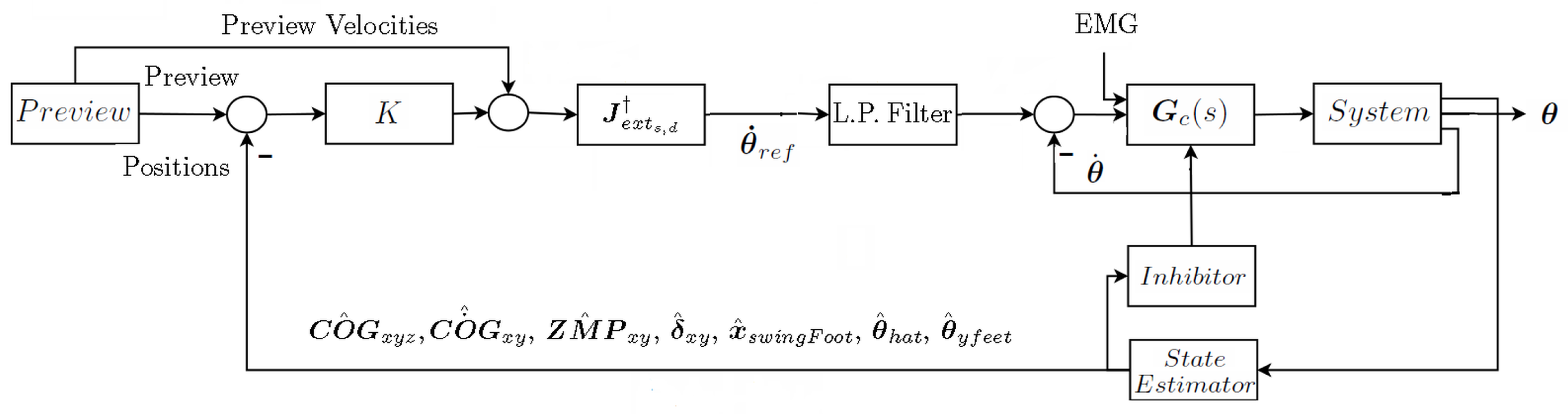
2.3. Closing the Loop

The feedback control is composed of two hierarchical loops: the internal one closed on the joint measures, the external one for gait, posture and equilibrium on the Cartesian space. The complete control scheme is depicted in Figure 5.
The internal loop, when the approach is used in an exoskeleton, receives along with input from equilibrium and postural tasks also the electromyographic signals for compliance with the patient. In this case, when the patient’s involuntary action brings the ZMP to the boundaries of the equilibrium region, an inhibitor block lowers the admittance gain to stop this action (see [1]).
The measures to close the external loop are joint angles, loads cells under the feet (CoP measures), inertial sensors on the trunk and on the feet for attitude and ultrasound sensors for the vertical position of the swing foot. The variables needed for the feedback are obtained by estimators fusing joint angles, through the kinematics of the system, with the other measures. Special attention is devoted to the critical COG/ZMP estimation and feedback gains to cope, especially, with modeling approximations. In this paper, an extended estimator based on a linearized inverted pendulum model is used. The content is outlined in Appendix A.
With these estimates, adopting an evolution of Choi’s approach to close the COG/ZMP loop and a simple PD scheme for the other variables, the following feedback is proposed, for single and double stance:
θ ˙ r e f i = J e x t i · ( V i + E i ) , i = s , d
wherein:
  • J e x t i is the pseudoinverse of the extended Jacobian matrix J e x t i , as described in Section 2.2;
  • Vi is the vector of the preview velocities and acts as feed-forward;
  • Es is a vector containing the feedback tracking errors, computed as the difference between the preview/reference and the estimates of the corresponding Cartesian variables.
Specifically, in single stance, the following expression holds:
E s = K C O G · e C O G + K C O ˙ G · e C O ˙ G K Z M P · e Z M P K C O G z · ( C O G z r e f C O ^ G z ) K h a t · ( θ h a t r e f θ ^ h a t ) K f e e t y · ( θ y f e e t r e f θ ^ y f e e t ) K f o o t · ( x s w i n g F o o t r e f x ^ s w i n g F o o t ) E k n e e s
where e C O G = C O G x y p r e v i e w ( C O ^ G x y + δ ^ x y ) , e C O ˙ G = C O ˙ G x y p r e v i e w C O ˙ ^ G x y , e Z M P = Z M P x y p r e v i e w ( Z M ^ P x y + δ ^ x y ) , and δ ^ x y is the estimate of the displacement of the theoretical Z M ^ P , resulting from the inverted pendulum model from the measured CoP, due to modeling approximations and internal or external force disturbances. The error Eknees, related to the knees, is discussed in the next section.
Similar expressions apply to the case of double stance, returning θ ˙ r e f d , where in the vectors Ed, and Vd, position errors and feedforward velocities relative to the swinging foot coordinates are not present.
Choi has proven, using Lyapunov techniques, that values of KCOG and KZMP, which stabilize a simple linearized inverted pendulum, always exist. This is correct; however, in practice, as the simulations show, the system is always poorly damped. Here, a much more effective approach is followed by computing a state feedback from the extended estimator of COG/ZMP described in Appendix A.
The control strategies in the left and right modes are identical, with just the joint angles of right and left legs being interchanged. A state machine, synchronized to gait events, switches the control strategy from single to double left/right stance according to a unitary control scheme.

2.3.1. Knee References

Note that, using extended Jacobian matrices, the knee reference velocities are present in the feedforward velocity vectors Vs, Vd in Equation (6). However, as the knee angles are not of primary importance and do not need to be tracked, knee tracking errors in Eknees assume a particular form. They are substituted by the negative of a filtered interpolation of the maximum values reached by the knee angles during one stride cycle. This allows the maxima to be kept close to zero (note that with the present angle convention, knee angles are always negatives, reaching, when fully stretched, their maximum value at zero) and also acts as a deterrent, to avoid overstretching during walk, due to the singularity. In fact, the control action is such as to avoid the maxima of the knee angles crossing a zero reference value.
E k n e e s = [ , K k n e e s · θ k n e e s m a x T ] T
where θ k n e e s m a x has components θ k n e e s m a x i θ k n e e s i ( t ) , i = 1 , 2 .

2.3.2. Filtering or Integrating θ ˙ r e f i , i = s , d

Two alternatives for the control have been tested: joint angles are closed in an internal joint velocity or a position loop. In the first case, the vector θ ˙ r e f i of Equation (6) is filtered by a low pass filter prior to being applied as a reference to the velocity loop. In the second case, the velocity vector is integrated to obtain the references for the position loop. In this case, it was found advantageous to improve stability, due to unmodeled actuator dynamics, to introduce a derivative action:
θ r e f i = ( 1 / s · I + K v ) θ ˙ r e f i
In the next example, as shown in Figure 5, the first alternative has been chosen.

2.3.3. Further Comments on the Extended Jacobian Matrix

The relationship that exists between COGz and θ k n e e 1 , θ k n e e 2 , and the over-dimensionality in the extended Jacobian matrices are now discussed in more detail.
Either assigning to the COGz a constant value or imposing an inverted pendulum walk to preserve energy, exploiting the over-dimensionality of the constraints and weighted least squares, it is possible to adopt a reference C O G z r e f slightly higher than what is needed. At the same time, that constraint is relaxed, choosing an appropriate weight for this component on the extended Jacobian. Therefore, the result is achieved to obtain an erect posture during gait at the maximum admissible height (the body is pulled by the feedback toward the erect posture), leaving a certain freedom of the COGz to accommodate uncertainties in walking.
It is emphasized that this solution can be extended to other independent joints (in addition to the knees), by adding other redundant constraints and using weighted least squares to overcome discrepancies arising from the reduced number of degrees of freedom of the model and simplified, sometimes arbitrarily, imposed trajectories. This is expected to add robustness to the control.

3. Reaction Force Control of the Feet

In double stance, the system is over-actuated. In Expressions (21) and (22) in Part I, the joint torques needed for position control were indicated as Tpos and the redundant as Taux. The reaction forces and torques F f o o t i of (23) in Part I, obtained by resolving the non-holonomic constraints, and given by Autolev, assume the form:
F f o o t 1 F f o o t 2 = G 1 ( θ d ) G 2 ( θ d ) · g + N l 1 ( θ d , θ ˙ d ) N l 2 ( θ d , θ ˙ d ) + J 1 ( θ d ) J 2 ( θ d ) · θ d ¨ + M 1 p o s M 1 a u x M 2 p o s M 2 a u x · T p o s T a u x
Most of the terms present in Equation (10) are imposed by the motion, but in particular, F f o o t 1 and F f o o t 2 are linearly dependent through M 1 a u x and M 2 a u x on Taux, which is free.

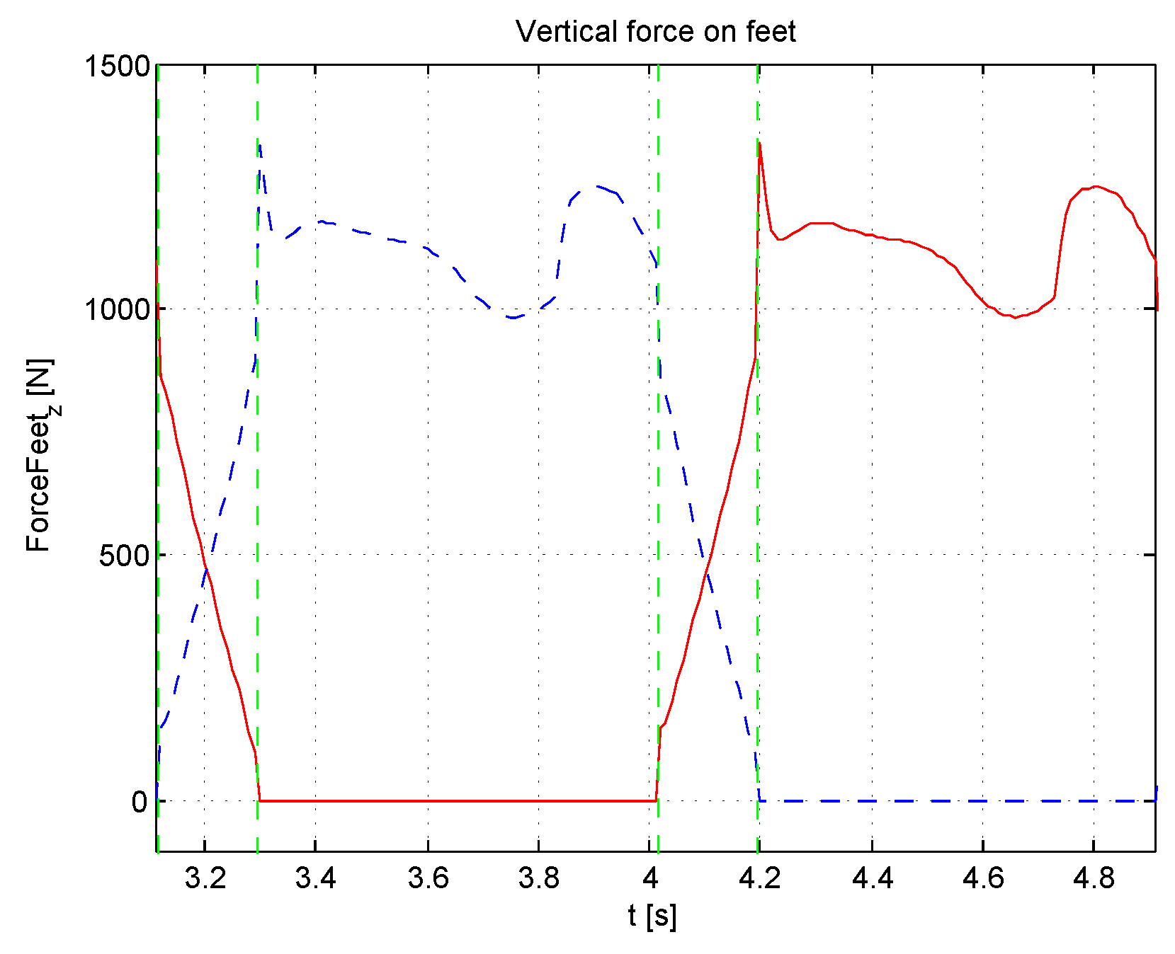
3.1. Balancing Weight

The 10 ground reaction forces/torques on the two feet cannot assume arbitrary values (rotation along z has been constrained, because of the straight walk), as their sum depends on the imposed motion, but their ratio can be controlled by the five components of Taux. Let the desired reference values of these reactions’ forces/torques on each foot, during a double stance phase, perform the transfer of weight from foot1 to foot2:
F f o o t 1 r e f = ( F f o o t 1 + F f o o t 2 ) · ( 1 α ) F f o o t 2 r e f = ( F f o o t 1 + F f o o t 2 ) · α , 0 α 1
This is achieved moving α from zero to one, and, in particular, α = 0.5 is the center balance.
The difference of the errors between references and actual values is given by:
e 1 e 2 = ( F foot 1 r e f F f o o t 1 ) ( F foot 2 r e f F f o o t 2 ) = = ( F f o o t 1 + F f o o t 2 ) · ( 1 2 α ) ( F f o o t 1 F f o o t 2 )
It can be controlled by Taux, considering that F f o o t 1 + F f o o t 2 is given by the motion, but:
F f o o t 1 F f o o t 2 ( M 1 a u x M 2 a u x ) · T a u x
and information on e 1 e 2 is obtained from F f o o t 1 and F f o o t 2 measured through load cells on the soles of the feet ( ( e 1 e 2 ) m ).
Then, transferring the load from one foot to the other can be achieved by minimizing in real time ( e 1 e 2 ) m controlling Taux with a gradient technique based on the following iterative scheme:
T a u x ( t + Δ ) = T a u x ( t ) + ( M T · M ) 1 M T · k · ( e 1 ( t ) e 2 ( t ) ) m
where M = M 1 a u x M 2 a u x .
The choice of a value of the feedback gain k that offers stability was found from experiments not to be critical. The recursion converges, and reaction forces/torques under the feet behave properly, tracking the desired reference. This will be particularly evident in the case study presented in the next section, where a linear transition of the transfer of weight has been imposed.

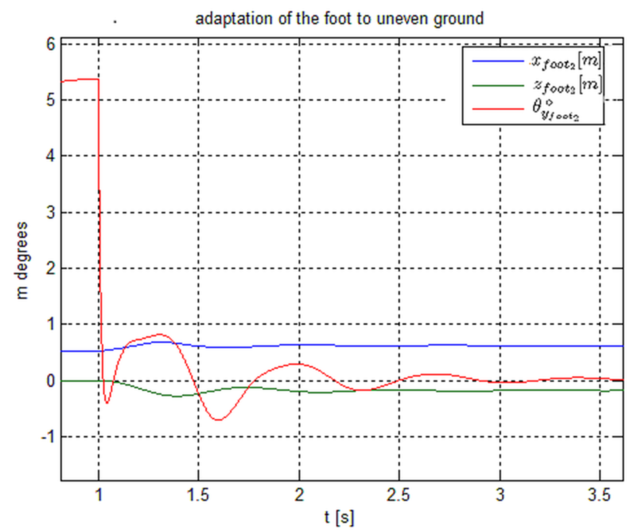
3.2. Adapting the Swing Foot on Uneven Ground at the End of a Single Stance

Taux and the second equation of Equation (10) are, also, exploited to offer compliance with the collision of the swing foot at the end of a single stance phase and to adapt the foot to uneven soil, before initiating the transfer of weight. The idea is the following:
  • the switching of the control from single to double stance is anticipated with respect to the event Heel2 strike of an interval of time compatible with the time response of the joint actuators.
  • The small adjustments of the swing foot in the instants just before and after the contact, during the adaptation, are ignored by the postural control, which treats them as disturbances.
  • A virtual force/torque is imagined as being applied to the swing foot (still flying) with a desired spring admittance ( F m = k · x + β · x ˙ ) attracting the foot toward the real future contact position and soil attitude that have just been measured. They may have slightly different values than those of the reference trajectory planned in advance.
  • The reaction force control for F f o o t 2 is activated, acting on Taux with a scheme similar to Equation (14), driven by the virtual force/torque before the contact, and then, after the contact by the real ones, with the objective to home to the contact point and adapting the foot to the ground by bringing reaction forces/torques to a minimum.
This case is a little different than simply weight transferring, because a small motion (with its dynamics) is still involved, and convergence of the recursion (i.e., stability of the force feedback) is more critical. For this, instead of the simple discrete integrator of Equation (14), an integrator with a derivative action of the type of I(s) = k · (s + z)/s has been necessary:
x ( t + Δ ) = A · x ( t ) + B · u ( t ) T a u x ( t ) = C · x ( t ) + D · u ( t ) u ( t ) = ( M 2 a u x T · M 2 a u x ) 1 M 2 a u x T · F m ( t )
The next Figure 6 shows the particulars of the transition from the position to force control of the swing foot before contact in the presence of a discrepancy between the planned arrival point and the real one.
How to compute and monitor the impulse generated by the impact and the discontinuity in the values of the generalized speeds is discussed in Part I. [27].

4. The Case Study

In this example, the patient and the exoskeleton together of [1] are simulated. No independent dynamics is assumed for the patient; however, discrepancies of the system with respect to a simple inverted pendulum on which is based the equilibrium control are taken into account, as a disturbance, in the extended estimator of COG/ZMP. The simulator and gait details are described in Part I. A rectilinear gait of a few strides, starting and ending with a hold position with the center of balance, has been simulated.
An extended Jacobian was adopted with a nominal standard trajectory for the knees taken from [28,29] and a very small weighting factor (0.2) with respect to one for the other variables. This is sufficient to avoid singularities, allowing the knee angles to be controlled at the extremes, leaving the behavior of the knees to adapt to the actual situation without strictly following the nominal trajectories. It can be seen in Figure 7, where left and right knee angle trajectories are presented.
Physiologically, an overstretching of the knees of a few degrees is normal. It has also been allowed in the simulation to show how the singularity was handled by this approach. However, by increasing Kknees, it could have been easily prevented.
In the present case study, the control sampling time is 1 ms. The internal joint loop is controlled in velocity, with a speed gain of k = 1000. The other gains are K C O G = 5 , K C O ˙ G = 0.25 , K Z M P = 0.05 , K f o o t = 5 , K h a t = 0.5 , K C O G z = 10 , K f e e t y = 5 , K k n e e s = 1 .
In Figure 8, the reference (dashed) and simulated COG and ZMP in the sagittal and frontal planes are shown. The reference of COGz is taken as constant. The indication of the transitions between single/double stances is superimposed.
The reaction forces and torques on the feet are presented in Figure 9 and Figure 10. In particular, the torques on feet around the y axis represent the control of active toes, while heel joints are passive in this example. Interestingly, during the first part of the single stance, the torque is given by the flat foot on the ground; in the second part, after Heel1 off, it needs the active contribution of the joint on toe1. Maintaining the supporting foot flat for the entire single stance period, i.e., moving the event Heel1 off to be coincident with Heel2 strike, could have avoided an active joint on the feet’s toes.
The angles of hips and ankles are in Figure 11, with torques applied to ankle, knee and hip joints in Figure 12.

5. Conclusions

The paper proposes a switching control system for a biped device during walking that approaches unitarily single and double stances. It is suitable for either lower limb exoskeletons or autonomous biped robots.
Particular attention has been devoted to over-actuation in double stance, exploited here for ground reaction force control for load transfer and switching the control from single to double stance immediately before actual contact, to ensure compliance for the adaptation of the swing foot to uneven soil.
By using Jacobian matrices to transfer trajectories from the Cartesian to the joint space, the adoption of an extended Jacobian and weighted least squares offers redundancy in the assignment of the constrains with several advantages:
  • to resolve the singularity in the inverse kinematics and allow the knees to be fully stretched, by introducing fake knee joint trajectories;
  • to accommodate kinematics inconsistency due to model and preview trajectories’ approximations;
  • to take into account the actions and style of the wearer, in the case of an exoskeleton with a partially able patient, ending up in a hybrid control system.
There is, however, one question that deserves further investigation and testing when the approach is used for an exoskeleton. Admittance control for compliance will offer partial freedom to the wearer, in the neighborhood of a nominal gait. However, the interaction between the present control loop and the patient’s instinctive reactions is unclear, i.e., the effect that the physiological human feedback loop will have on the system. This will be tested on the prototype exoskeleton that is being developed by the authors.
This Part II is limited to rectilinear walking, extensions to walking while turning are approached in Part III.
This research was originated from the European Patent No. EP 2.497.610.

Acknowledgments

This research has been partially supported by MIUR, the Italian Ministry of Instruction, University and Research, and from the Piedmont Region.

Author Contributions

The authors contributed equally to this work.

Conflicts of Interest

The authors declare no conflict of interest.

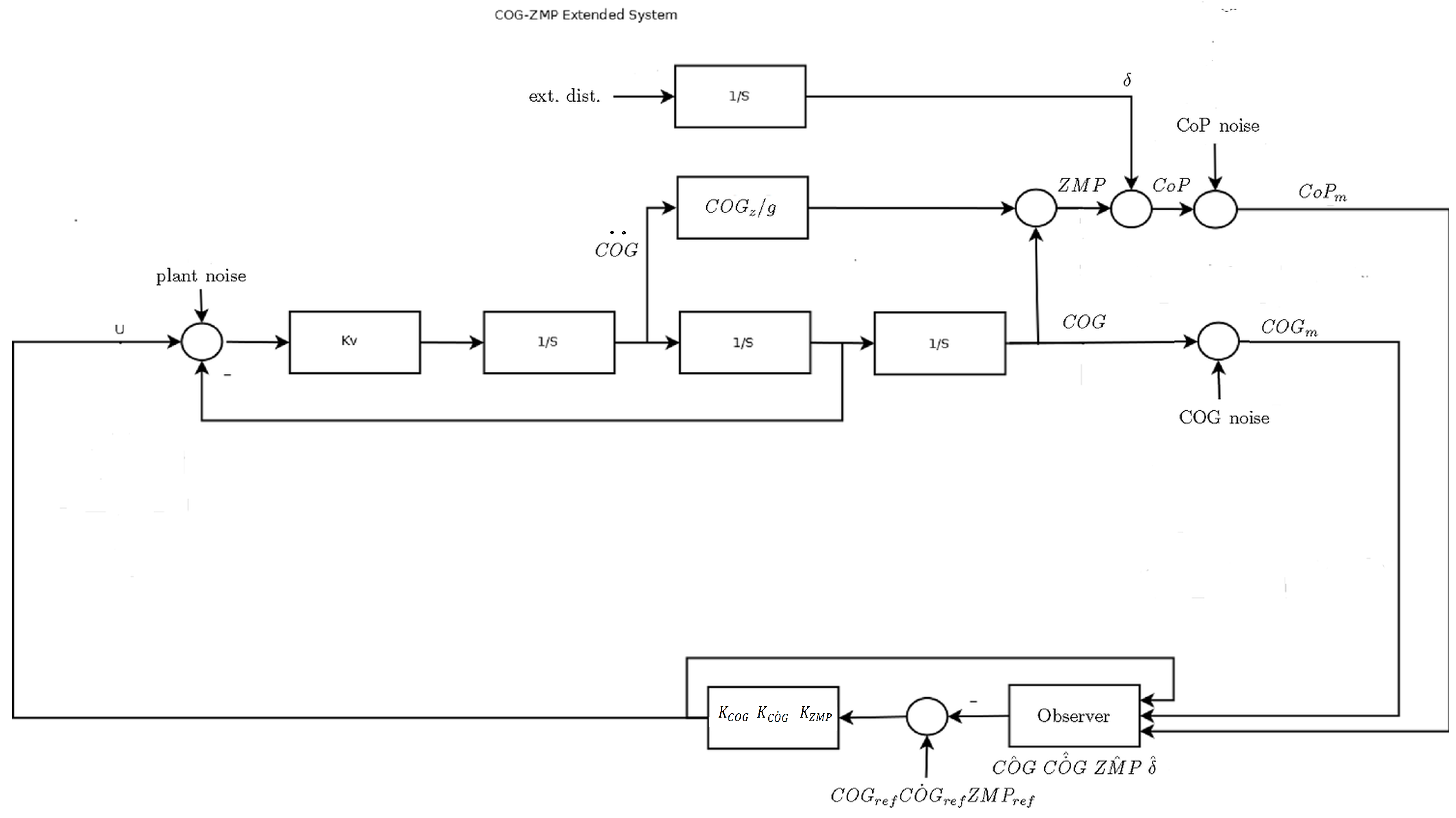
Appendix A. COG/ZMP Estimator and Control

The control of equilibrium is based on a linearized inverted pendulum model, while the real biped is not. Moreover, in the case of an exoskeleton, involuntary motions of the patient affect the COG and introduce internal or external (e.g., a crutch) forces to the system. In these conditions, the CoP measures under the feet and the theoretical (inverted pendulum) ZMP do not assume the same value. In order to fuse and make consistent joint measures, based on kinematics, with CoP measures, and to adopt a simple linearized inverted pendulum model for the estimator, discrepancies have to be accounted for. This is achieved in two steps.
  • As the weight distribution is seldom well known, especially in the case of an exoskeleton, an a priori calibration of the kinematics, with static and dynamic experiments, is suggested, adopting the same feet sensors that will be used for the control.
  • An extended estimator is introduced by adding in its simplest form one more state to the original model, to take into account the disturbances.
With this estimator C O ^ G x y , C O ˙ ^ G x y , Z M ^ P x y , δ ^ x y are obtained, where δ ^ x y estimates the discrepancy between ZMP and COP. The variables that must track the reference preview signals now become C O ^ G x y + δ ^ x y and Z M ^ P x y + δ ^ x y .
Moreover, considering that the joint actuators are driven by a speed control, together with the estimator, a feedback can be computed using LQGor H techniques. This is obtained by adding simplified speed actuator dynamics to the inverted pendulum model.
The complete model with the resulting control for each axis is shown in Figure A1. Details of the approach are described in [30]. Estimator and feedback gains are then adopted in the general motion control of Equation (7).
Figure A1. COG/ZMP estimator and control for one axis.
Inventions 01 00007 g013

References

  1. Menga, G.; Ghirardi, M. Lower Limb Exoskeleton with postural equilibrium enhancement for rehabilitation purposes. Internal Report DAUIN—Politecnico di Torino. Available online: https://dl.dropboxusercontent.com/u/26129003/SUBM1.pdf (accessed on 17 March 2016).
  2. Hirai, K.; Hirose, M.; Haikawa, Y.; Takenaka, T. The development of honda humanoid robot. In Proceedings of the 1998 IEEE International Conference on Robotics and Automation, Leuven, Belgium, 16–20 May 1998.
  3. Sakagami, Y.; Watanabe, R.; Aoyama, C.; Matsunaga, S.; Higaki, N.; Fujimura, K. The intelligent ASIMO: System overview and integration. In Proceedings of the IEEE/RSJ International Conference on Intelligent Robots and Systems, Lausanne Switzerland, October 2002; pp. 2478–2483.
  4. Endo, G.; Nakanishi, J.; Morimoto, J.; Cheng, G. Experimental studies of a neural oscillator for biped Locomotion with QRIO. In Proceedings of the 2005 IEEE International Conference on Robotics and Automation, Barcellona, Spain, 18–22 April 2005.
  5. Lohmeier, S.; Loffler, K.; Gienger, M.; Ulbrich, H.; Pfeiffer, F. Computer system and control of biped “Johnnie”. In Proceedings of the 2004 IEEE International Conference on Robotics and Automation, New Orleans, USA, 26 April–1 May 2004; pp. 4222–4227.
  6. Yokoi, K.; Kanehiro, F.; Kaneko, K.; Kajita, S.; Fujiwara, K.; Hirukawa, H. Experimental study of humanoid robot HRP-1S. Int. J. Robot. Res. 2004, 23, 351–362. [Google Scholar] [CrossRef]
  7. Park, I.W.; Kim, J.Y.; Lee, J.; Oh, J.H. Online free walking trajectory generation for biped humanoid robot HR-3(HUBO). In Proceedings of the 2006 IEEE International Conference on Robotics and Automation, Orlando, FL, USA, 15–19 May 2006.
  8. Sentis, L.; Khatib, O. Synthesis of whole-body behaviors through hierarchical control of behavioral primitives. Int. J. Humanoid Robot. 2005, 2, 505–518. [Google Scholar] [CrossRef]
  9. Choi, Y.; Kim, D.; Oh, Y.; You, B. Posture/walking control for humanoid robot based on kinematic resolution of CoM jacobian with embedded motion. IEEE Trans. Robot. 2007, 22, 1285–1293. [Google Scholar] [CrossRef]
  10. Sentis, L.; Park, J.; Khatib, O. Compliant control of multicontact and center-of-mass behaviors in humanoid robots. IEEE Trans. Robot. 2010, 26, 483–501. [Google Scholar] [CrossRef]
  11. Azevedo, C.; Poignet, P. Artificial locomotion control: From human to robots. Robot. Auton. Syst. 2004, 47, 203–223. [Google Scholar] [CrossRef]
  12. Vukobratovic, M. Humanoids robots: Past, present state, future. In Proceedings of the SISY—Serbian-Hungarian Joint Symposium on Intelligent Systems, Subotica, Serbia, 29–30 September 2006.
  13. Katayama, T.; Ohki, T.; Inoue, T.; Kato, T. Design of an optimal controller for a discrete time system subject to previewable demand. Int. J. Control 1985, 41, 677–699. [Google Scholar] [CrossRef]
  14. Yang, W.; Chong, N.Y.; Ra, S.; Kim, C.; You, B.J. Self-stabilizing bipedal locomotion employing neural oscillators. In Proceedings of the 2008 8th IEEE-RAS International Conference on Humanoid Robots, Daejeon, Korea, 1–3 December 2008.
  15. Righetti, L.; Ijspeert, A. Programmable central pattern generators: An application to biped locomotion control. In Proceedings of the IEEE International Conference on Robotics and Automation, Orlando, FL, USA, 15–19 May 2006.
  16. Kajita, S.; Espiau, B. Legged Robots; Springer Handbook of Robotics; Springer Berlin Heidelberg: Heidelberg, Germany, 2008; pp. 361–389. [Google Scholar]
  17. Hurmuzlu, Y.; Genot, F.; Brogliato, B. Modeling, stability and control of biped robots-a general framework. Automatica 2004, 40, 1647–1664. [Google Scholar] [CrossRef]
  18. Azevedo, C.; Espiau, B.; Amblard, B.; Assaiante, C. Bipedal locomotion; toward a unified concept in robotics and neuroscience. Biol. Cybern. 2007, 96, 209–228. [Google Scholar] [CrossRef] [PubMed]
  19. Siciliano, B.; Khatib, O. Springer Handbook of Robotics; Springer: Berlin, Germany; Heidelberg, Germany, 2008; Chapter 16. [Google Scholar]
  20. Kane, T.R.; Levinson, D.A. Dynamics: Theory and Applications; McGraw-Hill: New York, NY, USA, 1985. [Google Scholar]
  21. Kajita, S.; Kanehiro, F.; Kaneko, K.; Fujiwara, K.; Harada, K.; Yokoi, K.; Hirukawa, H. Biped walking pattern generation by using preview control of zero-moment point. In Proceedings of the 2003 IEEE International Conference on Robotics and Automation, Taipei, Taiwan, 14–19 September 2003.
  22. Yamane, K.; Nakamura, Y. Natural motion animation through constraining and deconstraining at will. IEEE Trans. Vis. Comput. Graph. 2003, 9, 352–360. [Google Scholar] [CrossRef]
  23. Saunders, J.B.; Inman, V.T.; Eberhardt, D.H. The major determinants in normal and pathological gait. J. Bone Joint Surg. 1953, 35-A, 543–558. [Google Scholar] [PubMed]
  24. Ortega, J.; Farley, C.T. Minimizing center of mass vertical movement increases metabolic cost in walking. J. Appl. Physiol. 2005, 99, 2099–2107. [Google Scholar] [CrossRef] [PubMed]
  25. Srinivasan, M.; Ruina, A. Idealized walking and running gaits minimize work. Proc. R. Soc. A 2007, 463, 2429–2446. [Google Scholar] [CrossRef]
  26. Kuo, A. The six determinants of gait and the inverted pendulum analogy: A dynamic walking perspective. Hum. Mov. Sci. 2007, 26, 617–56. [Google Scholar] [CrossRef] [PubMed]
  27. Menga, G.; Ghirardi, M. Modeling, Simulation and Control of the Walking of Biped Robotic Devices—Part I: Modeling and Simulation using Autolev. Inventions 2016, 1, 6. [Google Scholar]
  28. Patton, J. Normal Gait Part of Kinesiology. 2002. Available online: http://www.smpp.northwestern.edu/~jim/kinesiology/partA_introGait.ppt.pdf (accessed on 17 March 2016).
  29. Patton, J. Gait Section, Part B, Kinesiology. Available online: http://www.smpp.northwestern.edu/~jim/kinesiology/partB_GaitMechanics.ppt.pdf (accessed on 17 March 2016).
  30. Menga, G.; Ghirardi, M. Estimation and Closed Loop Control of COG/ZMP in Biped Devices Blending CoP Measures and Kinematic Information. Internal Report DAUIN—Politecnico di Torino. Available online: https://dl.dropboxusercontent.com/u/26129003/COGZMP.pdf (accessed on 17 March 2016).
Figure 1. (Left) Sagittal plane preview C O G x p r e v i e w (dashed blue) and Z M P x p r e v i e w (red); (right) frontal plane preview C O G y p r e v i e w (dashed blue) and Z M P y p r e v i e w (red).
Inventions 01 00007 g001
Figure 2. θ y f e e t r e f (left), θ ˙ y f e e t r e f (right): behavior of the angles and the speeds of the feet (red = left foot; blue = right foot), with superimposed stance phase (black).
Inventions 01 00007 g002
Figure 3. (Left) x s w i n g F o o t r e f , x ˙ s w i n g F o o t r e f , progression along x of the swing foot; (right) z s w i n g F o o t r e f , z ˙ s w i n g F o o t r e f , raising the swing foot.
Inventions 01 00007 g003
Figure 4. (Left) θ k n e e 1 r e f (red) and θ k n e e 2 r e f (blue dashed), references of the knee angles from [28,29]; (right) the corresponding velocities.
Inventions 01 00007 g004
Figure 5. The complete control scheme of equilibrium and posture.
Inventions 01 00007 g005
Figure 6. x, z, θ behavior of a swing foot switching from position to force control just before the contact. Discrepancies are 0.1 m on the position and 5° on the angle.
Inventions 01 00007 g006
Figure 7. (Left) A stride of the simulation on the sagittal plane; (right) reference (dashed) and actual (solid) knees angles during one stride (blue = left leg; red = right leg).
Inventions 01 00007 g007
Figure 8. Reference (dashed) and actual (solid) Center of gravity (COG, blue) and zero moment point (ZMP, red).
Inventions 01 00007 g008
Figure 9. Vertical reaction forces on feet (dashed blue = left foot, solid red = right foot). Green vertical lines represent stance changes.
Inventions 01 00007 g009
Figure 10. Frontal and sagittal reaction forces and torques on feet (dashed blue = left foot, solid red = right foot). Green vertical lines represent stance changes.
Inventions 01 00007 g010
Figure 11. Joint angles (dashed blue = left foot, solid red = right foot). Green vertical lines represent stance changes.
Inventions 01 00007 g011
Figure 12. Joint torques (dashed blue = left foot, solid red = right foot). Green vertical lines represent stance changes.
Inventions 01 00007 g012

