Modelling, Simulation and Control of the Walking of Biped Robotic Devices—Part I : Modelling and Simulation Using Autolev

Abstract

A biped robot is a mechanical multichain system. The peculiar features, that distinguishes this kind of robot with respect to others, e.g., industrial robots, is its switching nature between different phases, each one is the same mechanics subject to a different constraint. Moreover, because these (unilateral) constraints, represented by the contact between the foot/feet and the ground, play a fundamental role for maintaining the postural equilibrium during the gait, forces and torques returned must be continuously monitored, as they pose stringent conditions to the trajectories that the joints of the robot can safely follow. The advantages of using the Kane’s method to approach the dynamical model (models) of the system are outlined. This paper, divided in three parts, deals with a generical biped device, which can be an exoskeleton for rehabilitation or an indipendent robot. Part I is devoted to modelling and simulation, part II approaches the control of walk in a rectilinear trajectory, part III extends the results on turning while walking. In particular, this part I describes the model of the biped robot and the practicalities of building a computer simulator, leveraging on the facilities offered by the symbolic computational environment Autolev that complements the Kane’s method.

1. Introduction

A biped robot is a particular mechanical multichain system, which, as the time evolves, switches between phases (single stance, double stance, each one divided by subphases), characterized by different constraints. This has several consequences:

From a postural equilibrium point of view because these (unilateral) constraints, represented by the contact between the foot/feet and the ground, play a fundamental role for maintaining the postural equilibrium during the gait, their returned forces and torques pose stringent conditions to the trajectories that the joints of the robot can safely follow, and must be continuously monitored;

From the robot control point of view the changing constraints modify the number of degrees of freedom (DOF) of the dynamics, that can result underactuaded or overactuaded depending on the ground contacts, and the controller itself must be a switching system.

The authors have been involved for several years in modelling and control of biped robots for entertainment [1] and exoskeletons for postural rehabilitation [2], so they were faced from the beginning with the problem to provide the different projects with a reliable simulator. Commercial products such as ADAMS [3] were considered too limited from several points of view:

• the need to build an hybrid system switching among several phases;
• obtaining from the non-linear dynamical equations matrices of the linearized model to be used for designing a (linear) control;
• deriving explicitly computer code for the expressions of Jacobians matrices, kinematics, and in general of mechanical quantities needed for analysis and then to be embedded in the control;
• obtaining from the ground constraint the theoretical expressions of reaction forces/torques on the feet needed to evaluate the postural equilibrium, to balance the weight and offer compliance to the swing foot in the contact with the ground.

For these reasons the approach to build a completely open simulator, with full control of the programming was pursued.

Hybrid complementarity dynamical systems [4,5] model the behaviour of biped robots during walk. They are the basis of the control of bipeds through forward dynamics (see [6] section 16.3). These models correctly treat the contact between the ground and the feet as unilateral constraints. We follow here a different approach by considering the contact as a bilateral constraint and describing the system as different non-holonomic dynamical models, one for each phase of the gait. This has, with respect to classical approaches, some advantages: the models are simpler, as they don’t require the iterative computation of lagrangian multipliers needed to solve the constraints, they explicitly show for each phase the degrees of freedom of the dynamics, allowing to choose independent and depend control variables, and offering analitically reaction forces and torques at the ground. However, this approximation has one drawback: these models can handle patological walking situations of slipping or detachment of the foot from the ground only indirectly. To take full advantage of the approach, instead of the standard equations proposed in the literature the Kane’s method [7] has been adopted in order to derive the multi-chain dynamics. This method was originated in the spacecraft dynamics community, and apparently is not widely known in the robotic, and particularly biped robotic field, yet. A primer of the method will be given in one of the next sections, but just as introduction one of its advantages, with respect to other methods, is the capability to derive unitarily from the biped free in the space the several lower order non-holonomic representations in the presence of different constraints. For a more detailed discussion on simulators of multibody chains, specifically using the Kane’s method see [8]. Moreover the Kane’s method is complemented with a symbolic computational environment, originally called Autolev and now MotionGenesis Kane 5.x [9], that generates all mathematical expressions needed for modelling and design controls, and produces prototypical source code in Fortran, Matlab or C of the equations in ordinary differential form (ODEs) even for non holonomical constrained systems, which can be simulated using standard solvers.

In this framework are easily available, also, expressions of a variety of mechanical quantities needed for the analysis, such as linearization matrices, kinematics, Jacobians, explicit reaction forces/torques from the constraints, kinetic energy, generalized impulses, generalized momentum, etc.

The fragments of C software generated by Autolev have been casted, with few small modifications, into a framework of Object Oriented Design in C++ obtaining the hybrid nonlinear system simulation we needed and an easy interface with control modules and reference trajectory generators. Moreover, some of the mathematical expressions present in the model can be extracted from the simulator and in the future embedded in the real time hardware to become integral part of the control.

This paper extends the study of a lower limb exoskeleton for postural rehabilitation [2] and is composed by three parts. This first part is devoted to modelling and simulation, part II approaches the control of walk in a rectilinear trajectory, part III extends the results on turning while walking.

The organization of Part I is as follows: a review of previous work, specifically hybrid complementary dynamical systems, is presented in Section 2; in Section 3 a biped robot and its mechanical model is described; in Section 4 the general scheme of the simulator is presented.

2. Hybrid Complementarity Dynamical Systems

A small review of these models is taken from the related literature [10,11,12,13].

A biped robot is a three-dimension rigid multichain. Basically, the internal configuration variables ${\mathbf{q}}_1$ are the ones of the joint space Q. However, it is usual to consider a walking robot as a system free in the space, but subject to non-constant unilateral constraints. Hence, the configuration space is $Q\oplus {\mathbb{R}}^6$, where the six dimensional displacement of a given body is parameterized by ${\mathbf{q}}_2$. Assuming that the body structure is rigid, continuous dynamics can be expressed under the following Lagrangian form

$$\mathbf{M}\left(\mathbf{q}\right)·\ddot{\mathbf{q}}+\mathbf{C}(\mathbf{q},\dot{\mathbf{q}})·\dot{\mathbf{q}}+\mathbf{G}\left(\mathbf{q}\right)=\mathbf{\Gamma }(\mathbf{q},\dot{\mathbf{q}},\mathit{\tau })+{\mathbf{\Gamma }}_{ext},$$

(1)

where $\mathbf{q}={({\mathbf{q}}_1,{\mathbf{q}}_2)}^T\in {\mathbb{R}}^n$ is the parametrization vector of the whole configuration space of the biped considered as free in 3D space, $\mathbf{\Gamma }\in {\mathbb{R}}^n$ is the generalized efforts vector (function of the joint actuation torque $\mathit{\tau }\in {\mathbb{R}}^m$), $\mathbf{M}$ is the inertia matrix, $\mathbf{C}$ are the centrifugal, gyroscopic, and Coriolis contribution, and $\mathbf{G}$ is the generalized gravity force vector. Note that the set $(\mathbf{q},\dot{\mathbf{q}})$ constitutes the state of the biped, in the sense of the theory of dynamic systems. ${\mathbf{\Gamma }}_{ext}$ are torques generated by external reactions (ground contacts, interaction with objects) and they can be expressed as follows:

$${\mathbf{\Gamma }}_{ext}=\mathbf{J}{\left(\mathbf{q}\right)}^T·\mathit{\lambda }(\mathbf{q},\dot{\mathbf{q}})$$

(2)

where $\mathbf{J}\left(\mathbf{q}\right)$ is the Jacobian matrix of the points of the biped to which the external forces are applied and $\mathit{\lambda }(\mathbf{q},\dot{\mathbf{q}})$ are the Lagrangian multipliers corresponding to the amplitudes of these reactions.

The vector λ can be split in:

$$\mathit{\lambda }={({\mathit{\lambda }}_n,{\mathit{\lambda }}_t)}^T$$

(3)

where ${\mathit{\lambda }}_n$ and ${\mathit{\lambda }}_t$ are the normal and tangential components of the reactions, respectively. ${\mathit{\lambda }}_n$ satisfies the complementarity condition

$${\mathit{\lambda }}_n^T·\mathit{f}\left(\mathbf{q}\right)=0,{\mathit{\lambda }}_n\ge 0,\mathit{f}\left(\mathbf{q}\right)\ge 0$$

(4)

with $\mathbf{J}\left(\mathbf{q}\right)=\{\mathsf{\partial }{f}_i\left(\mathbf{q}\right)/\mathsf{\partial }{q}_j\},i,j=1\cdots n$ and ${\mathit{\lambda }}_t$ the Coulomb’s friction condition for each component:

$$|{\lambda }_{t_i}|\le \mu {\lambda }_{n_i}$$

(5)

Moreover, switching from single to double stance, the impact and restitution law has to be considered in setting the initial condition for the next phase.

Note, from an implementation point of view, that during simulation λ has to be numerically evaluated iteratively.

3. A Biped Robot

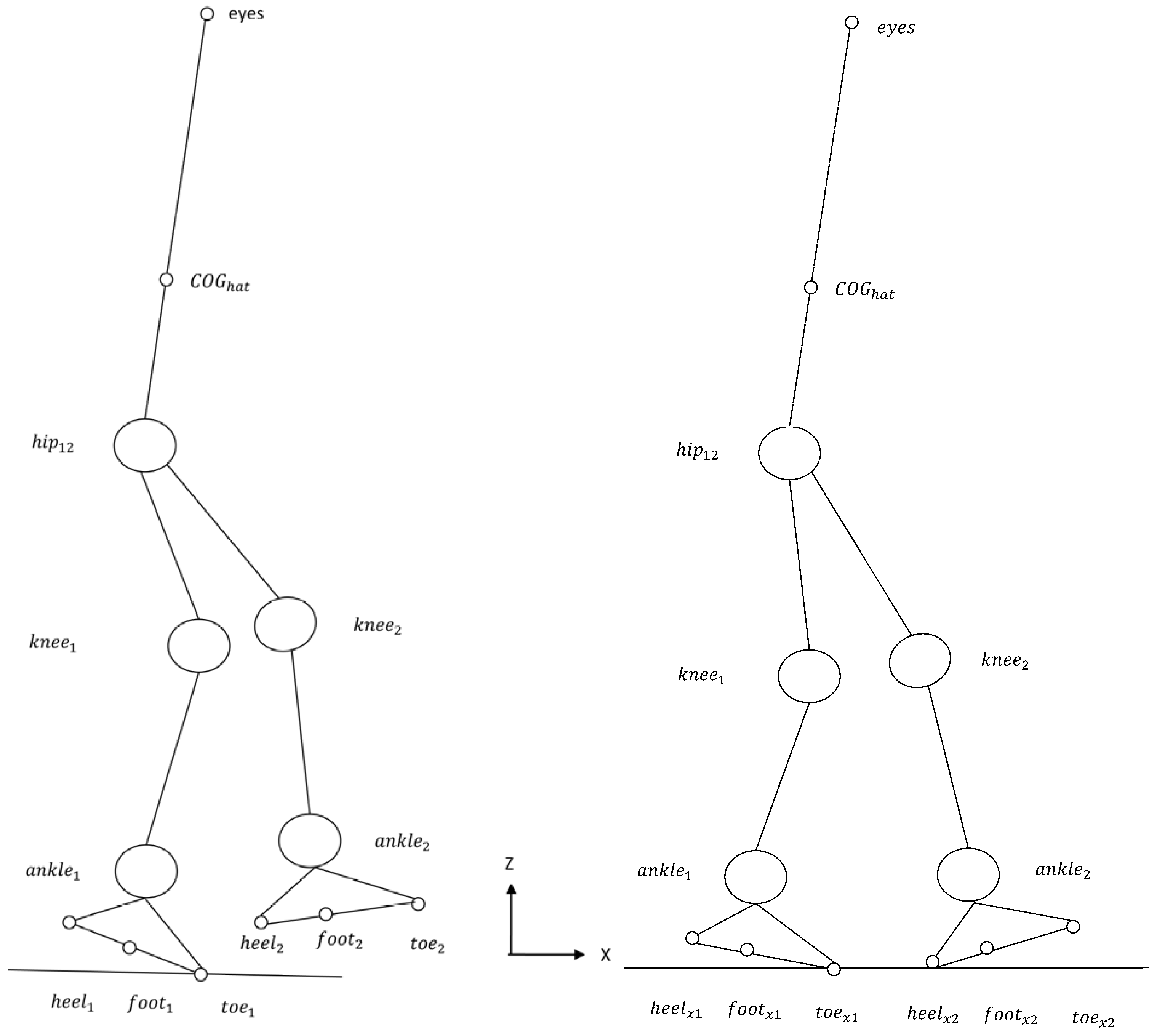
3.1. Mechanical Modelling

As it is known, the model of a multi-body system like a biped robot can be derived using different, essentially equivalent, methods. However, the ease of use of the various methods differs; some are more suited for multibody dynamics than others. The Newton-Euler method is comprehensive in that a complete solution for all the forces and dynamic variables are obtained, but it is inefficient. Applying the Newton-Euler method requires that force and moment balances be applied for each body taking in consideration every interactive and constraint force. Therefore, the method is inefficient when only a few of the system’s forces need to be solved for. Lagrange’s Equations provides a method for disregarding all interactive and constraint forces that do not perform work. The major disadvantage of this method is the need to differentiate scalar energy functions (kinetic and potential energy). This is not much of a problem for small multibody systems, but becomes an efficiency problem for large multibody systems.

In this work, instead, the so-called Kane’s method ([7]) has been chosen. This method is particularly interesting in this case because it is equally applicable to either holonomic or non-holonomic systems and, for non-holonomic systems, without the need to introduce Lagrangian multipliers. Briefly, the main contribution of the Kane’s method is that, through the concepts of motion variables (later called generalized speeds), the vectors of partial velocities and partial angular velocities, generalized active forces and generalized inertia forces, the dynamical equations are automatically determined, enabling forces and torques having no influence on the dynamics to be eliminated early in the analysis. Early elimination of these noncontributing forces and torques greatly simplifies the mathematics and enables problems having greater complexity to be handled. More into details:

Generalized coordinates and speeds A multi-body system, which possesses n degrees of freedom, is represented by a state with a n dimensional vector $\mathbf{q}$ of configuration variables (generalized coordinates) and an identical dimension vector $\mathbf{u}$ of generalized speeds called also motion variables, that could be any nonsingular combination of the time derivatives of the generalized coordinates that describe the configuration of a system. These are the kinematical differential equations:

$$u_r=\sum _{i=1,\cdots ,n}{Y}_{ri}\dot{q_i},r=1,\cdots ,n$$

(6)

$Y_{ri}$ may be in general nonlinear in the configuration variables so that the equations of motion can take on a particularly compact (and thus computationally efficient) form with the effective use of generalized speeds.

Partial velocities and angular velocities Partial velocities of each point (partial angular velocity of each body) are the n three-dimensional vectors expressing the velocities of that point (angular velocity of that body) as a linear combination of the generalized speeds. Let be ${\mathbf{v}}^P$ the translational velocity of a point P and ${\mathbf{\omega }}^B$ the rotational velocity of a body B with respect to the inertial reference frame, then

$$\begin{array}{c}{\mathbf{v}}^P=\sum _{r=1..n}{\mathbf{v}}_r^P{u}_r\\ {\mathbf{\omega }}^B=\sum _{r=1..n}{\mathbf{\omega }}_r^B{u}_r\end{array}$$

(7)

where ${\mathbf{v}}_r^P$ and ${\mathbf{\omega }}_r^B$ are the $r_{th}$ partial velocity and partial angular velocity of P and B, respectively.

Generalized active and inertia forces The n generalized forces acting on a system are constructed by the scalar product (projection) of all contributing forces and torques on the partial velocities and partial angular velocities of the points and bodies they are applied to.

Let us consider a system composed by N bodies $B_i$, where the torque ${\mathbf{T}}^{B_i}$, and force ${\mathbf{R}}^{P_i}$ applied to a point $P_i$ of $B_i$ are the equivalent resultant ("replacement" [7]) of all active forces and torques applied to $B_i$. Then

$$F_r^{B_i}={\mathbf{\omega }}_r^{B_i}·{{\mathbf{T}}_i}^{B_i}+{\mathbf{v}}_r^{P_i}·{\mathbf{R}}_r^{P_i}$$

(8)

is the $r_{th}$ generalized active force acting on $B_i$ and

$$F_r=\sum _{i=1,\cdots ,N}{F}_r^{B_i}$$

(9)

the $r_{th}$ generalized active force acting on the whole system. Identically for the inertia forces, indicated as $F_r^{*}$.

The dynamical equations for an n degree of freedom system are formed out from generalized active and inertial forces $F_r^{*}$

$$F_r+F_r^{*}=0,r=1,\cdots ,n.$$

(10)

These are known as Kane’s dynamical equations.

They result in a n dimensional system of second order differential equations ($2n$ order state variable representation) on generalized coordinates and speeds

$$\overline{\mathbf{M}}\left(\mathbf{q}\right)\dot{\mathbf{u}}+\overline{\mathbf{C}}(\mathbf{q},\mathbf{u})\mathbf{u}+\overline{\mathbf{G}}\left(\mathbf{q}\right)-\overline{\mathbf{\Gamma }}(\mathbf{q},\mathbf{u},\mathbf{\tau })=\mathbf{0},$$

(11)

where the parameter definitions are similar but not identical of Equation (1) and more efficient computationally [8].

Non-holonomic constraints When m constraints on the motion variables are added to the model, only $n-m$ generalized speeds are independents.The system is, then, called a non-holonomic system. The non-holonomic constraints are expressed as a set of m linear relationships between dependent and independent generalized speeds of the type

$$u_r=\sum _{i=1,\cdots ,p}{A}_{ri}{u}_i,r=p+1,\cdots ,n,$$

(12)

with $p=n-m$. In this case, selected the independent speeds, the Kane’s method immediately offers the minimal $2p$ order state variable representation from

$${\tilde{F}}_r+{\tilde{F}}_r^{*}=0,r=1,\cdots ,p,$$

(13)

where Kane calls ${\tilde{F}}_r$ and ${\tilde{F}}_r^{*}$ non-holonomic generalized active and inertial forces, while the remaining m original redundant equations resolve themselves in the expressions of the m reaction forces/torques returned by the constraints (because the Kane’s method is fundamentally based on the projection of forces on a tangent space on which the system dynamics are constrained to evolve, spanned by the partial velocities, reaction forces/torques result from the projection on its null-space).

Obviously, the choice of independent speeds is not unique, and they are usually found by inspection. However, a systematic way may be adopted considering that Equation (12) in the implicit vectorial form defines the null-space of $\mathit{u}$. Split $\mathit{u}$ in independent and dependent generalized speeds ${\mathit{u}}_1,{\mathit{u}}_2$ and rewrite Equation (12), introducing the matrix $\mathbf{A},pxm$, as

$$({\mathbf{A}}^T,-{\mathbf{I}}_{mxm})·\left[\begin{array}{c}{\mathit{u}}_1\\ {\mathit{u}}_2\end{array}\right]=0.$$

(14)

The columns of

$$\left[\begin{array}{c}\mathbf{A}\\ -{\mathbf{I}}_{mxm}\end{array}\right]$$

(15)

and

$$\left[\begin{array}{c}{\mathbf{I}}_{pxp}\\ {\mathbf{A}}^T\end{array}\right]$$

(16)

span, respectively null-space and range of $\mathbf{u}$. In order to obtain the most robust variables, permute the components of $\mathbf{u}$ in the independent generalized speeds so as to minimize the conditioning number of either equation (15) or (16).

Moreover, it is always possible to handle an holonomic (configuration) constraint as if it is non-holonomic, that is, to treat it as a motion constraint. This is particularly advantageous in biped robotics, in fact, considering foot/feet contact to the ground as non-holonomic contraints, from the reaction forces/torques returned from the constraint, the Zero Moment Point ($ZMP$) coordinates, and hence the Center of Pressure ($CoP$), can readily found as shown in the following subsection.

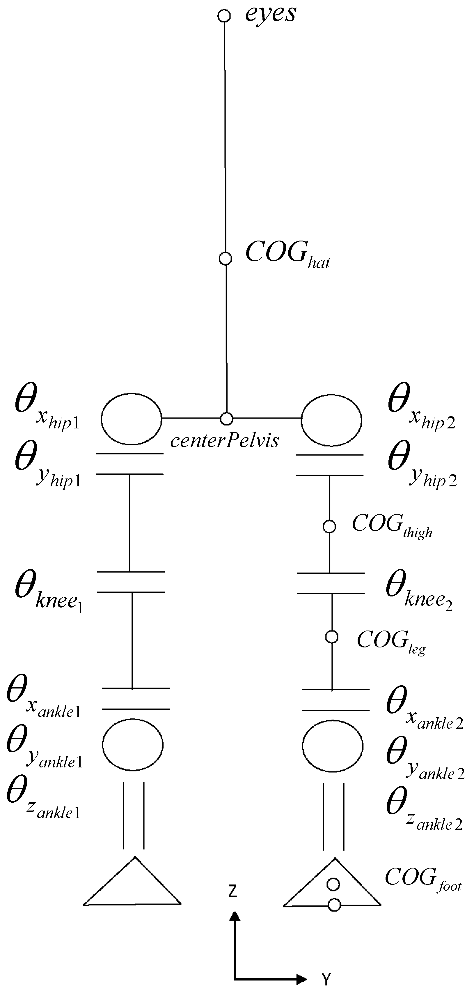
3.2. Robot Configuration

In this section the specific biped robotic structure we exploit in our practical applications in described. The key bodies and points are depicted in the Figure 1 and Figure 2 where the frontal and the sagittal view of the robot are depicted. It is composed of 7 bodies: feet, legs, thighs, hat (HAT: head, arm and trunk), connected by 12 joints: 2 ankles, 2 knees and 2 hips. Each ankle has 3 DOF, the knee 1 and the hip 2. In order to guarantee a natural gait the feet are allowed to rotate along y. This is equivalent to a hinge on the toes or on the heels of the foot/feet on the ground, resulting in 13 or 14 joints that can be potentially controlled, in single or double stance, respectively. In fact, to guarantee a human like walk it is mandatory that toe alone, or toe and heel joints are active [14,15,16].

Assuming the system free to move in the sagittal and frontal planes, but for simplicity not to rotate along the z axis (the walk is considered to be along a straight line without turns), it is characterized by 17 $DOF$ and an identical number of generalized variables and speeds, chosen here as the derivatives of the generalized variables. These are (angles are characterized by the rotation axis, the joint name and the limb index; positions by the axis, the point name and the limb index):

• The three positions on space of a reference point of $foo{t}_1$, were reaction forces are applied, taken at the center of the toe: $x_{to{e}_1},y_{to{e}_1},z_{to{e}_1}$.
• The two angles of the frame of foot 1: ${\theta }_{x_{foo{t}_1}},{\theta }_y{}_{foo{t}_1}$.
• The joint angles (as depicted in Figure 1): ${\theta }_{x_{ankl{e}_1}}$, ${\theta }_{y_{ankl{e}_1}}$,${\theta }_{z_{ankl{e}_1}}$, ${\theta }_{kne{e}_1}$, ${\theta }_{x_{hi{p}_1}}$, ${\theta }_{y_{hi{p}_1}}$, ${\theta }_{x_{hi{p}_2}}$, ${\theta }_{y_{hi{p}_2}}$, ${\theta }_{kne{e}_2}$, ${\theta }_{x_{ankl{e}_2}}$, ${\theta }_{y_{ankl{e}_2}}$ and ${\theta }_{z_{ankl{e}_2}}$.

Indicate with pedix 1 the right leg and pedix 2 the left leg, and use conventionally foot 1 as the supporting foot. The two configurations of single and double stance are defined as follows:

Single Stance: The exoskeleton is sustained by $foo{t}_1$. Both feet are allowed to rotate around y only, in particular $foo{t}_1$ is connected to the ground by a hinge at the $to{e}_1$ point, and it is imposed that the trunk is oriented straight ahead. Then, the three translational velocities of $to{e}_1$ ${\dot{x}}_{to{e}_1},{\dot{y}}_{to{e}_1},{\dot{z}}_{to{e}_1}$, the three rotational velocities ${\dot{\theta }}_{x_{foo{t}_1}}$, ${\dot{\theta }}_{x_{foo{t}_2}}$, ${\dot{\theta }}_{z_{foo{t}_2}}$ of both feet and the rotational velocity of the trunk ${\dot{\theta }}_{z_{hat}}$ are zero (motion constraints). In these conditions the system has 10 $DOF$ (7 have been constrained out of the original 17). The unique possible choices of independent generalized speeds is:

$$\begin{array}{cc}\hfill {\dot{\mathbf{\theta }}}_s=[& {\dot{\theta }}_{y_{foo{t}_1}},{\dot{\theta }}_{x_{ankl{e}_1}},{\dot{\theta }}_{y_{ankl{e}_1}},{\dot{\theta }}_{kne{e}_1},{\dot{\theta }}_{x_{hi{p}_1}},{\dot{\theta }}_{y_{hi{p}_1}},\hfill \\ & {\dot{\theta }}_{x_{hi{p}_2}},{\dot{\theta }}_{y_{hi{p}_2}},{\dot{\theta }}_{kne{e}_2},{\dot{\theta }}_{y_{ankl{e}_2}}{]}^T\hfill \end{array}$$

(17)

controlled by 10 torques at the corresponding joints

$$\begin{array}{cc}\hfill {\mathit{T}}_s=[& T_{y_{foo{t}_1}},T_{x_{ankl{e}_1}},T_{y_{ankl{e}_1}},T_{kne{e}_1},T_{x_{hi{p}_1}},T_{y_{hi{p}_1}},\hfill \\ & T_{x_{hi{p}_2}},T_{y_{hi{p}_2}},T_{kne{e}_2},T_{y_{ankl{e}_2}}{]}^T.\hfill \end{array}$$

(18)

Note that, if the toe of $foo{t}_1$ is passive we have an under-actuated system.

On the other hand, the motion constraints resolve themselves in 3 forces: $F_{x_{foo{t}_1}}$, $F_{y_{foo{t}_1}}$, $F_{z_{foo{t}_1}}$, and 4 torques: $T_{x_{foo{t}_1}}$, $T_{z_{ankl{e}_1}}$, $T_{x_{ankl{e}_2}}$, $T_{z_{ankl{e}_2}}$ of reaction. The first four, along with the control torque $T_{y_{foo{t}_1}}$, characterizing the foot reactions from the ground

$${\mathit{F}}_{foo{t}_1}={[F_{x_{foo{t}_1}},F_{y_{foo{t}_1}},F_{z_{foo{t}_1}},T_{x_{foo{t}_1}},T_{y_{foo{t}_1}}]}^T$$

(19)

are very important in determining the $ZMP$, the remaining three, vice versa, not essential for posture, will be ignored (The corresponding joints will be separately controlled with respect to the main multivariable control, in order to keep the biped trunk, as well as the swing foot, oriented straight ahead).

Double stance: when the exoskeleton is in double stance, both feet are on the ground. As they can rotate around y, it is assumed that $foo{t}_1$ is connected to the ground by a hinge, as before, at $to{e}_1$ and the $foo{t}_2$ at $hee{l}_2$, and the center of the heel ($x_{hee{l}_2},y_{hee{l}_2},z_{hee{l}_2}$) is the reference point where reaction forces are applied. Hence, the system loses 3 more degrees of freedom resulting in 7. There are four possible choices of independent generalized speeds, however, the best conditioned, according to Section 3.1, is:

$$\begin{array}{cc}\hfill {\dot{\mathbf{\theta }}}_d=[& {\dot{\theta }}_{y_{foo{t}_1}},{\dot{\theta }}_{x_{ankl{e}_1}},{\dot{\theta }}_{y_{ankl{e}_1}},{\dot{\theta }}_{kne{e}_1},{\dot{\theta }}_{y_{hi{p}_1}},\hfill \\ & {\dot{\theta }}_{kne{e}_2},{\dot{\theta }}_{y_{ankl{e}_2}}{]}^T\hfill \end{array}$$

(20)

and the system in this condition is controlled by the 7 torques at the corresponding joints

$$\begin{array}{cc}\hfill {\mathit{T}}_d=[& T_{y_{foo{t}_1}},T_{x_{ankl{e}_1}},T_{y_{ankl{e}_1}},T_{kne{e}_1},T_{y_{hi{p}_1}},\hfill \\ & T_{kne{e}_2},T_{y_{ankl{e}_2}}{]}^T.\hfill \end{array}$$

(21)

Note that the remaining 5 torques, comprehensive of $T_{y_{foo{t}_2}}$ at the hinge of $hee{l}_2$, if it is active,

$${\mathit{T}}_{aux}={[T_{x_{hi{p}_1}},T_{x_{hi{p}_2}},T_{y_{hi{p}_2}},T_{x_{ankl{e}_2}},T_{y_{foo{t}_2}}]}^T.$$

(22)

are redundant for position control. $T_{x_{ankl{e}_2}}$, which is irrelevant in single stance, along with the whole vector Equation (22), will play a significant role in load balance in double.

The complete list of the motion variables, constraints, reaction forces and torques, joint torques needed for position control, and redundant joint torques for single and double stance are contained in

Table 1. Single Stance.

Motion	Constraints	Reactions	Position	Free
Variables			Control	Forces/Torques
${\dot{\theta }}_{y_{foo{t}_1}}$			$T_{y_{foo{t}_1}}$	$F_{x_{foo{t}_2}}$
${\dot{\theta }}_{y_{ankl{e}_1}}$			$T_{y_{ankl{e}_1}}$	$F_{y_{foo{t}_2}}$
${\dot{\theta }}_{kne{e}_1}$			$T_{kne{e}_1}$	$F_{z_{foo{t}_2}}$
${\dot{\theta }}_{y_{hi{p}_1}}$			$T_{y_{hi{p}_1}}$	$T_{x_{foo{t}_2}}$
${\dot{\theta }}_{y_{hi{p}_2}}$			$T_{y_{hi{p}_2}}$	$T_{y_{foo{t}_2}}$
${\dot{\theta }}_{kne{e}_2}$			$T_{kne{e}_2}$	$T_{z_{foo{t}_2}}$
${\dot{\theta }}_{y_{ankl{e}_2}}$			$T_{y_{ankl{e}_2}}$
${\dot{\theta }}_{x_{ankl{e}_1}}$			$T_{x_{ankl{e}_1}}$
${\dot{\theta }}_{x_{hi{p}_1}}$			$T_{x_{hi{p}_1}}$
${\dot{\theta }}_{x_{hi{p}_2}}$			$T_{x_{hi{p}_2}}$
${\dot{\theta }}_{x_{ankl{e}_2}}$	${\dot{\theta }}_{xfoo{t}_2}$	$T_{x_{ankl{e}_2}}$
${\dot{\theta }}_{z_{ankl{e}_1}}$	${\dot{\theta }}_{z_{hat}}$	$T_{z_{ankl{e}_1}}$
${\dot{\theta }}_{z_{ankl{e}_2}}$	${\dot{\theta }}_{z_{foo{t}_2}}$	$T_{z_{ankl{e}_2}}$
${\dot{\theta }}_{x_{foo{t}_1}}$	${\dot{\theta }}_{x_{foo{t}_1}}$	$T_{x_{foo{t}_1}}$
${\dot{x}}_{to{e}_1}$	${\dot{x}}_{to{e}_1}$	$F_{x_{foo{t}_1}}$
${\dot{y}}_{to{e}_1}$	${\dot{y}}_{to{e}_1}$	$F_{y_{foo{t}_1}}$
${\dot{z}}_{to{e}_1}$	${\dot{z}}_{to{e}_1}$	$F_{z_{foo{t}_1}}$

and

Table 2. Double Stance.

Motion	Constraints	Reactions	Position	Free
Variables			Control	Forces/Torques
${\dot{\theta }}_{y_{foo{t}_1}}$			$T_{y_{foo{t}_1}}$
${\dot{\theta }}_{y_{ankl{e}_1}}$			$T_{y_{ankl{e}_1}}$
${\dot{\theta }}_{kne{e}_1}$			$T_{kne{e}_1}$
${\dot{\theta }}_{y_{hi{p}_1}}$			$T_{y_{hi{p}_1}}$
${\dot{\theta }}_{y_{hi{p}_2}}$	${\dot{x}}_{hee{l}_2}$	$F_{x_{foo{t}_2}}$		$T_{y_{hi{p}_2}}$
${\dot{\theta }}_{kne{e}_2}$			$T_{kne{e}_2}$
${\dot{\theta }}_{y_{ankl{e}_2}}$			$T_{y_{ankl{e}_2}}$
${\dot{\theta }}_{x_{ankl{e}_1}}$			$T_{x_{ankl{e}_1}}$
${\dot{\theta }}_{x_{hi{p}_1}}$	${\dot{z}}_{hee{l}_2}$	$F_{z_{foo{t}_2}}$		$T_{x_{hi{p}_1}}$
${\dot{\theta }}_{x_{hi{p}_2}}$	${\dot{y}}_{hee{l}_2}$	$F_{y_{foo{t}_2}}$		$T_{x_{hi{p}_2}}$
${\dot{\theta }}_{x_{ankl{e}_2}}$	${\dot{\theta }}_{x_{foo{t}_2}}$	$T_{x_{foo{t}_2}}$		$T_{x_{ankl{e}_2}}$
${\dot{\theta }}_{z_{ankl{e}_1}}$	${\dot{z}}_{hat}$	$T_{z_{ankl{e}_1}}$
${\dot{\theta }}_{z_{ankl{e}_2}}$	${\dot{\theta }}_{z_{foo{t}_2}}$	$T_{z_{ankle2}}$
${\dot{\theta }}_{x_{foo{t}_1}}$	${\dot{\theta }}_{x_{foo{t}_1}}$	$T_{x_{foo{t}_1}}$
${\dot{x}}_{to{e}_1}$	${\dot{x}}_{to{e}_1}$	$F_{x_{foo{t}_1}}$
${\dot{y}}_{to{e}_1}$	${\dot{y}}_{to{e}_1}$	$F_{y_{foo{t}_1}}$
${\dot{z}}_{to{e}_1}$	${\dot{z}}_{to{e}_1}$	$F_{z_{foo{t}_1}}$
				$T_{y_{foo{t}_2}}$

.

Reaction and control force/torques at the foot/feet are particularly important in biped robotics:

$${\mathit{F}}_{foo{t}_i}={[F_{x_{foo{t}_i}},F_{y_{foo{t}_i}},F_{z_{foo{t}_i}},T_{x_{foo{t}_i}},T_{y_{foo{t}_i}}]}^T$$

(23)

where $i=1,2$ and, specifically, the $CoP$ coordinates, derived from the $ZMP$, result in:

$$\begin{array}{c}Co{P}_x=\frac{-T_{y_{foo{t}_1}}-T_{y_{foo{t}_2}}+x_{to{e}_1}*F_{z_{foo{t}_1}}+x_{hee{l}_2}*F_{z_{foo{t}_2}}}{F_{z_{foo{t}_1}}+F_{z_{foo{t}_2}}},\\ Co{P}_y=\frac{T_{x_{foo{t}_1}}+T_{x_{foo{t}_2}}+y_{to{e}_1}*F_{z_{foo{t}_1}}+y_{hee{l}_2}*F_{z_{foo{t}_2}}}{F_{z_{foo{t}_1}}+F_{z_{foo{t}_2}}}\end{array}$$

(24)

where $T_{j_{foo{t}_i}}$, $F_{z_{foo{t}_i}}$, $x_{to{e}_i}$, $y_{hee{l}_i}$, $i=1,2$, $j=x,y$ are torques and vertical forces with their points of application on the soles of the feet, $to{e}_1$ and $hee{l}_2$ . For an in-depth discussion on $CoP$ and $ZMP$ see [6].

3.3. Unilateral Constraint and Collision

As a consequence of switching between different non-holonomic models during simulation, unilateral constraints and collisions cannot be ignored.

Clearly, adopting non-holonomic dynamics assuming points of the feet fixed to the ground is valid for bilateral constraints, ignoring eventual detachment from the ground and slipping (Even if possible, it would be too cumbersome to switch among still more different models if each one of the different conditions occur.). In the approaches based on forward dynamics, as it is shown in Section 2, the necessary conditions for satisfying unilateral constraints are directly embedded into the simulation. Vice versa, we adopt here a minimalistic view, noting that in a physiological gait, normally, bilateral constraints on the feet are not assumed to be violated. Hence, we design a priori walking strategies and we test through the simulator that this effectively occurs, by monitoring, a posteriori, reaction forces/torques for the conditions:

$$F_{z_{foo{t}_i}}>0,i=1,2$$

(25)

and

$$|F_{j_{foo{t}_i}}|<\mu F_{z_{foo{t}_i}},j=x,y,i=1,2.$$

(26)

Obviously, the control we propose cannot adapt itself to pathological conditions, like a slipping surface.

For the second point, mechanics of the collision of the swing foot to the ground when switching from single to double stance cause the transfer of final conditions of one phase to the initial conditions of the successive, with a reduced number of state variables. With reasonable assumptions of non-slipping and anelastic restitution the reaction impulsive force ${\mathbf{F}}^{hee{l}_2}$ at the impact and the initial conditions of the generalized speeds for the new phase $\mathbf{u}\left(t^{+}\right)$ can be computed. Also for this aspects we are facilitated by Autolev that offers all the mechanical quantities we need.

The following analysis is based on two concepts: generalized impulse and generalized momentum [7,17]. Let us indicate, as usual, with ${\mathbf{v}}_r^{hee{l}_2}$ the r-th component of the partial velocity vectors of $hee{l}_2$ on single stance, the generalized impulse on the $hee{l}_2$ at the contact with the ground at instant t is defined as the scalar product of the integral of the reaction impulsive force ${\mathbf{F}}^{hee{l}_2}\delta (t-\tau )$ in the time interval $t^{-}÷t^{+}$ with the corresponding partial velocities

$$I_r\approx {\mathbf{v}}_r^{hee{l}_2}{\left(t^{-}\right)}^T·{\mathbf{F}}^{hee{l}_2},r=1,\cdots ,n,$$

(27)

the generalized momentum is defined as partial derivative of the kinetic energy K with respect to the r-th generalized speed

$$p_r\left(t\right)=\partial K/\partial u_r,r=1,\cdots ,n,$$

(28)

then, Kane proves that

$$I_r\approx p_r\left(t^{+}\right)-p_r\left(t^{-}\right).$$

(29)

Indicate the matrices

$${\mathbf{V}}^{hee{l}_2}=({\mathbf{v}}_1^{hee{l}_2}\left(t^{-}\right)\cdots {\mathbf{v}}_n^{hee{l}_2}\left(t^{-}\right))$$

(30)

$$\mathbf{P}=\{\partial p_i\left(t^{-}\right)/\partial u_j\},i,j=1,\cdots ,n$$

(31)

of vectors of partial velocities, and of partial derivatives of $p_r\left(t\right)$ with respect to the generalized speeds, and the vectors

$$\mathbf{I}={(I_1\cdots I_n)}^T={{\mathbf{V}}^{hee{l}_2}}^T·{\mathbf{F}}^{hee{l}_2}$$

(32)

$$\mathbf{u}\left(t\right)={(u_1\left(t\right)\cdots u_n\left(t\right))}^T$$

(33)

$${\mathbf{v}}^{hee{l}_2}\left(t\right)={\mathbf{V}}^{hee{l}_2}·\mathbf{u}\left(t\right)$$

(34)

of generalized impulses, of generalized speeds, and the $hee{l}_2$ velocity, respectively.

Then, from Equation (27) to Equation (31), taking into account Equations (32) and (34), and considering that ${\mathbf{v}}^{hee{l}_2}\left(t^{-}\right)$ is given and ${\mathbf{v}}^{hee{l}_2}\left(t^{+}\right)$ is zero, assuming non-slipping condition and inelastic collision, the following system of equations is solved to derive the unknown ${\mathbf{F}}^{hee{l}_2}$ and $\mathbf{u}\left(t^{+}\right)$:

$$\left[\begin{array}{c}-\mathbf{P}\mathbf{u}\left(t^{-}\right)\\ 0\end{array}\right]=\left[\begin{array}{cc}{\mathbf{v}}^{hee{l}_2}{\left(t\right)}^T& -\mathbf{P}\\ 0& {\mathbf{v}}^{hee{l}_2}\left(t\right)\end{array}\right]·\left[\begin{array}{c}{\mathbf{F}}^{hee{l}_2}\\ \mathbf{u}\left(t^{+}\right)\end{array}\right]$$

(35)

On this respect it is worth a last remark on the controller. It will be a hybrid system, switching between two phases, as well as the biped robot. In single stance all its control components will be controlled in position, in double stance, however, the system will be over-actuated. The redundant components are, then, advantageously exploited to control reaction forces, as described in [2]. So, the collision will be easily accomodated by anticipating the switching of the control to the double stance, of a time compatible with the actuator response, e.g., exploiting ultrasound sensors under the feet. Then the control of reaction forces by the torques ${\mathit{T}}_{aux}$ of Equation (22) in double stance will offer the needed compliance at the time of the collision. This is especially significant for accomodating the foot at the correct hight and orientation in the case of uneven ground floor.

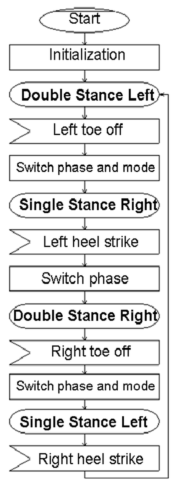
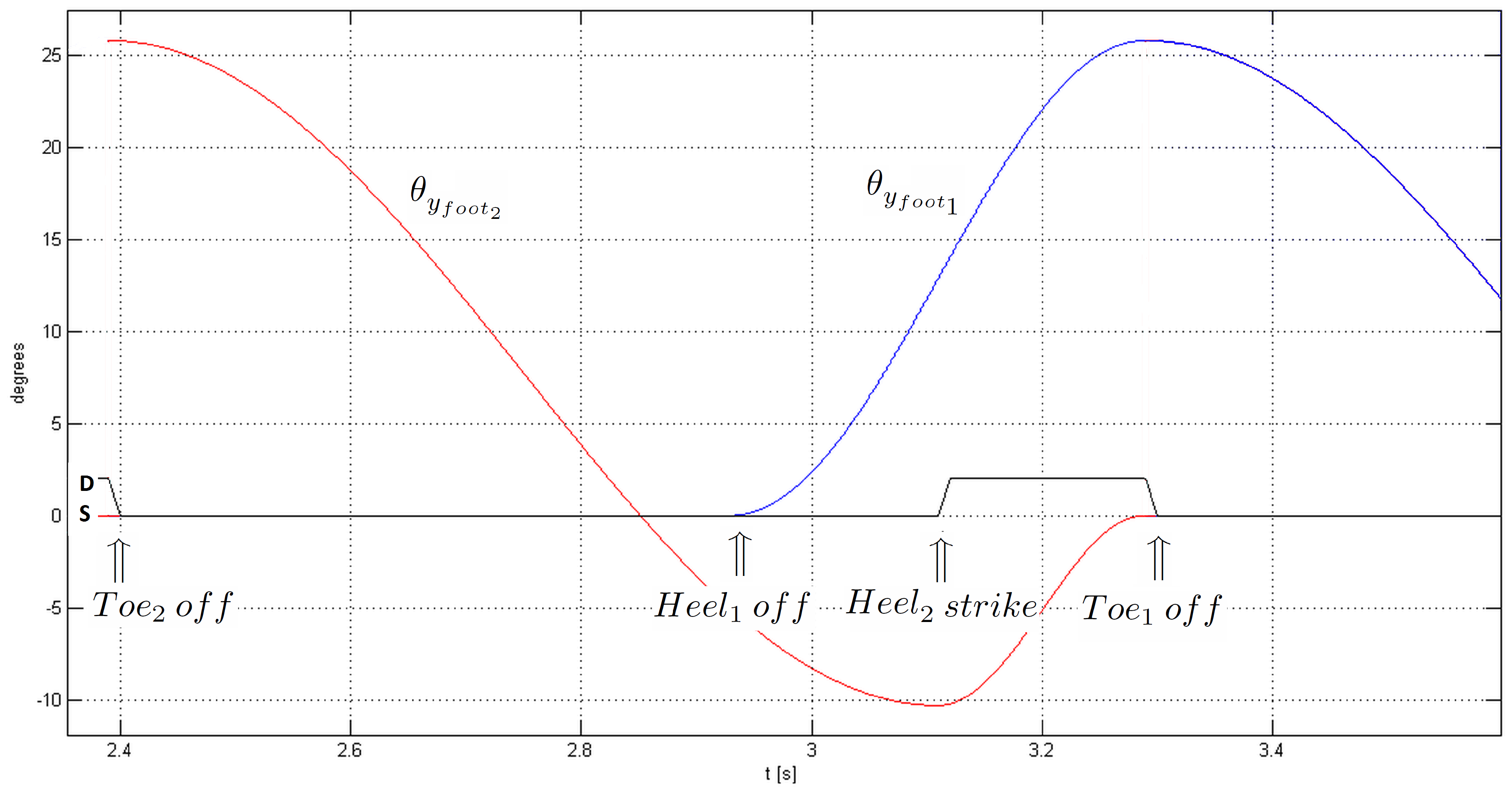
3.4. The Stride in a Gait Cycle

A stride in a gait cycle, when walking, is composed of two main phases (double and single stance) and several sub-phases [18,19,20]. Figure 3 shows an example of one step with the major events.

While the sub-phases defined by the physiologists cannot be adopted directly here, as they don’t refer to different mechanical configurations, the event will be used in the paper.

For simplicity in the presented approach, system is switching between the two main phases only.

Double stance In the double stance model the two feet are hinged to the ground $foo{t}_1$ at $to{e}_1$ and $foo{t}_2$ at $hee{l}_2$. During the stance, starting from the event $Hee{l}_{2}strike$ from the previous single stance, followed by $Foo{t}_{2}flat$ and terminating with $To{e}_{1}off$ (For simplicity here these last two events are set at the same instant.), the weight is transferred from $foo{t}_1$ to $foo{t}_2$.

Single stance In the single stance model the supporting $foo{t}_1$ is hinged at $to{e}_1$. The phase starts with the supporting $foo{t}_1$ $flat$ at the event $To{e}_{2}off$, followed by $Hee{l}_{1}off$ and ending with $Hee{l}_{2}strike$. If during the first sub-phase the posture is controlled by the support of the foot flat on the ground, during the second the active torque on the $to{e}_1$ joint is needed.

Note that there are two symmetrical models for each stance. We define them as $modes$: right (the conventional one of Figure 1 and Figure 2) and left mode. They differ by a parameter that assumes the value $+1$ for the right mode and $-1$ for the left mode, and by exchanging the two sets of limb indexes in the left mode. During the gait, in order to alternate right stance phase and left stance phase, we adopted the following convention: when switching from single to double stance the same mode is maintained, from double to single stance the mode is switched.

4. Building the Simulator

4.1. The Autolev Symbolic Computation

In Autolev the description of holonomic or non-holonomic systems is identical. Along with the definition of the structure of the multichain (bodies, points, segment $COGs$, masses, inertias, kinematical relationships). For the dynamics, input forces/torques, states and output variables have to be specified. States are however divided in positions and velocities, linked by kinematical differential equations:

State 1 the generalized coordinates;

State 2 the generalized speeds;

Kinematical differential equations the relationships between coordinate derivatives and speeds (Equation (6);

Input all forces and torques (comprehensive of those returned by the constraints) with reference, respectively, to the points or bodies of application, to be considered external, hence to be possibly controlled;

Output the desired variables in output, e.g., joint angles and speed, $COG$ and $ZMP$ coordinates, swing foot coordinates, Jacobian matrices, linearizations matrices of the differential equations, reaction forces/torques, matrices of partial derivatives of reaction forces/torques with respect to input control torques, partial velocities, generalized impulse, generalized momentum, etc. In addition, for non-holonomic systems it is required to declare:

• the non-holonomic constraints on the generalized speeds (see Equation (12));
• the selected dependent generalized speeds;
• forces and torques, in the previous declaration, resulting from the constraints, therefore, not to be considered as external input, but internally derived by the simulator.

The Autolev environment interprets the configuration and declarations and generates the dynamical equations and espressions for the output variables (individuals, vectors or matrices as defined), splitting for efficiency in an array of internal variables (called Z) the intermediate results. As output, the source code in C, Fortran or Matlab and an initialization file are returned. Two group of files are then generated, one for each stance.

4.1.1. The Generated Code

The code generated for simulation is composed of the variable declarations, a main program and a set of routines. Among them, a group of service routines are identical for any configuration (reading input parameters and initial conditions, formatting output variables, implementing Runge-Kutta numerical integration), vice versa, three functions are specific of each configuration:

Initialization parameters and state initialization (setting parameters and initial conditions);

State derivative computation a function that computes the state derivative (generalized coordinates and generalized speeds), given the control input, to be called at each phase initializations and at each sampling period during integration by the Runge-Kutta routine in order to update the intermediate expressions, variables and the state;

Output computation a function to calculate at each sampling period any other intermediate expression or variable dependent on the state, state derivative, and input, declared as output in the program. These samples are also saved in a file at the end of the simulation.

For control, a module (the controller) has to be added to the simulation code that sets before each sampling time, the values of forces/torques declared as control input.

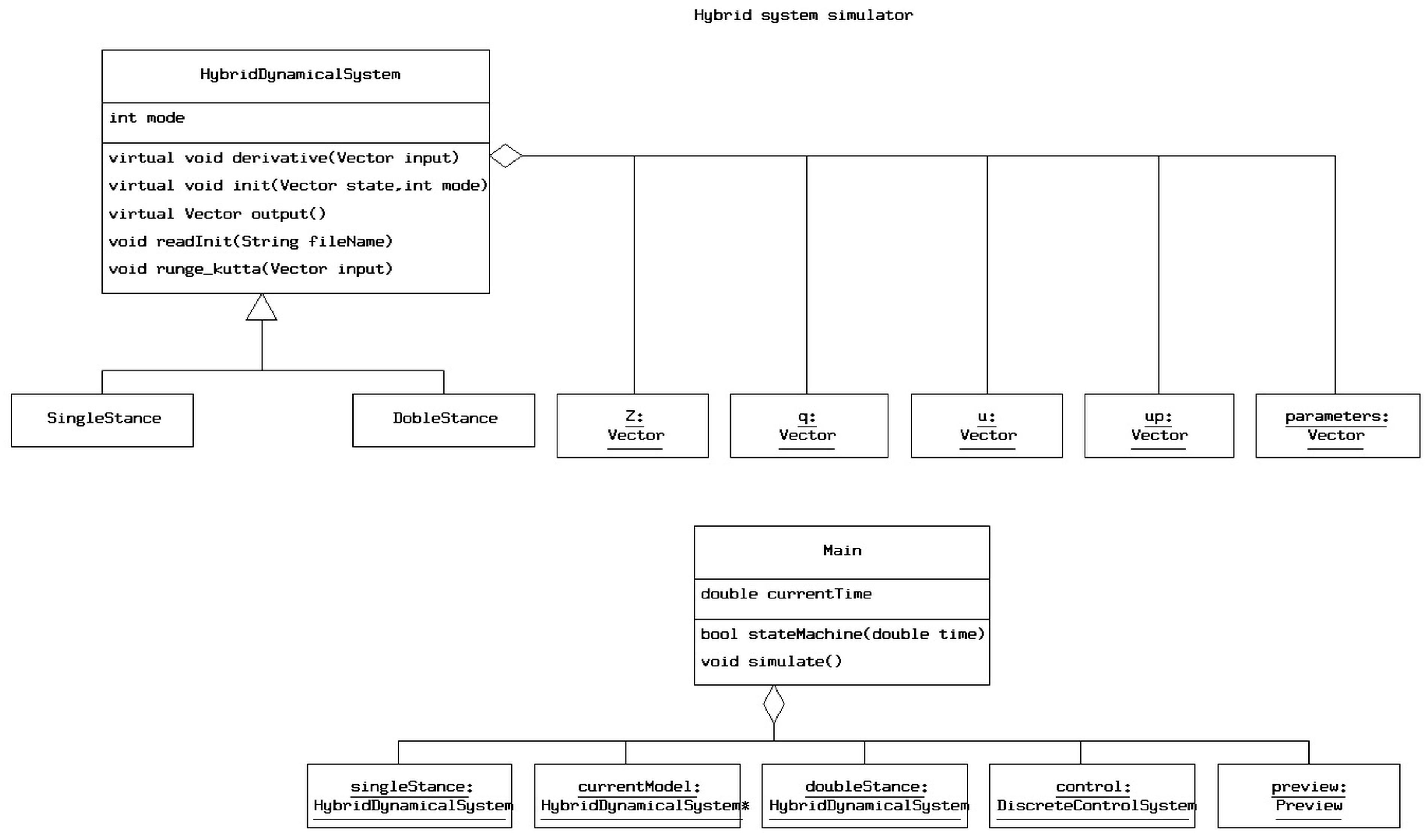
4.2. The Object Oriented Composition of the Program

The C code returned by Autolev, with a few simple modifications, that we automated with a parser, can be embedded in an object oriented programming framework originating one class for each phase of the system, all inheriting from a common base parent, as shown in Figure 4. The base parent contains the declaration of the common variables (intermediate expressions Z, parameters, generalized coordinate, generalized speeds and their derivatives, and the $mode$ variable ($+1,-1$), implements the common service routines, and declares as virtual one protected method for computing the derivative of the state, and two public methods: one for initialization in the right and left mode, and one for returning output variables. Each one of the phase classes implements the three virtual methods.

4.2.1. The Main Class

The main class has as member variables one instance of each phase class (SingleStance, DoubleStance) of the system, a pointer to the $currentModel$, a $Preview$ to generate the reference trajectories, and a $Control$ class to generate the control inputs. It runs the simulation from initial to final instants with two threads: one, event driven ($To{e}_{1}off$, $Hee{l}_{2}strike$), controlling the phases and modes through a state machine, depicted in Figure 5, the other with a given fixed sampling time closing the control loop. Samples of Autolev Code Fragments for building the model and generate the C++ code are presented in Appendix A.

The Preview

The preview generates the nominal reference trajectories of the robot in the Cartesian space, composed by the $COG$ and $COP$ trajectories in the frontal and sagittal planes, the position and angles of the swing foot in single stance, the rotation angles of both feet in double stance.

The Control

The control is a sampled time hybrid dynamical system: at each time period it receives reference and feedback signals and returns the control, updating its state. It switchs configuration at each phase of the model.

5. Conclusions

In this paper, a modelling approach and a computer simulator for biped robotics, outlining the advantages of adopting the Kane’s method to describe the dynamics, has been proposed. The simulator has been developed in Object Oriented programming with the C++ language by exploiting, for the software code of the mathematical expressions, the symbolic dynamic manipulator $Autolev$ that complements the Kane’s method. The Kane’s method together with $Autolev$, with the introduction of intermediary variables to avoid repetions, assure tha maximum efficiency of computation.

As a case study, a 3D standard 12 DOF biped configuration has been considered, however it is clear that the approach can be advantageously applied to different configurations.

Especially attractive is the handling of non-holonomic constraints, when used for rehabilitation, with the possibility to embed in the model different kinds of constraints, as mentioned in Section 2, such as interaction with a chair or a pair of crutches, a thrust, etc. In fact the original motivation of this work has been the development of a lower limb haptic exoskeleton for postural rehabilitation, that is actually being currently built under Italian Government grants, and a sit-to-stand exercise implementation [22].

The object oriented framework adopted to develop the simulator is based on the $G++$ programming environment by SYCO [21].

Examples of controls based on this model can be found in [2] and in part 2 and 3 of this paper.

References

1. Menga, G. Team Isaac: Academic Research Project on Robotic Humanoids. Available online: http://www.isaacrobot.it/ (accessed on 17 March 2016).
2. Menga, G.; Ghirardi, M. Lower Limb Exoskeleton with Postural Equilibrium Enhancement For Rehabilitation Purposes. Internal report DAUIN - Politecnico di Torino. 2015. Available online: https://dl.dropboxusercontent.com/u/26129003/SUBM1.pdf (accessed on 17 March 2016).
3. MSC Software, MSC Adams Multibody Dynamics Simulation. Available online: http://www.mscsoftware.com/Products/CAE-Tools/Adams.aspx (accessed on 17 March 2016).
4. Hurmuzlu, Y.; Genot, F.; Brogliato, B. Modeling, stability and control of biped robots—A general framework. Automatica 2004, 40, 1647–1664. [Google Scholar] [CrossRef]
5. Heemels, W.P.M.H.; Brogliato, B. The complementarity class of hybrid dynamical systems. Eur. J. Control 2003, 9, 322–360. [Google Scholar] [CrossRef]
6. Siciliano, B.; Oussama, K. Springer Handbook of Robotics; Springer: Berlin, Germany; Heidelberg, Germany, 2008. [Google Scholar]
7. Kane, T.R.; Levinson, D.A. Dynamics: Theory and Applications; McGraw-Hill: New York, NY, USA, 1985. [Google Scholar]
8. Gillespie, R.B. Kane’s equations for haptic display of multibody systems. Haptics-e 2003, 3, 144–158. Available online: http://www.haptics-e.org (accessed on 17 March 2016). [Google Scholar]
9. Mitiguy, P. MotionGenesis: Advanced Solutions for Forces, Motion, And Code-Generation. Available online: http://www.motiongenesis.com/ (accessed on 17 March 2016).
10. Azevedo, C.; Espiau, B.; Amblard, B.; Assaiante, C. Bipedal locomotion; toward a unified concept in robotics and neuroscience. Biol. Cybern. 2007, 96, 209–228. [Google Scholar] [CrossRef] [PubMed]
11. Azevedo, C.; Amblard, B.; Espiau, B.; Assaiante, C. A Synthesis of Bipedal Locomotion in Human and Robots; Technical Report; Research Report 5450; INRIA: Sophie Antipolis Cedex, Nice Cedex, France, 2004; Available online: https://hal.inria.fr/inria-00070557 (accessed on 17 March 2016).
12. Wieber, P. Constrained Stability and Parameterized Control. In Biped Walking, Proceedings of the International Symposium on Mathematical Theory of Networks and Systems, Perpignan, France, 19–23 June 2000.
13. Wieber, P. On the Stability of Walking Systems. In Proceedings of the International Workshop on Humanoids and Human Friendly Robotics, Tsukuba, Japan, 11–12 December 2002.
14. Kumar, R.; Handharu, N.; Jungwon, Y.; Gap-soon, K. Hybrid toe and heel joints for biped/humanoid robots for natural gait. In Proceedings of the International Conference on Control, Automation and Systems, Seoul, Korea, 17–20 October 2007.
15. Ezati, M.; Toosi, K.; Khadiv, M.; Moosavian, S. Dynamics modeling of a biped robot with active toe joints. In Proceedings of the 2014 Second RSI/ISM International Conference on Robotics and Mechatronics, Tehran, Iran, 15–17 October 2014.
16. Ezati, M.; Khadiv, M.; Akbar, M.S.A. Optimal gait planning for a biped robot by employing active toe joints and heels. Modares Mech. Eng. 2015, 15, 69–80. [Google Scholar]
17. Bajodah, A.H.; Hodges, D.; Chen, Y. Nonminimal generalized Kane’s impulse-momentum relations. J. Guid. Control Dyn. 2004, 27, 1088–1092. [Google Scholar] [CrossRef]
18. Ounpuu, S. The biomechanics of walking and running. Clin. Sports Med. 1994, 13, 843–863. [Google Scholar] [PubMed]
19. Saunders, J.B.; Inman, V.T.; Eberhardt, H.D. The major determinants in normal and pathological gait. J. Bone Joint Surg. 1953, 35-A, 543–558. [Google Scholar] [PubMed]
20. Patton, J. Normal Gait Part B of Kinesiology. Technical Report. 2002. Available online: http://www.smpp.northwestern.edu/˜jim/kinesiology/partB_GaitMechanics.ppt.pdf (accessed on 17 March 2016).
21. Menga, G. G++ Programming Environment, SYCO. 2008. Available online: www.syco.it (accessed on 17 March 2016).
22. Bahar, B.; Miskon, M.F.; Bakar, N.A.; Shukor, A.Z.; Ali, F. Path generation of sit to stand motion using humanoid robot. Aust. J. Basic Appl. Sci. 2014, 8, 168–182. [Google Scholar]
Figure 1. The robot: frontal plane - joint configuration.
Inventions 01 00006 g001
Figure 2. The robot: sagittal plane—single and double stance.
Inventions 01 00006 g002
Figure 3. behaviour of the θ y f o o t i and the major events during a step.
Inventions 01 00006 g003
Figure 4. The object model of the simulator in UML notation [21].
Inventions 01 00006 g004
Figure 5. The state machine of the simulator in SDL notation [21].
Inventions 01 00006 g005