Analytics of Deep Neural Network-Based Background Subtraction

Abstract

Deep neural network-based (DNN-based) background subtraction has demonstrated excellent performance for moving object detection. The DNN-based background subtraction automatically learns the background features from training images and outperforms conventional background modeling based on handcraft features. However, previous works fail to detail why DNNs work well for change detection. This discussion helps to understand the potential of DNNs in background subtraction and to improve DNNs. In this paper, we observe feature maps in all layers of a DNN used in our investigation directly. The DNN provides feature maps with the same resolution as that of the input image. These feature maps help to analyze DNN behaviors because feature maps and the input image can be simultaneously compared. Furthermore, we analyzed important filters for the detection accuracy by removing specific filters from the trained DNN. From the experiments, we found that the DNN consists of subtraction operations in convolutional layers and thresholding operations in bias layers and scene-specific filters are generated to suppress false positives from dynamic backgrounds. In addition, we discuss the characteristics and issues of the DNN based on our observation.

1. Introduction

Change detection is a key technology in video surveillances. Background subtraction is an effective method for detecting changes in images; it compares an observed image to a background model such as a background image. Foreground segmentation is provided as changes between an observed image with respect to a background model based on only background information. The background contains no changes of interest generated by dynamic backgrounds, such as rippling water, waving trees, and pedestrian shadows. We designed better background features to ignore changes that are not of interest in the dynamic backgrounds. Several researchers have proposed effective background subtraction and background modeling strategies to detect only changes of interest [1].

A background model is designed based on a heuristic approach. The simplest background model uses a background image with no foreground, such as moving objects. This method is incapable of handling dynamic backgrounds such as waving trees and darkening regions. Some authors define backgrounds using statistical methods, such as Gaussian mixture model [2] and kernel density estimation-based modeling [3], to represent dynamic backgrounds. Texture-based features, such as a local binary pattern [4], are often used to adapt to illumination changes. In addition, some features and background models are combined to enhance the robustness to background changes [5,6]. However, these heuristic approaches work well only for scenes containing background features designed by the researchers. Designing perfect background features manually is extremely challenging, because the background changes are caused by several factors, such as shadows from foreground objects, weather changes, and camera jitter. These factors are summarized in the Changedetection.net 2014 (CD2014) dataset [7].

Some researchers have begun using deep neural networks (DNNs) for background subtraction [8,9,10,11,12]. Zhang et al. [8] and Shafiee et al. [9] used high-dimensional features from DNNs for background modeling. Some authors [10,11,12] proposed a background subtraction framework using a convolutional neural network. DNN-based methods automatically discover the background features from training images. DNN-based background subtraction and background modeling outperformed handcraft-based approaches using background features and/or background subtraction strategies designed by researchers. However, the authors rarely mention how and why DNNs work well for background changes. Foreground/background labels are used as ground truth to train DNNs even though handcraft-based approaches do not use foreground information. DNNs may be specific foreground detectors, such as a vehicle detector and a pedestrian detector.

In our previous work [13], we investigated the fundamental behaviors of the DNN based on Braham’s network [10]. Therein, we mainly focused on the first and last layer. In this work, we aimed to analyze DNN behaviors in all layers. Furthermore, we discussed the characteristics and issues of the DNN-based background subtraction as a summary of our experiments. To observe DNN behaviors, we visualized the feature maps in all layers. We modified Braham’s network for analyzing feature maps in the network. Braham’s network is a patch image-based method that provides feature maps with lower resolution than a patch image. The modified network can provide feature maps with the same resolution as a full image used as an input. The modification facilitates the observation of feature maps comparing the full image easily, as illustrated in Figure 1. We investigated feature maps directly and to recognize which filter is important for the detection accuracy. In following sections, we discuss related works. Then, we describe modification of the network and report results of the analysis.

2. Related Work

Background subtraction strategies and background modeling methods are proposed for the computer vision field. The methods detect differences between an observed image and a background image. A primary issue is to distinguish the differences by foregrounds from ones by dynamic backgrounds, such as illumination changes and waving trees. To solve this issue, statistical methods [2,3] and case-based methods [14,15] were proposed to model efficient backgrounds. Robust background features, such as texture-based features [4,16] and frame-wise information [17], are used for background subtraction. However, recent DNNs outperformed the handcraft-based methods in terms of detection accuracy.

Some authors used DNNs for background feature extraction. Donahue et al. [18] investigated that DNNs trained on ImageNet extracts more effective features than handcraft-based features, such as GIST [19] in other visual tasks. Shafiee et al. [9] used high-dimensional features from a DNN trained on the ImageNet dataset [20] for constructing the Gaussian mixture models. Zhang et al. [8] proposed binary features calculated from the features extracted by stacked denoising autoencoder. Braham et al. [21] used a semantic segmentation map generated from PSPNet [22] for modeling foregrounds and backgrounds. They provided better results than handcraft-based features. These methods used handcraft-based background subtraction strategies.

Other authors emulated background subtraction strategies based on DNNs framework [10,11,12,23]. DNNs exhibit excellent performances in segmentation tasks such as semantic segmentation tasks [22,24,25] and foreground segmentation tasks [26]. DNN-based background subtraction methods have different frameworks [22,24,25]. DNNs in [22,24,25] used a single image as an input, whereas the DNN-based background subtraction in [10,11,12,23] used more than two images consisting of observed images and a background image.

Braham and Droogenbroeck [10] proposed a convolutional neural network for background subtraction. They modified the LeNet-5 network [27]. The input of the network consists of two patch images extracted from an observed image and the corresponding background image. The background images are generated from training images in each specific scene by a temporal median filter. The network provided the foreground probability with a central pixel in the patch image. Unlike traditional background subtraction methods, the foreground mask is needed as the supervised signal for training the network. Their foreground segmentation accuracy outperformed that of traditional methods. Babaee et al. [11] trained one network using various image sequences from the CD2014 dataset [7]. The input is the observed patch image and a background patch image. Babaee’s DNN provided foreground probabilities for all the pixels of each patch image unlike [10]. They reported the accuracy of the foreground detection and trained filters. Lim et al. [12] proposed an encoder-decoder-based network that generated a segmentation map from two successive images and a background image. The segmentation map was binarized to obtain a foreground segmentation image. Furthermore, the background image was updated using the foreground segmentation image. In [23], three-dimensional (3D) convolutional neural networks were proposed to detect moving objects. The networks accepted some successive images as inputs. Thus, the 3D convolutional neural networks were designed to focus on temporal changes.

The authors mainly discussed detection accuracies of the DNNs. Very little is known about the behavior of the DNNs for background subtraction in these previous works. Analysis of the DNN-based background subtraction is needed for discussing the characteristics and the issues. Visualization methods for analyzing DNNs are proposed [28,29,30]. The authors visualized features contributing to classification by DNNs. In this study, we observed activation maps similar to their visualization works. Additionally, we focused on roles of layers such as convolution layers and bias layers.

3. Analysis of Background Subtraction Network

3.1. Network Architecture

We modified Braham’s network [10] because of easy analysis of feature maps in all layers. Braham’s network uses a patch image cropped from a full image as an input and provides a foreground probability at a central pixel in the patch image. A feature map resolution in Braham’s network becomes much lower than the full image resolution because Braham’s network uses max-pooling layers with an un-overlapping manner. Understanding the roles of the middle layers by observing the low resolution feature maps is challenging.

Our modified network used a full image as an input and provided a foreground probability image, as illustrated in Figure 1. A feature map generated by our modified network had the same resolution as the full image because the size of the filters in all the max-pooling layers was $3\times 3$ with a $1\times 1$ stride. The feature map resolution was not changed by max-pooling with a $1\times 1$ stride. This modification facilitated our analysis, owing to easy visualization. We observed features at all pixels in an image at the same time, as illustrated in Figure 1. Braham’s network can only provide features of small patch image, and 2D positions $(x,y)$ on the feature map do not correspond to 2D positions on an image. In addition, the implementation was more efficient than in Braham’s network in a testing step because our modified network accepted images as the inputs directly. Braham’s network has to compute foreground probability values of all patch images in each frame in a testing step. For example, when a test image size is $320\times 240$, Braham’s network computes foreground probability $320\times 240=76,800$ times.

As illustrated in Figure 1, every layer in the modified network contains three or four sub-layers (convolution layer, bias layer, activation layer and max-pooling layer). A bias layer adds biases to feature maps after the previous convolution layer convolves feature maps with filters. We used a rectified linear unit (ReLU) in each layer, except the output layer with a sigmoid function as activation functions similar to Braham et al. [10]. The width and height of the filters in all the convolution layers was $5\times 5$ with a $1\times 1$ stride. We used gray-scale images, and the image size was $320\times 240$. Therefore, the input size of the network was $320\times 240\times 2$ because the input was obtained by concatenating an observed image with its background image. In Section 4, we describe the details of our network used in experiments.

3.2. Training Details

We minimized a pixel-wise cross-entropy cost function E and followed the network initialization process of [10].

$$E\left(f\right)=\frac{-1}{NM}\sum _n^N\sum _m^M(t_{n,m}log\left(f\left({\mathbf{x}}_{n,m}\right)\right)+(1-t_{n,m})log(1-f\left({\mathbf{x}}_{n,m}\right))),$$

(1)

where N is mini-batch size, M is the number of pixels in an image, ${\mathbf{x}}_{n,m}$ is m th location in an image of n th mini-batch, $t_{n,m}$ is a supervised signal for ${\mathbf{x}}_{n,m}$ and $f\left({\mathbf{x}}_{n,m}\right)$ is the network output of ${\mathbf{x}}_{n,m}$. $t_{n,m}=1$ and $t_{n,m}=0$ mean foreground class and background class, respectively. The filters in the convolution layers are initialized randomly from a normal distribution $\mathcal{N}(0,0.01)$. When the magnitude of the initial values was greater than 0.2, we re-picked the initial values. We initially set the bias in bias layers to 0.1. We used an RMSProp optimizer [32] with a learning rate of 0.001 over 50,000 iterations. We used a mini-batch size of two. Training images contained more background pixels than foreground pixels. Therefore, at least one image in each mini-batch contained foreground objects for preventing over-fitting for background regions.

3.3. Training Data

The CD2014 dataset [7] includes various background changes such as dynamic background and illumination changes from surveillance cameras. In addition, pixel-wise manually labeled ground truth images are available, which have five types of labels (static, hard shadow, outside region of interest, unknown motion, and motion). We defined the motion label as a foreground label and the other labels as a background label except the outside region of interest label. We excluded the outside region of interest label while computing the cost function E. We divided the original sequence into two sub-sequences for training and testing. Images in the original sequence had the corresponding ground truth images. We used the ground truth images in training sub-sequences as the supervised signals for training our modified network.

We prepared a background image from all the training images in each sequence by using a temporal median filter method as in [10]. However, some background images prepared using the temporal median filter retained foreground objects; thus, we eliminated these sequences from the shadow and dynamic background category used in our experiment. We converted the RGB color images to gray-scale images and resized the images to $320\times 240$. We divided the intensity of gray-scale images by 255 to obtain a normalized intensity between 0 and 1.

3.4. Background Subtraction Process

We concatenated the observed image in the testing step with its background image prepared in the training step. The concatenated image was the input of our modified network. When our modified network generated foreground probability image, we thresholded the foreground probability image for obtaining a foreground segmentation image. We set the threshold parameter to 0.5. However, we did not perform any post-processing.

4. Experiments

First, we investigated whether our modified network extracts scene- and/or object-specific features from training images. Second, we observed the feature maps using seven image sequences from the shadow and dynamic background categories in the CD2014 dataset. We discussed how our modified network classified a dynamic background region into a background class qualitatively. Finally, we quantitatively determined the filters critical for detection performance.

Table 1. Detailed architecture of our network. A convolution filter size is represented as Height × Width × Input Channels × Output Channels. A max-pooling filter size is represented as Height × Width. We exclude the bias and activation layers for readability. 2NN-large has the same number of parameters in convolution filters as 4NN.

Layer	4NN	3NN	2NN	2NN-large
Convolution	$5\times 5\times 2\times 6$	$5\times 5\times 2\times 6$	$5\times 5\times 2\times 6$	$5\times 5\times 2\times 30$
Max-pooling	$3\times 3$	$3\times 3$	$3\times 3$	$3\times 3$
Convolution	$5\times 5\times 6\times 6$	$5\times 5\times 6\times 6$	-	-
Max-pooling	$3\times 3$	$3\times 3$	-	-
Convolution	$5\times 5\times 6\times 6$	-	-	-
Convolution	$5\times 5\times 6\times 1$	$5\times 5\times 6\times 1$	$5\times 5\times 6\times 1$	$5\times 5\times 6\times 30$

presents the architecture used in our experiments.

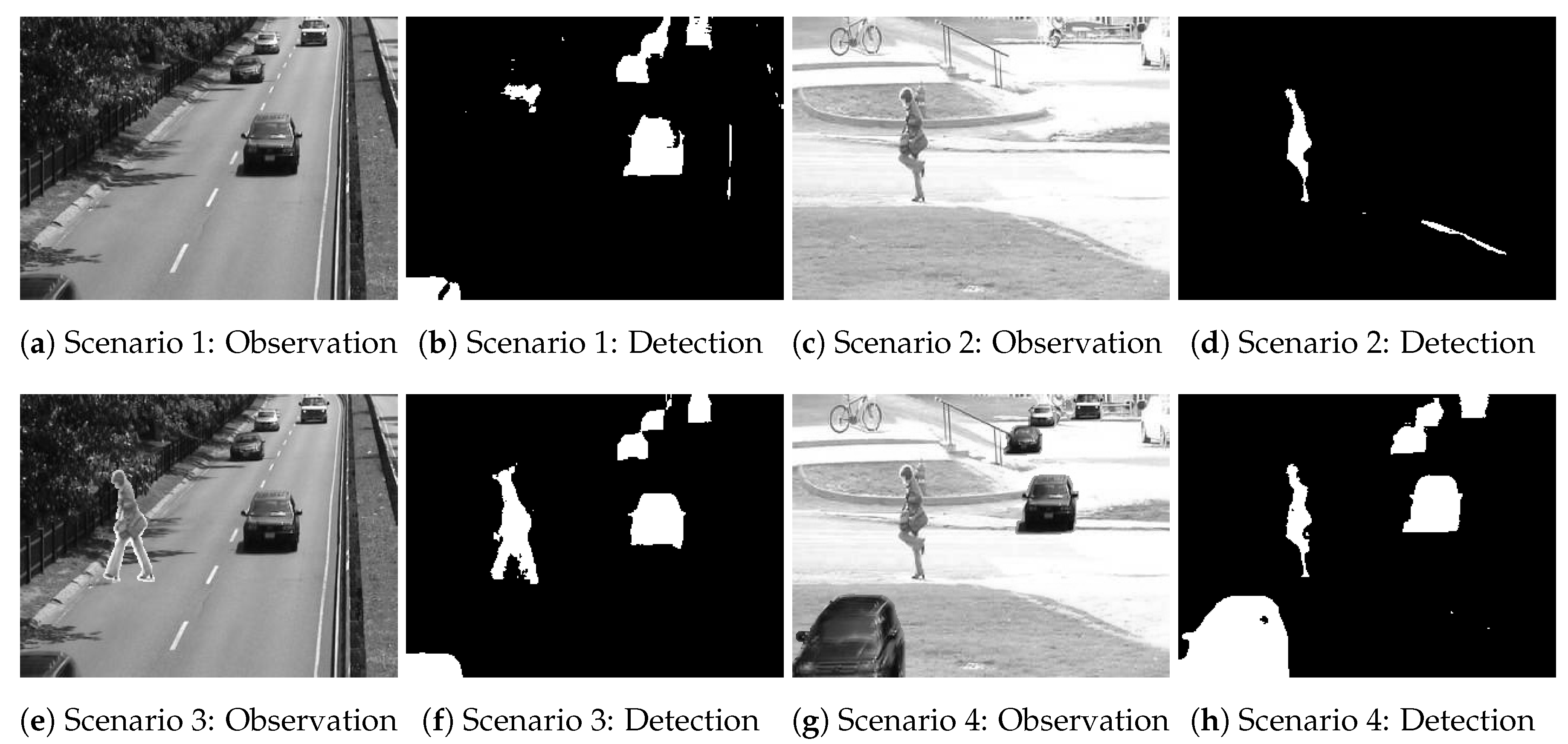
4.1. Experiment 1

We attempted to confirm that our modified network is not an object-specific detector, similar to Braham’s network. We slightly modified Braham’s network as described in Section 3.1. The modification might possibly cause that the network detects specific foregrounds such as cars and people included in the training images. In Table 1, 4NN is used for Experiment 1.

We used two sequences in the CD2014 dataset: highway (HW) and pedestrians (PED). The HW sequence contains vehicles as foreground objects and a road and trees as backgrounds. The PED sequence contains pedestrians as foreground objects and a park as backgrounds. Foreground objects and backgrounds in the HW sequence are completely different from those in the PED sequence.

We consider four scenarios.

Scenario 1

The training sequence is the PED sequence. The testing sequence is the HW sequence.

Scenario 2

The training sequence is the HW sequence. The testing sequence is the PED sequence.

Scenario 3

The training sequence is the HW sequence. The testing sequence is the modified HW sequence.

Scenario 4

The training sequence is the PED sequence. The testing sequence is the modified PED sequence.

Our network did not learn intensity values and shapes of foreground objects appearing in the testing sequences because the PED and HW sequences contain only pedestrians and vehicles as foreground objects, respectively. In Scenarios 1 and 2, background images in the training step were different from those in the testing step. In Scenarios 3 and 4, we superimposed pedestrians and vehicles to the testing sequence of the HW and PED, respectively. The modified HW and the modified PED testing sequence contained pedestrians and vehicles as foreground objects, and the same background image as the original HW and PED sequence. Therefore, in the training steps of only Scenarios 3 and 4, our network learned background information of the testing sequences.

Figure 2 presents the results of all scenarios. In all scenarios, our modified network detected foreground objects even though the foreground objects did not appear in the training sequences. In addition, the network worked in a different background image from that in the training step according to Figure 2b,d. This result indicates that the modified network does not overfit specific foreground objects because the HW and PED sequences do not contain pedestrians and vehicles as the foregrounds, respectively, in the training images.

False positives occurred in some background regions according to the result of Scenarios 1 and 2. In Scenarios 1 and 2, the modified network did not learn background information of the testing sequence. In Scenarios 3 and 4, the modified network correctly classified waving trees and a pedestrian shadow to a background class because of learning background changes from the training images of Scenarios 3 and 4 containing waving tree and pedestrian shadows. Therefore, this implies that the modified network should learn background information of testing sequences for improving detection accuracy.

Figure 3 illustrates visualization of trained six filters in each scenario. The 0th and 1st input channels correspond to a channel for an observed image and a background image, respectively. We observed that the filters detected the differences between the observed image and its background image. In Figure 3, a filter (the 0th output channel in Scenario 4) had higher positive values in the channel for a background image than that for an observed image. Thus, the filter subtracts a background image from an observed image. This observation is in line with that in our previous work [13]. The modified network follows background subtraction similar to Braham’s network.

4.2. Experiment 2

The modified network created subtraction filters in the first layer according to Experiment 1. Thus, the network focused on the differences between an observed and its background image. Dynamic backgrounds such as shadows and waving trees generate such differences, as well as foreground objects. We considered that the differences caused by dynamic backgrounds are canceled in the higher layers. However, observing only the filters is insufficient to understand the role of higher layers. We visualized feature maps in the modified network directly in Experiment 2.

We used seven sequences from the shadow category (bungalows, cubicle, and peopleInShade) and dynamic background category (boats, fall, fountain01, and fountain02) in the CD2014 dataset for training dynamic backgrounds. The seven sequences contained foreground objects in both training and testing images when we divided the original sequence into two sub-sequences for training and testing. The modified network learned each sequence individually. We used four networks described in Table 1 for Experiment 2. 2NN-large had more filters in the first layer than 2NN because of fair comparisons with 4NN. The number of filter parameters in 2NN-large is the same as that in 4NN.

After training the networks, we evaluated the accuracy of foreground detection. All metrics used in our experiments are based on eight metrics of the CD2014 dataset.

Table 2. Performance results of four networks on three sequences of the shadow category in the CD2014 dataset [7]. FPR, FPR-S, FNR, and PWC denote false positive rate, FPR in only shadows, false negative rate, and percentage of wrong classifications, respectively.

	Recall	Specificity	FPR	FNR	PWC	Precision	F-Measure	FPR-S
	bungalows
2NN	0.807	0.997	0.003	0.193	1.342	0.940	0.869	0.155
2NN-large	0.907	0.998	0.002	0.093	0.737	0.957	0.931	0.121
3NN	0.916	0.998	0.002	0.084	0.650	0.964	0.939	0.094
4NN	0.945	0.997	0.003	0.055	0.552	0.955	0.950	0.016
	cubicle
2NN	0.741	0.993	0.007	0.259	1.313	0.752	0.746	0.059
2NN-large	0.877	0.999	0.001	0.123	0.397	0.968	0.920	0.059
3NN	0.880	0.999	0.001	0.120	0.411	0.959	0.918	0.026
4NN	0.908	0.998	0.002	0.092	0.457	0.916	0.912	0.014
	peopleInShade
2NN	0.868	0.996	0.004	0.132	1.121	0.919	0.893	0.460
2NN-large	0.766	1.000	0.000	0.234	1.279	0.994	0.865	0.026
3NN	0.879	0.999	0.001	0.121	0.699	0.989	0.931	0.044
4NN	0.886	1.000	0.000	0.114	0.650	0.992	0.936	0.033

and

Table 3. Performance results of four networks on four sequences of the dynamic background category in the CD2014 dataset [7]. FPR, FPR-S, FNR, and PWC denoted false positive rate, FPR in only shadows, false negative rate, and percentage of wrong classifications, respectively.

	Recall	Specificity	FPR	FNR	PWC	Precision	F-Measure	FPR-S
	boats
2NN	0.484	1.000	0.000	0.516	0.609	0.938	0.639	0.000
2NN-large	0.572	1.000	0.000	0.428	0.514	0.943	0.712	0.000
3NN	0.550	1.000	0.000	0.450	0.534	0.949	0.696	0.000
4NN	0.564	1.000	0.000	0.436	0.491	0.989	0.719	0.000
	fall
2NN	0.877	0.998	0.002	0.123	0.449	0.932	0.904	0.869
2NN-large	0.908	1.000	0.000	0.092	0.262	0.982	0.943	0.711
3NN	0.933	0.999	0.001	0.067	0.243	0.964	0.949	0.753
4NN	0.932	1.000	0.000	0.068	0.187	0.990	0.960	0.499
	fountain01
2NN	0.212	1.000	0.000	0.788	0.095	0.429	0.284	0.000
2NN-large	0.072	1.000	0.000	0.928	0.084	0.877	0.134	0.000
3NN	0.252	1.000	0.000	0.748	0.072	0.805	0.384	0.000
4NN	0.030	1.000	0.000	0.970	0.088	0.578	0.057	0.000
	fountain02
2NN	0.875	0.999	0.001	0.125	0.148	0.398	0.547	0.000
2NN-large	0.872	1.000	0.000	0.128	0.031	0.833	0.852	0.000
3NN	0.789	1.000	0.000	0.211	0.026	0.953	0.863	0.000
4NN	0.923	1.000	0.000	0.077	0.030	0.806	0.861	0.000

report detection accuracies on the seven sequences. Detection accuracies of 2NN were lower than that of the other networks. In particular, 2NN did not work in the peopleInShade sequence that contains pedestrian shadows and illumination changes. The FPR-S of 2NN was 0.460. 4NN, 3NN, and 2NN-large handled dynamic backgrounds by increasing the number of layers or filters in the first layer.

The modified networks demonstrated high detection accuracy except fountain01. Recall values on fountain01 were much lower than those on other sequences. The fountain01 sequence contained one smaller foreground object in the training images. The network failed to generalize the model for background subtraction. In addition, a foreground object size in the test images was nearly 0.7% of the image size. Our modified network did not work well when training and testing images contained very small foreground objects.

We visualized feature maps of our modified network in testing images. Figure 4, Figure 5, Figure 6 and Figure 7 illustrate the examples of the feature map visualization. In these figures, warm and cold colors represent positive and negative values, respectively. In particular, green indicates zero. Figure 4a, Figure 5a,c, Figure 6a, and Figure 7a,c are separated by white lines. The top part contains gray-scale images and heat maps in the observed image and its background image. In order from the top, three or four rows in each part indicate sub-layers (convolution layer, bias layer, activation layer, or max-pooling layer), as shown in Figure 1. In addition, we visualized computational processes in convolution layers by using channel-wise convolutions [31] that calculate convolutions between a feature map and filter every channel, as illustrated in Figure 1. Figure 4b, Figure 5b, Figure 6b, and Figure 7b are separated by white lines, each part corresponding to each convolution layer in order from the top.

According to a feature map of the last convolution layer (C3) in Figure 4a, a shadow (background class) had negative values, whereas a vehicle (foreground class) had positive values. Then, only the vehicle activated through the last sigmoid layer (S3). The observed image was different from the background images in both the shadow and vehicle regions. We distinguished the difference generated by the shadow from the difference generated by the vehicle. To understand how the difference by the shadow was canceled, we focused on the 0th, 4th, and 5th feature maps in the second bias layer (B2). Because of the bias layer, negative values in the shadows changed to positive values. This role of the bias layer is similar to thresholding. According to Figure 4b, Figure 5b, Figure 6b, and Figure 7b, feature maps generated mainly by channel-wise convolution have positive or negative values, thereby indicating that higher layers consist of subtraction operations such as subtraction filters in the first layer. Before the bias layer, feature maps were generated by the second convolution layer that consists of subtraction operations. According our observation, the network performed subtraction and thresholding operations repeatedly to cancel dynamic backgrounds.

Feature maps in Figure 6 were significantly different from those in Figure 4. However, we found discriminative features in the 5th feature map in the 0th bias layer (B0) in Figure 6a. The 5th feature map in B0 was more discriminative than that in the 0th convolution layer (C0). In B0, the vehicle region had positive values and most background regions had negative values. A part of a fountain also had positive values. We distinguished the fountain from the vehicle in the second layer through subtraction and thresholding operations in the convolution and bias layers.

We compared the detection accuracy of the 4NN to the 2NN-large and 3NN when the networks learned each sequence individually. However, feature maps were different among the networks. 2NN-large computed various feature maps generated by subtraction filters in the first layer, then, combined the feature maps to obtain a foreground probability map. Feature maps should discriminative between background and foreground regions in the first layer. We could not judge foregrounds/backgrounds based on their feature maps of the first layer in Figure 5c. Feature maps in the first activation layer activated in both background and foreground regions in Figure 5c. However, 2NN-large detected only a vehicle based on a complex combination of feature maps. We observed that 2NN-large was not robust when a sequence contained more various backgrounds. We trained the four networks using three sequences of the shadow category simultaneously. Thus, the training dataset contained many various backgrounds. In this additional experiment, we trained the networks over 50,000 × 3 iterations because the number of the sequences was three.

Table 4. Average detection accuracies on three sequences of the shadow category in the CD2014 dataset [7]. Networks use the sequences of a shadow category simultaneously. Thus, the dataset complexity increases.FPR, FPR-S, FNR, and PWC denote false positive rate, FPR in only shadows, false negative rate, and percentage of wrong classifications, respectively.

	Recall	Specificity	FPR	FNR	PWC	Precision	F-measure	FPR-S
2NN	0.714	0.992	0.008	0.286	2.079	0.822	0.764	0.526
2NN-large	0.853	0.996	0.004	0.147	1.062	0.918	0.884	0.315
3NN	0.799	0.997	0.003	0.201	1.199	0.941	0.863	0.220
4NN	0.879	0.995	0.005	0.121	1.099	0.893	0.883	0.138

reports the average detection accuracies on the three sequences. An FPR-S value of 4NN was lowest in the other network. The 3NN-large had higher FPR-S value than networks based on the scene-specific training. This indicates that deeper networks can handle dynamic backgrounds when target scenes are more complicated.

In addition, we found difficulty of the network. We observed that a shadow region was not distinguished a vehicle region in the 1st, 2nd, and 3rd feature maps of the last channel-wise convolution (C3) in Figure 4b. Background regions should have negative values in the last channel-wise convolution layer because an activation function in the last layer is a sigmoid function. A sigmoid function returned less than 0.5 when the input was negative. The 1st, 2nd, and 3rd feature maps had positive values in background regions; they may cause false positives. In Figure 4b, the 0th, 4th, and 5th feature maps had negative values in background regions. Therefore, false positives did not occur in this figure. In Figure 7b, the 2nd feature map in the last channel-wise convolution has negative values in a vehicle. Foreground regions should have positive values because an activation function in the last layer is a sigmoid function. These maps may cause false negatives. This visualization assisted in confirming whether the trained network is reasonable.

4.3. Experiment 3

We discussed the network mechanism of foreground decision process qualitatively. However, the results in Experiment 2 did not show the filters in the middle layers that contribute to detection performance. We removed filters to analyze contribution of filters in the middle layer. We focused on filters in the 1st and the 2nd convolution layer of 4NN because of analyzing the middle layers. According to Table 1, the layers have six filters with six input channels. In other words, 72 two-dimensional filters (2D filter) in the layers were available. We used each 2D filter to generate a feature map in a channel-wise convolution. When we removed the 2D filter by replacing all filter values to 0, the feature map computed by the 2D filter was ignored in the foreground detection process of the network. We can analyze the contribution of filters through observing detection accuracies after removing filters. We used trained 4NN and test sequences in Experiment 2.

First, we measured the contribution on detection accuracies in each filter. We selected one of the 72 filters, and then removed it. We evaluated the network again after removing only the filter. Figure 8 represents performance degradation when only single 2D filter is removed from 4NN. F-measure, precision, recall, and specificity are better when the metrics are higher, whereas FNR, FPR, FPR-S, and PWC are better when the metrics are lower. The performance degradation increased when the metrics deteriorated after removing a filter.

Some filters (e.g., L1i4o5 in Figure 8a and L1i5o2 in Figure 8b) significantly decreased almost detection accuracies. These filters are essential components for the foreground detection process by the network. In Figure 8a, when filter L1i5o5 was removed, FPR-S increased greatly and F-measure barely decreased. This result shows that the filter works to classify shadows into backgrounds. In Figure 8b, when filter L2i2o5 was removed, precision decreased in particular. We observed that the false positives occurred in a fountain when removing the filter L2i2o5. Therefore, the filter is critical for canceling changes by dynamic backgrounds. We found that the trained network strongly relied on some filters and generated scene-specific filters to suppress false positives from dynamic backgrounds, such as shadows and fountains. In addition, this result indicated that other filters can be removed without affecting detection accuracies. According to Figure 8, most 2D filters do not affect detection accuracies.

Second, we evaluated performance degradation when removing some filters from the network simultaneously. A filter is removed as priority if the filter contributes marginally to performance degradation. The number of removed filters increases step by step. Before removing a filter, we checked the filter in ascending order of F-measure decreases computed in the previous experiment. When performance degradations on the FPR, FPR-S, and F-measure were lower than a threshold, we removed the filter. FPR, FPR-S, and F-measure were chosen as criteria for thresholding because this experiment focused on false positives generated by dynamic backgrounds. After checking all filters, we increased the threshold if all filters are not removed. We repeated the procedure six times in Experiment 3. We set the threshold values to $\left\{0.05t\right|1\le t\le 6\}$. This filter-removing process cannot obtain optimal combination of removed filters on the best detection accuracies. However, computational complexity to obtain the optimal combination is not polynomial time. Therefore, this removing process adapts the greedy algorithm for relaxing the computational complexity.

Figure 9 shows the changes of detection accuracies by removing filters in the bungalows and fountain02 sequences. Dash lines in Figure 9 represent filters reaching the best F-measure value or removed at last in each iteration. Performance degradations on the FPR, FPR-S, and F-Measure are assured below a threshold in each iteration. According to Figure 9, a part of filters in the trained network handles dynamic backgrounds because performance degradation on the FPR, FPR-S, and F-Measure rarely occurred in the first iteration. A main reason of performance degradation was the increases in false negatives because the removing process focused on keeping accuracies on the FPR, FPR-S, and F-measure. The calculation for F-measure uses precision and recall; thus, false negatives did not increase abruptly.

Table 5. Ratio of removed filters (%). These ratios are calculated when the best F-measure value is marked, or a filter is removed at last in each iteration. N/A occurs when all candidates of removed filters cause performance degradation with more than a threshold parameter.

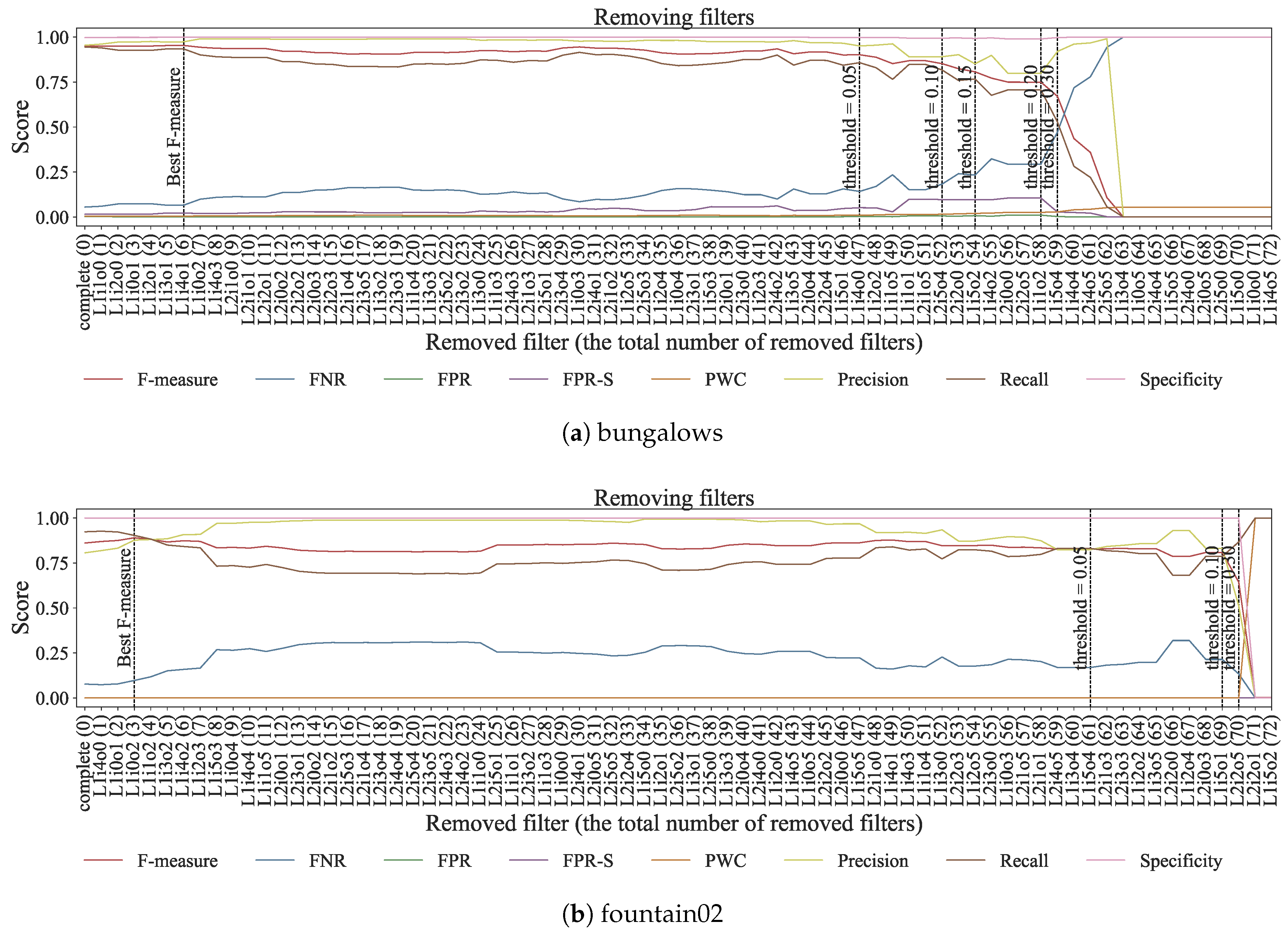
Performance Degrade	0↓(Best)	0.05↓	0.1↓	0.15↓	0.2↓	0.25↓	0.3↓
bungalows	0.0833	0.6528	0.7222	0.7500	0.8056	0.8194	N/A
cubicle	0.1111	0.6528	0.7917	0.8056	0.8194	0.8333	0.8750
peopleInShade	0.1111	0.6111	0.7639	0.8333	0.8750	0.9028	N/A
boats	0.2639	0.4028	0.6250	0.7917	0.8750	0.8889	N/A
fall	0.0417	0.5000	0.5972	0.7222	0.7500	0.7639	0.7778
fountain01	0.1667	0.5833	0.7917	0.8056	N/A	N/A	N/A
fountain02	0.0417	0.8472	0.9583	0.9722	N/A	N/A	N/A

shows the ratio of removed filters in each sequence. As shown in Table 5, the FPR, FPR-S, and F-measure were down 0.05 even when we removed more than 32 filters. In addition, the network marked the best F-measure value when some filters were removed. In other words, some filters contributed to performance degradation. For example, 19 filters in the boats sequence and three in the fountain01 sequence degraded performances. This result suggests further improvement of detection accuracy in the network.

4.4. Discussion

We discussed the characteristics and issues of DNN-based background subtraction, based on the results of Experiments 1, 2, and 3. If the DNN-based network performed scene-specific learning, it worked well because background changes were limited in a specific scene. Therefore, a scene-specific learning enables the network to adapt the filters to background changes in the scene. In Experiment 1, the shadow regions were trained by several filters to reduce false detection of the pedestrian shadows. In Experiment 3, the network could generate filters to adapt for scene-specific background changes such as shadows and fountain. From these findings, we conclude that the DNN-based network provided satisfactory performance when the target was a specific scene; more specifically, the number of types in background changes as limited.

When the DNN-based network trained multiple scenes simultaneously, the detection accuracy decreased. According to the visualization of feature maps in Experiment 2, the DNN consisted of the calculations of subtraction and thresholding. Therefore, the DNN extracts the feature of the difference between observed and background image; then, it detects the foreground regions based on the difference. When it was a scene-specific training, the DNN could generate appropriate filters and their combination strategy to reduce false detection caused by the scene-specific background changes. Meanwhile, when the DNN trained multiple scenes, generating versatile rules shared by multiple scenes was difficult for the network. We tried to train 4NN with more filters in multiple scene training. However, the performance did not reach the one of scene-specific training.

Multiple scenes contain more types of background changes than a specific scene. When the number of types in background changes increased, the network training became difficult. This indicates that acquiring a DNN-based network that can be used for various scenes is challenging. A simplest solution is to generate many scene-specific networks scene by scene and combine them. A good combination strategy should be studied to realize such networks. It is one of our future works.

Finally, we should mention about the relationship between our networks and the other deep background subtraction networks. The other network architectures were different from our network architectures which kept the resolution of the feature maps in all layers. At least, the conclusion which comes from Experiment 1 can be applied to network architectures which reduce the resolution in the deeper layers. We confirmed the fact through our previous experiments reported in the paper in AVSS2017 [13]. With regards to the middle layers in which the resolution is gradually reduced, we guess that the similar characteristics will be observed, because our network architecture was designed to make us easily understand the characteristics by keeping the resolution. In our future work, we are going to investigate whether the conclusions are really applied. Additionally, the other investigations for encoder-decoder based networks are needed because our analysis did not focus on decoder architectures. The decoder increases the resolution of the feature maps from the encoder. Characteristics of the encoder-decoder based network will be much different from ones of our networks.

5. Conclusions

In this study, we investigated how the DNN-based background subtraction works in all layers of the DNN. We modified a patch image-based network to a full image-based network for easy analysis. The modified network provided feature maps with the same resolution as those of a full image. This modification assisted in comparing the feature map with the full image and observe features at all pixels in the full image at once.

We found two behaviors of the DNN used in our experiments. First, the network consists of subtraction operations in convolutional layers and thresholding operations in bias layers. These operations help the network to classify the background changes generated by dynamic backgrounds into the background class. Second, we observed scene-specific filters to cancel background changes from dynamic backgrounds. In addition, a few filters strongly affected detection accuracies.

We discussed the characteristics and issues of the network based on our experiments. The DNN worked well in scene-specific training; however, the DNN performance degraded in multiple scenes training. The multiple scenes training is more challenging for the DNN than the scene-specific training because the multiple scenes contain more types of background changes than a specific scene. In future work, we intend to consider better training strategies to learn multiple scenes simultaneously.

References

- Bouwmans, T. Traditional and recent approaches in background modeling for foreground detection: An overview. Comput. Sci. Rev. 2014, 11, 31–66. [Google Scholar] [CrossRef]
- Stauffer, C.; Grimson, W.E.L. Adaptive background mixture models for real-time tracking. In Proceedings of the 1999 IEEE Computer Society Conference on Computer Vision and Pattern Recognition, Fort Collins, CO, USA, 23–25 June 1999; Volume 2. [Google Scholar]
- Elgammal, A.; Harwood, D.; Davis, L. Non-parametric model for background subtraction. In Computer Vision-ECCV 2000; Springer: Berlin, Germany, 2000; pp. 751–767. [Google Scholar]
- Heikkilä, M.; Pietikäinen, M.; Heikkilä, J. A texture-based method for detecting moving objects. In Proceedings of the British Machine Vision Conference (BMVC), Kingston, UK, 7–9 September 2004; pp. 1–10. [Google Scholar]
- Yoshinaga, S.; Shimada, A.; Nagahara, H.; Taniguchi, R. Statistical Local Difference Pattern for Background Modeling. IPSJ Trans. Comput. Vis. Appl. 2011, 3, 198–210. [Google Scholar] [CrossRef]
- St-Charles, P.L.; Bilodeau, G.A.; Bergevin, R. Flexible background subtraction with self-balanced local sensitivity. In Proceedings of the IEEE Conference on Computer Vision and Pattern Recognition Workshops, Columbus, OH, USA, 23–28 June 2014; pp. 408–413. [Google Scholar]
- Wang, Y.; Jodoin, P.M.; Porikli, F.; Konrad, J.; Benezeth, Y.; Ishwar, P. CDnet 2014: An expanded change detection benchmark dataset. In Proceedings of the 2014 IEEE Conference on Computer Vision and Pattern Recognition Workshops (CVPRW), Columbus, OH, USA, 23–28 June 2014; pp. 393–400. [Google Scholar]
- Zhang, Y.; Li, X.; Zhang, Z.; Wu, F.; Zhao, L. Deep learning driven blockwise moving object detection with binary scene modeling. Neurocomputing 2015, 168, 454–463. [Google Scholar] [CrossRef]
- Javad Shafiee, M.; Siva, P.; Fieguth, P.; Wong, A. Embedded motion detection via neural response mixture background modeling. In Proceedings of the IEEE Conference on Computer Vision and Pattern Recognition Workshops, Las Vegas, NV, USA, 26 June–1 July 2016; pp. 19–26. [Google Scholar]
- Braham, M.; Van Droogenbroeck, M. Deep background subtraction with scene-specific convolutional neural networks. In Proceedings of the 2016 International Conference on Systems, Signals and Image Processing (IWSSIP), Bratislava, Slovakia, 23–25 May 2016; pp. 1–4. [Google Scholar]
- Babaee, M.; Dinh, D.T.; Rigoll, G. A deep convolutional neural network for video sequence background subtraction. Pattern Recognit. 2018, 76, 635–649. [Google Scholar] [CrossRef]
- Lim, K.; Jang, W.D.; Kim, C.S. Background subtraction using encoder-decoder structured convolutional neural network. In Proceedings of the 2017 14th IEEE International Conference on Advanced Video and Signal Based Surveillance (AVSS), Lecce, Italy, 29 August–1 September 2017; pp. 1–6. [Google Scholar]
- Minematsu, T.; Shimada, A.; Taniguchi, R.-i. Analytics of deep neural network in change detection. In Proceedings of the 2017 14th IEEE International Conference on Advanced Video and Signal Based Surveillance (AVSS), Lecce, Italy, 29 August–1 September 2017; pp. 1–6. [Google Scholar]
- Barnich, O.; Van Droogenbroeck, M. ViBe: A powerful random technique to estimate the background in video sequences. In Proceedings of the IEEE International Conference on Acoustics, Speech and Signal Processing (ICASSP 2009), Taipei, Taiwan, 19–24 April 2009; pp. 945–948. [Google Scholar]
- Kim, K.; Chalidabhongse, T.H.; Harwood, D.; Davis, L. Real-time foreground–background segmentation using codebook model. Real-Time Imaging 2005, 11, 172–185. [Google Scholar] [CrossRef]
- Jain, V.; Kimia, B.B.; Mundy, J.L. Background modeling based on subpixel edges. In Proceedings of the IEEE International Conference on Image Processing (ICIP 2007), San Antonio, TX, USA, 16 September–19 October 2007; Volume 6, p. VI-321. [Google Scholar]
- Candès, E.J.; Li, X.; Ma, Y.; Wright, J. Robust principal component analysis? J. ACM (JACM) 2011, 58, 11. [Google Scholar] [CrossRef]
- Donahue, J.; Jia, Y.; Vinyals, O.; Hoffman, J.; Zhang, N.; Tzeng, E.; Darrell, T. DeCAF: A Deep Convolutional Activation Feature for Generic Visual Recognition. In Proceedings of the 31st International Conference on Machine Learning (ICML 2014), Beijing, China, 21–26 June 2014. [Google Scholar]
- Oliva, A.; Torralba, A. Modeling the shape of the scene: A holistic representation of the spatial envelope. Int. J. Comput. Vis. 2001, 42, 145–175. [Google Scholar] [CrossRef]
- Deng, J.; Dong, W.; Socher, R.; Li, L.J.; Li, K.; Li, F.-F. Imagenet: A large-scale hierarchical image database. In Proceedings of the IEEE Conference on Computer Vision and Pattern Recognition (CVPR 2009), Miami, FL, USA, 20–25 June 2009; pp. 248–255. [Google Scholar]
- Braham, M.; Piérard, S.; Van Droogenbroeck, M. Semantic background subtraction. In Proceedings of the 2017 IEEE International Conference on Image Processing (ICIP), Beijing, China, 17–20 September 2017; pp. 4552–4556. [Google Scholar]
- Zhao, H.; Shi, J.; Qi, X.; Wang, X.; Jia, J. Pyramid scene parsing network. In Proceedings of the 2017 IEEE Conference on Computer Vision and Pattern Recognition (CVPR), Honolulu, HI, USA, 21–26 July 2017; pp. 2881–2890. [Google Scholar]
- Sakkos, D.; Liu, H.; Han, J.; Shao, L. End-to-end video background subtraction with 3d convolutional neural networks. Multimedia Tools Appl. 2017. [Google Scholar] [CrossRef]
- Long, J.; Shelhamer, E.; Darrell, T. Fully convolutional networks for semantic segmentation. In Proceedings of the IEEE Conference on Computer Vision and Pattern Recognition, Boston, MA, USA, 7–12 June 2015; pp. 3431–3440. [Google Scholar]
- Noh, H.; Hong, S.; Han, B. Learning deconvolution network for semantic segmentation. In Proceedings of the IEEE International Conference on Computer Vision (ICCV), Santiago, Chile, 13–16 December 2015; pp. 1520–1528. [Google Scholar]
- Wang, Y.; Luo, Z.; Jodoin, P.M. Interactive deep learning method for segmenting moving objects. Pattern Recognit. Lett. 2017, 96, 66–75. [Google Scholar] [CrossRef]
- Lecun, Y.; Bottou, L.; Bengio, Y.; Haffner, P. Gradient-based learning applied to document recognition. Proc. IEEE 1998, 86, 2278–2324. [Google Scholar] [CrossRef]
- Zeiler, M.D.; Fergus, R. Visualizing and understanding convolutional networks. In European Conference on Computer Vision; Springer: Berlin, Germany, 2014; pp. 818–833. [Google Scholar]
- Mahendran, A.; Vedaldi, A. Understanding deep image representations by inverting them. In Proceedings of the 2015 IEEE Conference on Computer Vision and Pattern Recognition (CVPR), Boston, MA, USA, 7–12 June 2015; pp. 5188–5196. [Google Scholar]
- Binder, A.; Bach, S.; Montavon, G.; Müller, K.R.; Samek, W. Layer-wise relevance propagation for deep neural network architectures. In Information Science and Applications (ICISA) 2016; Springer: Berlin, Germany, 2016; pp. 913–922. [Google Scholar]
- Chollet, F. Xception: Deep Learning With Depthwise Separable Convolutions. In Proceedings of the IEEE Conference on Computer Vision and Pattern Recognition, Honolulu, HI, USA, 21–26 July 2017; pp. 1251–1258. [Google Scholar]
- Hinton, G.; Srivastava, N.; Swersky, K. Neural Networks for Machine Learning Lecture 6a Overview of Mini-Batch Gradient Descent. Available online: https://www.cs.toronto.edu/~tijmen/csc321/slides/lecture_slides_lec6.pdf (accessed on 14 May 2018).