Optimization Based Evaluation of Grating Interferometric Phase Stepping Series and Analysis of Mechanical Setup Instabilities


1
Lehrstuhl für Röntgenmikroskopie, Universität Würzburg, Josef-Martin-Weg 63, 97074 Würzburg, Germany
2
Fraunhofer EZRT, NCTS Group Würzburg, Josef-Martin-Weg 63, 97074 Würzburg, Germany
*
Author to whom correspondence should be addressed.
J. Imaging 2018, 4(6), 77; https://doi.org/10.3390/jimaging4060077
Submission received: 30 April 2018
/
Revised: 30 May 2018
/
Accepted: 4 June 2018
/
Published: 7 June 2018
(This article belongs to the Special Issue Phase-Contrast and Dark-Field Imaging)
Abstract
:The diffraction contrast modalities accessible by X-ray grating interferometers are not imaged directly but have to be inferred from sine-like signal variations occurring in a series of images acquired at varying relative positions of the interferometer’s gratings. The absolute spatial translations involved in the acquisition of these phase stepping series usually lie in the range of only a few hundred nanometers, wherefore positioning errors as small as 10 nm will already translate into signal uncertainties of 1–10% in the final images if not accounted for. Classically, the relative grating positions in the phase stepping series are considered input parameters to the analysis and are, for the Fast Fourier Transform that is typically employed, required to be equidistantly distributed over multiples of the gratings’ period. In the following, a fast converging optimization scheme is presented simultaneously determining the phase stepping curves’ parameters as well as the actually performed motions of the stepped grating, including also erroneous rotational motions which are commonly neglected. While the correction of solely the translational errors along the stepping direction is found to be sufficient with regard to the reduction of image artifacts, the possibility to also detect minute rotations about all axes proves to be a valuable tool for system calibration and monitoring. The simplicity of the provided algorithm, in particular when only considering translational errors, makes it well suitable as a standard evaluation procedure also for large image series.
1. Introduction
X-ray grating interferometry [1,2] facilitates access to new contrast modalities in laboratory X-ray imaging setups and has by now been implemented by many research groups after the seminal publication by Pfeiffer et al. in 2006 [3]. The additional information on X-ray refraction (“differential phase contrast”) and ultra small angle scattering (“darkfield contrast”) properties of a sample that can be obtained promises both increased sensitivity to subtle material variations as well as insights into the samples’ substructure below the spatial resolution of the acquired images.
In contrast to classic X-ray imaging, the absorption, differential phase and darkfield contrasts are not imaged directly but are encoded in sinusoidal intensity variations arising at each detector pixel when shifting the interferometer’s gratings relative to each other perpendicular to the beam path and the grating bars. A crucial step in the generation of respective absorption, phase and darkfield images therefore is the analysis of the commonly acquired phase stepping series, which is the subject of the present article. Respective examples are shown in Figure 1 and Figure 2.
In principle, the images within such phase stepping series are sampled at about 5–10 different relative grating positions equidistantly distributed over multiples of the gratings’ period such that the expected sinusoids for each detector pixel may be characterized by standard Fourier decomposition [1,2,3]. The zeroth order term represents the mean transmitted intensity (as in classic X-ray imaging), while the first order terms encode phase shift and amplitude of the sinusoid. The ratio of amplitude and mean (generally referred to as “visibility”) is here related to scattering and provides the darkfield contrast. Higher order terms correspond to deviations from the sinusoid model mainly due to the actual grating profiles and are usually not considered.
Given typical grating periods in the range of 2–10 micrometers, the actually performed spatial translations lie in the range of 200–2000 nanometers. Particular for the smaller gratings, positioning errors as small as 10–20 nm imply relative phase errors in the range of 5–10 percent, causing uncertainties in the derived quantities in the same order of magnitude. The propagation of noise within the sampling positions onto the extracted signals has, e.g., been studied by Revol et al. [4], and first results for the determination of the actual sampling positions from the available image series were shown by Seifert et al. [5] using methods by Vargas et al. [6] from the context of visible light interferometry based on a decomposition of the images into three basis images (to be found by means of principal component analysis and subsequent optimization) corresponding to the transmission image and the amplitude modulated sine and cosine of the phase image. Kaeppler et al. [7] optimized the phase stepping positions by means of minimizing an objective function penalizing variations within the visibility and differential phase images that arise from phase stepping errors. For the case of simultaneous grating stepping and object rotation, von Teuffenbach et al. [8] recently reported the inference of stepping errors as part of a maximum likelihood tomographic reconstruction procedure proposed by Ritter et al. [9]. Finally, the authors just became aware of the parallel work by De Marco et al. [10] who investigated the origination of the particular image artifacts caused by phase stepping jitter in order to derive a postprocessing artifact reduction technique.
Especially with regard to the quantitative analysis of darkfield signals [11,12,13], the reduction or elimination of stepping jitter induced errors is highly desirable. This also applies to the directional darkfield [14,15] and anisotropic darkfield tomography techniques [16,17,18,19,20,21], which rely on the comparability of multiple darkfield images to relate signal variations to the anisotropy and orientation of scatterers. As the tomographic methods furthermore require large amounts (–) of projections, phase stepping series processing efficiency is also an issue. With regard to system calibration and monitoring, the inference of the actual stepping motions from the phase stepping series is of interest.
The present article proposes a simple iterative optimization algorithm both for the fitting of irregularly sampled sinusoids and in particular for the determination of the actual sampling positions. The use of only basic mathematical operations eases straightforward implementations on arbitrary platforms. Besides uncertainties in the lateral stepping motion, the remaining mechanical degrees of freedom (magnification/expansion and rotations) are also considered. The proposed techniques will be demonstrated on a typical data set.
2. Methods
The task of sinusoid fitting with imprecisely known sampling locations will be partitioned into two separate optimization problems considering either only the sinusoid parameters or only the sampling positions while temporarily fixing the respective other set of parameters. Alternating both optimization tasks will minimize the joint objective function in few iterations. The technique is further extended to an objective function considering spatially varying sampling positions to also model (erroneous) relative grating rotations and magnifications.
2.1. Sinusoid Fitting
The sinusoid is defined as a function of phase parameterized by a constant offset o, an amplitude a and a phase offset :
For the purpose of fitting the sinusoid model to given data samples, the equivalent representation as a linear combination of trigonometric basis functions (i.e., as a first order Fourier series) will be more convenient:
parameterized by the constant offset o and two auxiliary amplitudes and with the following identities:
The parameters o, , and of the recast sinusoid model corresponding to the least squares fit to given data samples enumerated by i may be determined by means of the following iterative scheme (introducing the superscript iteration index k):
with the factors of and accounting for the normalization of the respective basis functions and N being the amount of samples enumerated by i. The intermediate variables denote the respective ordinate values of the sinusoid model for iteration k and abcissas . The differences thus correspond to the residuals at iteration k. The scheme reduces to classic Fourier analysis for the case of the abscissas being equidistantly distributed over multiples of and converges within the first iteration in that case. As the incremental updates to , and are proportional to the respective derivatives of the error , the fixpoint of the iteration will be the least squares fit also in all other cases.
For a stopping criterion, the relative error reduction
may be tracked. It is typically found to fall below 0.1% within 10–20 iterations given only slightly noisy data (noise sigma three orders of magnitude smaller than sinusoid amplitude) and within less than 10 iterations for most practical cases. For the special case of equidistributed on multiples of , it will immediately drop to 0 after the first iteration. In practice, a fixed amount of iterations in the range of five to fifteen will therefore be adequate as stopping criterion as well.
2.2. Phase Step Optimization
An underlying assumption of the previously described least squares fitting procedure is the certainty of the abscissas, i.e., the set of phases at which the ordinates have been sampled. As the sampling positions are themselves subject to experimental uncertainties (arising from the mechanical precision of the involved actuators), a further optimization step will be introduced that minimizes the least squares error of the sinusoid fit over deviations from the intended sampling positions . These deviations are expected to be smaller than the typical stepping increment . While this procedure obviously results in overfitting when considering only a single phase stepping curve (PSC), it becomes a well-defined error minimization problem when regarding large sets of PSCs sharing the same actual sampling positions . In other words, an approach to the minimization problem
shall be considered, with j indexing phase stepping curves captured by different detector pixels at identical stepping positions .
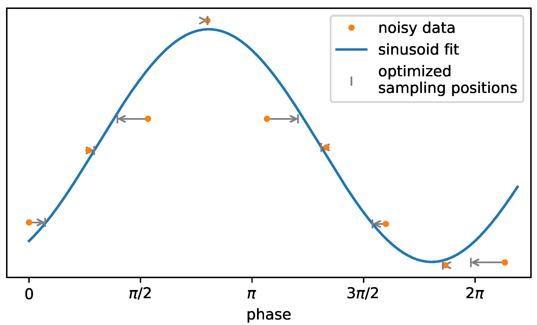
To derive an optimization procedure for the sampling positions, first the fictive case of a perfectly sinusoid PSC with negligible statistical error on the ordinate (the sampled values) shall be considered. Ignoring for now the fact that least squares fits commonly assume only the ordinates to be affected by noise, a least squares fit shall be used to preliminarily determine the parameters of the sinusoid described by the observed data. Assuming then that inconsistencies of the observed data with the model are due to errors on the sampling locations, deviations from their intended positions are given by the data points’ lateral distances from the sinusoid curve (cf. Figure 3). Finally, the actual systematic deviations of the sampling locations can be found by averaging over the respective results for a large set of PSCs sampled simultaneously. This information can be fed back into the original sinusoid fit, which then again allows the refinement of the current estimate of the true sampling positions, finally resulting in an iterative procedure alternatingly optimizing the sinusoid parameters and the actual sampling locations (cf. Algorithm 1).
| Algorithm 1 Least squares optimization of shared abscissa values for simultaneous sinusoid fits to ordinate samples belonging to independent curves j sampled at identical positions . This represents a special case of Algorithm 2 with spatially invariant sampling phases. The relaxation parameter may be chosen <1 if damping of the updates to is desired. For the intermediate argmin operations, see Equations (2)–(5). |
|
| Algorithm 2 Simultaneous least squares optimization of abscissa values and sinusoid fits to ordinate samples belonging to independent curves j sampled at positions with being a slowly varying polynomial with respect to the spatial coordinates and accounting for the expected effects due to translations, magnification and rotations of an interferometer’s gratings. The procedure reduces to Algorithm 1 when considering only the zeroth order term of . |
|
2.2.1. Determination of Individual Phase Deviations
Starting with an initial sinusoid fit
to given data samples , the residual sum of squares shall be minimized over deviations to the abscissas while keeping the sinusoid model parameters o, a and fixed:
For reasons of better readability, the detector pixel index (or equivalently PSC index) j of the sinusoid parameters o, a, and the data samples has been omitted here and is explicitly added again to the final results at the end of this subsection.
Equation (8) is solved when the derivative of the objective function with respect to vanishes:
where the last step is a first order Taylor expansion with respect to . This directly leads to the following expression for :
where the earlier condition is approximated to be satisfied when . The restriction to cases with can be intuitively understood when recalling that implies a maximum or minimum of the sinusoid and means that it is constant ( independent), in both of which cases there is no sensible choice for . The constraint on the result, , can simply be taken into account by means of a limiting function parameterized by a maximal absolute value such as
which converges to the identity function for and is bounded at . The choice of m in this case depends on the validity range of the linear approximation of with respect to about , which obviously depends on the magnitude of the curvature of the sinusoid at this point, as illustrated in Figure 4. This may be accounted for by introducing a suitable dependence to m denoted by the respective argument:
reaches its largest value at (where is actually linear) and smoothly drops to 0 for , in which case both the sine and its curvature are extremal and shall and will be limited to 0. The upper bound for and thus for the choice of is defined by the range of values over which is actually invertible (cf. Figure 4). The sine function is locally invertible over intervals of with n being an integer number and denoting the argument (). For the determination of it is sufficient to consider the case :
For , the linear approximation used in Equation (9) deviates by up to . The deviation is limited to or for and , respectively.
Combining the above results and reintroducing the detector pixel index j, the following expression for pixel (j) and phase step (i) wise phase stepping deviations reducing (and, for sufficiently small , minimizing) the error can be given, choosing :
Figure 3 shows an example of this approximate least squares solution to .
2.2.2. Noise Weighted Average of Phase Deviations
Now that an expression has been derived for the deviations optimizing the abscissa values for individual PSCs indexed by j given previous sinusoid fits, the respective results for all PSCs sharing the same sampling locations may be averaged, such that the mean deviations essentially correspond to the actual systematic phase stepping errors (whereas statistical noise will mostly cancel out):
using weights factoring in the relative certainty and relevance of the individual . An appropriate choiceis
where weights the slope dependent error propagation from noisy measurements to based on the derivative of the sinusoid model at phase step i and weights the contribution of a particular PSC j to the accumulated error. These considerations leadto
where the last step uses the relation for arbitrary real-valued arguments x and m and factors .
Finally, the above derivations can be combined to an iterative optimization algorithm reducing the accumulated least square error of multiple sinusoid fits (indexed by j) to data points over shared abscissa values as defined by Equation (6). A pseudo code representation is given in Algorithm 1, further introducing the relaxation parameter that may be chosen <1 in order to damp the adaptions to if desired. The intermediate sinusoid fits may be accomplished using the iterative algorithm described in the previous section.
2.2.3. Inhomogeneous Sampling Phase Deviations
Up to now, it has been assumed that deviations from the intended phase stepping positions are due to purely translational uncertainties in the relative motion of the involved gratings, resulting in offsets of the actual from the intended sampling phases that are homogeneous throughout the whole detection area. When also considering relative grating period changes (e.g., due to either thermal expansion or motion induced changes in magnification) and rotary motions of the interferometer’s gratings relative to each other (e.g., due to backlashes within the mechanical actuators), the effective sampling phases at each phase step may exhibit gradients over the detection area. Given the small grating periods (micrometer scale) compared to the total extents of the gratings (centimeter scale), both tilts in the sub-microrad range and relative period changes in the range of will already manifest themselves in observable gradients.
The corresponding optimization problem regarding gradients is, analog to Equation (6), given by:
where the spatial dependence of the phase deviations has been accounted for by a functional dependence on the detector pixel index j. Given the expected gradients (as illustrated in Figure 5), the spatially varying phase deviations have the following form:
with the coefficients , , and quantifying the respective gradients in horizontal and vertical direction as well as the mixed term and the curvature in horizontal direction, and h and v being spatial detector pixel indices related to the linear pixel index j through the amount of pixels within one detector row:
The constant offsets and characterize the detector center.
The optimization of the extended objective function in Equation (18) can be performed analog to that of Equation (6) with the only difference lying in the evaluation of the spatial phase difference maps defined by Equation (14) (an example of which is shown in Figure 6). The weighted average derived in the previous section to determine the homogeneous offset can be extended to a generalized linear least squares fit of the model defined by Equation (19) to the local estimates (Equation (14), Figure 6), also taking the weights defined by Equation (16) into account. Said procedure is stated more formally in Algorithm 2.
Basic geometric considerations neglecting higher order interrelations of the considered effects (e.g., rotation and effective period change) result in the following relations between the observable parameters , , , and relative translatory and rotatory motions of the interferometer’s gratings. To relate various magnification changes to spatial motions based on the intercept theorem, an assumption has to be made as to which of the gratings actually moved. Here, the grating that is mounted on the linear phase stepping actuator is assumed to be the cause of all relative motions of both gratings also including tilts and rotations. The “source–grating distance” in the following equations will thus refer to the stepped grating.
quantifies the translational error analog to Section 2.2.2. In contrast to the previous section, the present model distinguishes between homogeneous phase deviations induced by translation and the mean component induced by the term in the case of non-vanishing curvature of the spatial phase deviation.
The vertical gradient parameter is related to a relative rotation of both gratings about the optical axis:
where the “effective grating period” refers to the projected period length at the location of the detector, which should be identical for both interferometer gratings (not considering the optional additional coherence grating close to the X-ray source).
The horizontal gradient parameter is related to a relative mismatch in effective grating periods of the gratings either due to relative distance changes along the optical axis or due to actual expansions (e.g., thermally induced):
When assuming relative grating period mismatches to be caused by changes in magnification due to translations of one of the gratings along the optical axis, the following relation applies to first order:
The change of the horizontal gradient throughout the vertical direction corresponds to a relative change in magnification from top to bottom, e.g., due to a tilt of one of the gratings about the horizontal axis. Using the above relation between magnification changes and spatial displacements, the tilt about the horizontal axis is related to approximately by
A non-vanishing curvature arises in the case of a rotary motion about the vertical axis (slant) and is analogously related to the slant angle to first order by
2.3. Experimental Setup
The interferometer used to demonstrate the described analysis techniques consists of a set of three gratings (coherence grating G0, phase grating G1 and absorption grating G2) manufactured by microworks GmbH (Karlsruhe, Germany) for a design energy of 54keV and mounted in an in house cone beam micro-CT setup comprising a commercial microfocus X-ray source operated at 80 kV acceleration voltage as well as a commercial flat panel detector with a pixel pitch of 74.8 µm. The grating periods are 4.8 µm (G0), 2.4 µm (G1) and 4.8 µm (G2), and the gratings are placed at 100 cm, 125 cm and 150 cm distance from the X-ray source, respectively. The field of view is limited by the diameter of G2 of approximately 10 cm. The G1 grating is mounted on a piezo driven linear actuator responsible for the phase stepping. The detector is placed right behind the absorption grating in about 155 cm distance from the source. Images are averaged over 10 exposures of 0.5 s each and are cropped to a region of 850 × 850 px corresponding to an area of 6.4 × 6.4 cm on the detector. A piece of plastic hose of 2 cm diameter placed about 143 cm distance from the source serves as the sample object.
3. Experiment and Results
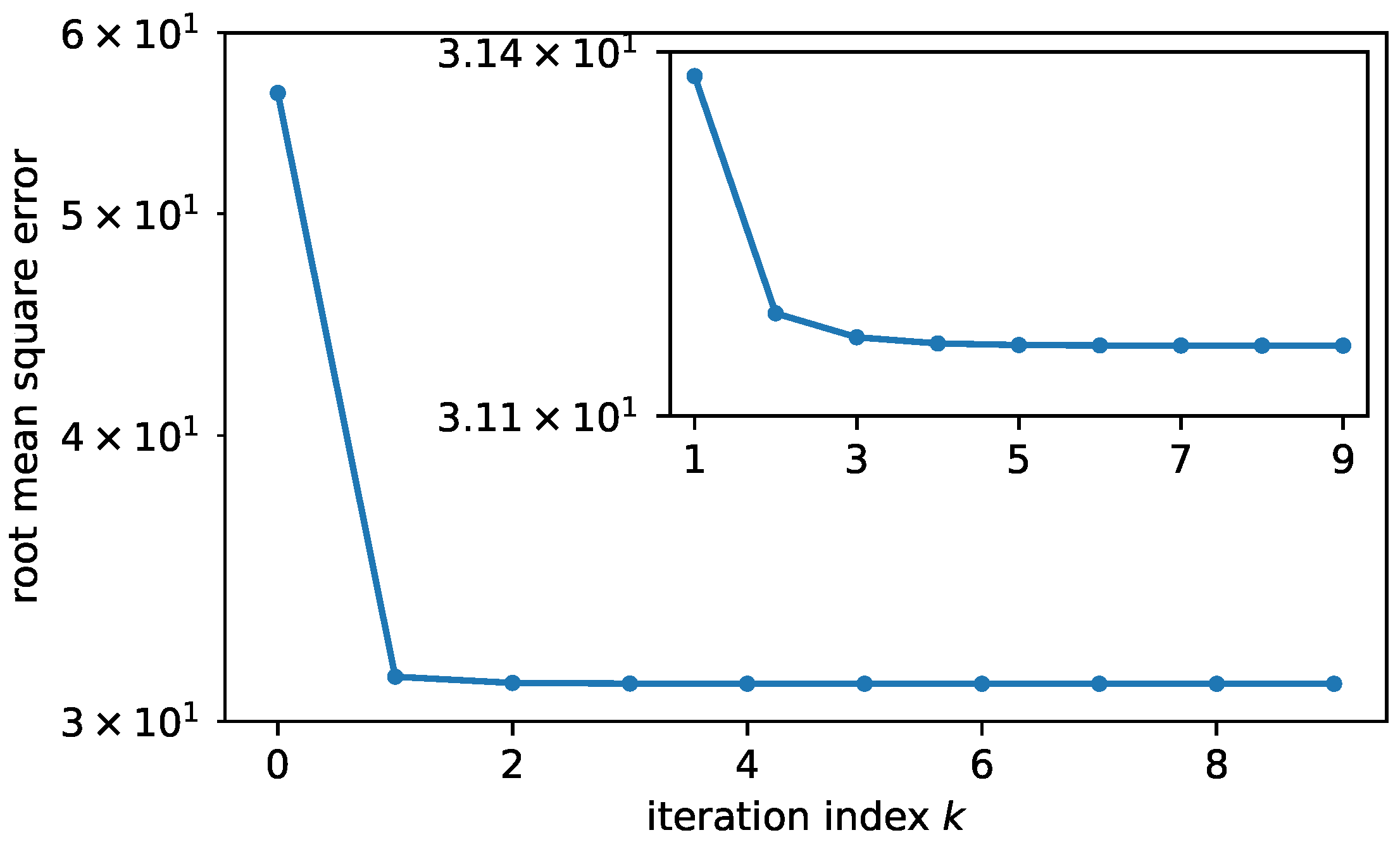
Phase stepping series of 15 images sampled at varying relative grating shifts uniformly distributed over three grating periods have been acquired both with and without sample in the beam path. Figure 1 shows the first five frames of the empty beam series. The resulting phase stepping curves at each pixel (indexed by j) of the detector have been evaluated using a least squares fit to a sinusoid model parameterized by mean , amplitude and phase offset under the initial assumption of perfectly stepped gratings. These preliminary results are shown in Figure 2 and correspond to those obtained by classic Fourier analysis of the phase stepping curves. Deviations of the sampling positions from the intended ones are then determined based on systematic deviations of the sampled data from the fitted sinusoids by means of Equation (17) for all 15 frames of the phase stepping series. Figure 6 provides an example for the first frame of the series. By iterating the sinusoid fits and the corrections to the sampling positions to reduce the overall least squares error (cf. Equation (6)) by means of Algorithm 1, the sampling positions’ deviations are found as shown in Figure 7. Figure 8 shows the reduction of Moiré modulated systematic errors in the final results, i.e., the transmission, visibility and differential phase images. The root mean square error is reduced by almost a factor of two in the present example and is already close to convergence after the first iteration as can be seen in Figure 9. Correspondingly, the deviations from the intended phase stepping positions are almost completely deduced within the first iteration, as shown in Figure 7 (bottom). Nevertheless, complete suppression of the Moiré artifacts within the final images requires some further iterations, as illustrated in Figure 10.
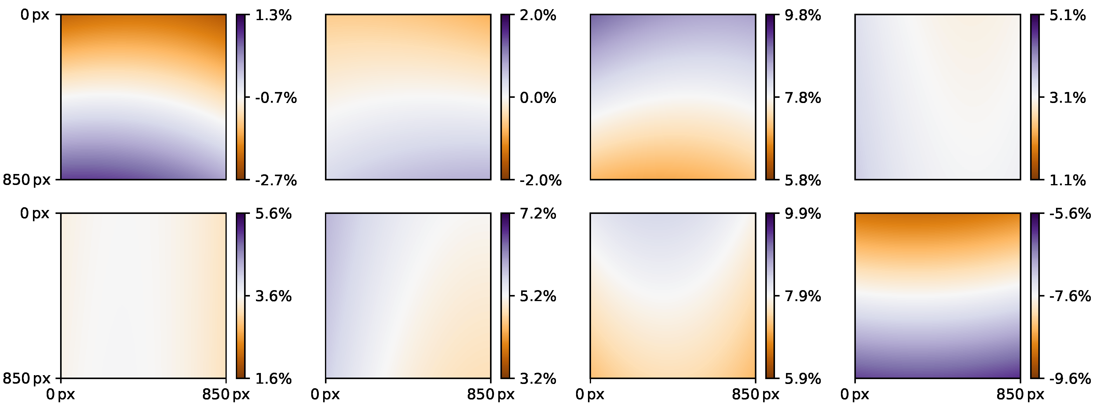
In addition to the mean deviations of the phase steps from the intended positions, spatial gradients throughout the detection area have also been considered (cf. Algorithm 2). Figure 11 shows the respective differential deviations from the intended phase steps between the first nine frames of the phase stepping series, normalized to the nominal homogeneous phase stepping increment of . The mean contributions of each component are listed in Table 1. While the homogeneous error of ranges within of the nominal step size (or of the grating period), the remaining effects are two to three orders of magnitude smaller. The root mean square error of the sinusoid fits for the whole phase stepping series is reduced by 0.1% relative to the optimization considering only homogeneous phase step deviations, as shown in Figure 9. Consequently, the derived images (not shown) are visually equivalent to those obtained previously (cf. Figure 8).
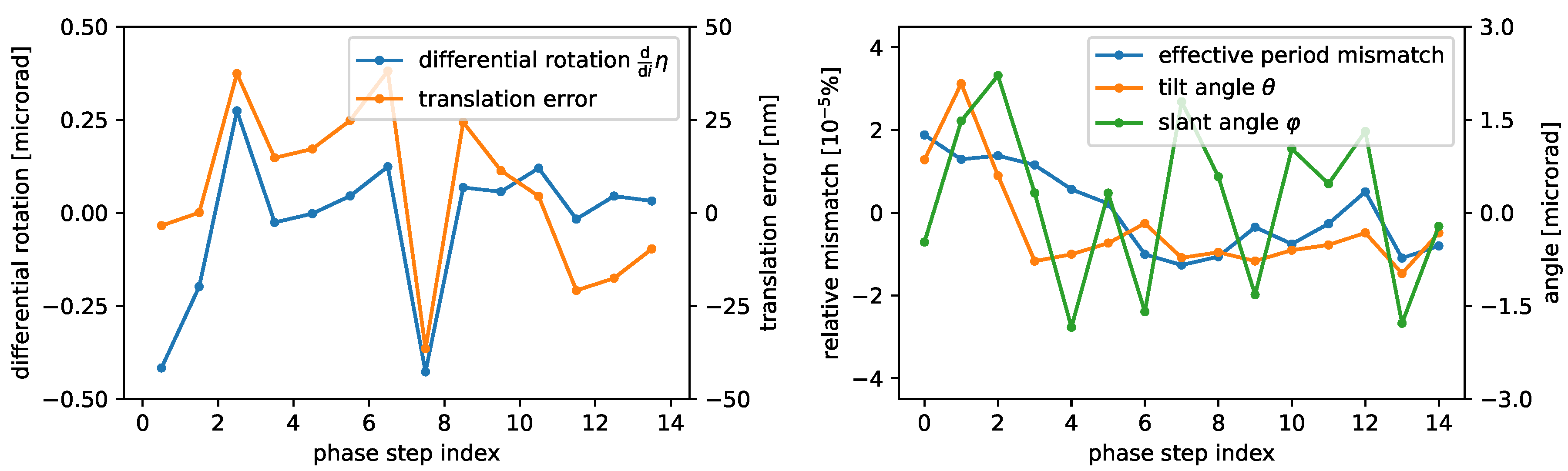
Figure 12 shows variations in the relative alignment of the gratings derived from the inhomogeneous phase stepping analysis by means of Equations (21)–(25). Besides deviations from the nominal linear motion of the gratings, minute rotations as well as subtle changes in relative magnification can also be detected. The correlation between grating rotations and translational errors visible in the left hand side graph in Figure 12 indicate rotations about an off-center pivot point about below the grating center, which is consistent with the actual placement of the phase stepping actuator in the experimental setup. Although the analog correlation between tilts about the horizontal axis and translation (along the optical axis) induced variations in magnification is much less pronounced (Figure 12, right hand side), the mean trend and magnitude are also consistent with the assumption of a pivot point below the field of view. However, the observed magnitude () of the relative mismatch of the effective grating periods is well explicable by temperature variations in the order of magnitude of given a thermal expansion coefficient in the order of magnitude of for the typical wafer materials silicon and graphite. Finally, the phase stepping inhomogeneities further suggest rotational motions about the vertical axis on the microrad scale (also shown in Figure 12).
As a crude error assessment, the standard error of the mean phase deviation can be estimated from the sinusoid fits’ root mean square error:
The latter corresponds for the present data set to about of the mean observed sinusoid amplitude, which directly translates to on the abscissa. Given the amount of detector pixels contributing to the least squares fits of within each frame of the phase stepping series, a standard error in the order of magnitude of
results. This implies that, according to the results given in Table 1, the tilt and slant contributions and are close to the expected noise level for the present case.
4. Discussion and Conclusions
A fast converging iterative algorithm for the joint optimization of both the sinusoid model parameters and the actual sampling locations for the evaluation of grating interferometric phase stepping series has been proposed. The additional effort (with respect to [5,6]) of explicitly optimizing phases rather than Fourier coefficients allows for a straight forward extension of the optimization algorithm also in the case of spatially varying phase stepping increments due to further mechanical degrees of freedom besides the intended translatory stepping motion. By division of the full optimization task into three easily tractable subproblems (phase stepping curve fitting, identification of sampling position deviations and fitting of the latter to an expected spatial model), the use of generic nonlinear optimization algorithms as, e.g., used in [7] is avoided. Of these subtasks, only the second one is actually nonlinear, and a significant portion of the present article has been devoted to its approximate linearization (also taking noise propagation into consideration). The problem of simultaneous phase stepping curve evaluation and (spatially varying) sampling position determination is thus reduced to the iterative alternation of two generalized linear least squares problems and one linear approximation to a nonlinear problem. Due to this almost linear nature, sufficient convergence is achieved within less than five iterations for the presented example. Although no rigorous convergence analysis has been performed, the outlined structure of the optimization problem does not raise severe concerns regarding its stability. In cases of doubt, convergence can simply be slowed down by means of the relaxation parameter .
For the presented example data set, mean phase stepping errors of up to 10% of the nominal step width have been found, and their correction results in both a considerable reduction of the overall root mean square error by almost a factor of two and a significant visual improvement of the final images. Although higher order effects are observable, their contribution was found to be two to three orders of magnitude smaller than that of the mean stepping error, and their correction thus did not contribute to further improvements in visual image quality in the present case. However, the higher order deviations allow the detection of minute motions of the gratings and thus provide a valuable tool for the monitoring and debugging of experimental setups. First order approximations for the relations between spatial phase variations and mechanical degrees of freedom of the moved grating have been given. For the present data set, linear motion errors up to as well as rotational motions on the microrad scale have been inferred from the phase stepping series. While the tilt and slant angles about the horizontal and vertical axes, respectively, have been found to range close to the expected noise level and should rather be interpreted as upper limits to actual motions, magnification changes in the range of and sub-microrad rotations about the optical axis were well detectable. The expected correlations between rotation and translation due to an off-center pivot point further support the plausibility of the results. This crosstalk between sub-microrad rotations and effective translations further indicates that noticeable phase stepping errors will be almost inevitable even for very carefully designed experiments, wherefore an optimization based evaluation of the phase stepping series as proposed in Algorithm 1 is generally advisable. With processing speeds in the range of per phase stepping series (using graphics processors), it is well suitable as a standard processing method also for large image series.
Author Contributions
Conceptualization, J.D., A.B. and S.Z.; Methodology, J.D.; Software, J.D.; Validation, J.D.; Formal Analysis, J.D.; Investigation, J.D. and A.B.; Resources, S.Z. and A.B.; Data Curation, J.D.; Writing—Original Draft Preparation, J.D.; Writing—Review and Editing, J.D., A.B. and S.Z.; Visualization, J.D.; Supervision, S.Z.; and Project Administration, S.Z.
Funding
The research was funded by the project group “Nano-CT Systems” (NCTS) of the Fraunhofer IIS/EZRT, which was supported by the Bavarian State ministry of Economic Affairs, Infrastructure, Transport and Technology.
Acknowledgments
The authors acknowledge R. Hanke for facilitating the present work, K. Dremel and D. Althoff for operation of the utilized in house X-ray setup and A. Haydock for proof-reading the manuscript with respect to English language. Further, the scipy libraries (http://www.scipy.org) are acknowledged, which were extensively used to perform the presented analyses.
Conflicts of Interest
The authors declare no conflict of interest.
Abbreviations
The following abbreviations are used in this manuscript:
| PSC | Phase stepping curve |
| RMSE | Root mean square error |
References
- David, C.; Nöhammer, B.; Solak, H.H.; Ziegler, E. Differential x-ray phase contrast imaging using a shearing interferometer. Appl. Phys. Lett. 2002, 81, 3287–3289. [Google Scholar] [CrossRef]
- Momose, A.; Kawamoto, S.; Koyama, I.; Hamaishi, Y.; Takai, K.; Suzuki, Y. Demonstration of X-Ray Talbot Interferometry. Jpn. J. Appl. Phys. 2003, 42, L866–L868. [Google Scholar] [CrossRef]
- Pfeiffer, F.; Weitkamp, T.; Bunk, O.; David, C. Phase retrieval and differential phase-contrast imaging with low-brilliance X-ray sources. Nat. Phys. 2006, 2, 258–261. [Google Scholar] [CrossRef] [Green Version]
- Revol, V.; Kottler, C.; Kaufmann, R.; Straumann, U.; Urban, C. Noise analysis of grating-based x-ray differential phase contrast imaging. Rev. Sci. Instrum. 2010, 81, 073709. [Google Scholar] [CrossRef] [PubMed]
- Seifert, M.; Kaeppler, S.; Hauke, C.; Horn, F.; Pelzer, G.; Rieger, J.; Michel, T.; Riess, C.; Anton, G. Optimisation of image reconstruction for phase-contrast x-ray Talbot–Lau imaging with regard to mechanical robustness. Phys. Med. Biol. 2016, 61, 6441–6464. [Google Scholar] [CrossRef] [PubMed]
- Vargas, J.; Sorzano, C.O.S.; Estrada, J.C.; Carazo, J.M. Generalization of the Principal Component Analysis algorithm for interferometry. Opt. Commun. 2013, 286, 130–134. [Google Scholar] [CrossRef]
- Kaeppler, S.; Rieger, J.; Pelzer, G.; Horn, F.; Michel, T.; Maier, A.; Anton, G.; Riess, C. Improved reconstruction of phase-stepping data for Talbot-Lau x-ray imaging. J. Med. Imaging 2017, 4, 034005. [Google Scholar] [CrossRef] [PubMed]
- Von Teuffenbach, M.; Noichl, W.; Brendel, B.; Herzen, J.; Pfeiffer, F.; Koehler, T.; Noël, P.B. Grating Position Estimation for Grating-based Computed Tomography. In Proceedings of the Conference on X-ray and Neutron Phase Imaging with Gratings, XNPIG 2017, Zurich, Switzerland, 12–15 September 2017; pp. 169–170. [Google Scholar]
- Ritter, A.; Anton, G.; Weber, T. Simultaneous Maximum-Likelihood Reconstruction of Absorption Coefficient, Reconstruction of Absorption Coefficient, Refractive Index and Dark-Field Scattering Coefficient in X-Ray Talbot-Lau Tomography. PLoS ONE 2016, 11, e0163016. [Google Scholar] [CrossRef] [PubMed]
- Marco, F.D.; Marschner, M.; Birnbacher, L.; Noël, P.; Herzen, J.; Pfeiffer, F. Analysis and correction of bias induced by phase stepping jitter in grating-based X-ray phase-contrast imaging. Opt. Express 2018, 26, 12707–12722. [Google Scholar] [CrossRef] [PubMed]
- Yashiro, W.; Terui, Y.; Kawabata, K.; Momose, A. On the origin of visibility contrast in x-ray Talbot interferometry. Opt. Express 2010, 18, 16890–16901. [Google Scholar] [CrossRef] [PubMed]
- Bech, M.; Bunk, O.; Donath, T.; Feidenhans’l, R.; David, C.; Pfeiffer, F. Quantitative x-ray dark-field computed tomography. Phys. Med. Biol. 2010, 55, 5529–5539. [Google Scholar] [CrossRef] [PubMed]
- Strobl, M. General solution for quantitative dark-field contrast imaging with grating interferometers. Sci. Rep. 2014, 4, 7243. [Google Scholar] [CrossRef] [PubMed] [Green Version]
- Jensen, T.H.; Bech, M.; Bunk, O.; Donath, T.; David, C.; Feidenhans’l, R.; Pfeiffer, F. Directional x-ray dark-field imaging. Phys. Med. Biol. 2010, 55, 3317–3323. [Google Scholar] [CrossRef] [PubMed]
- Revol, V.; Kottler, C.; Kaufmann, R.; Neels, A.; Dommann, A. Orientation-selective X-ray dark field imaging of ordered systems. J. Appl. Phys. 2012, 112, 114903. [Google Scholar] [CrossRef]
- Malecki, A.; Potdevin, G.; Biernath, T.; Eggl, E.; Willer, K.; Lasser, T.; Maisenbacher, J.; Gibmeier, J.; Wanner, A.; Pfeiffer, F. X-ray tensor tomography. Europhys. Lett. 2014, 105, 38002. [Google Scholar] [CrossRef]
- Bayer, F.; Hu, S.; Maier, A.; Weber, T.; Anton, G.; Michel, T.; Riess, C. Reconstruction of scalar and vectorial components in X-ray dark-field tomography. Proc. Natl. Acad. Sci. USA 2014, 111, 12699–12704. [Google Scholar] [CrossRef] [PubMed] [Green Version]
- Vogel, J.; Schaff, F.; Fehringer, A.; Jud, C.; Wieczorek, M.; Pfeiffer, F.; Lasser, T. Constrained X-ray tensor tomography reconstruction. Opt. Express 2015, 23, 15134–15151. [Google Scholar] [CrossRef] [PubMed]
- Wieczorek, M.; Schaff, F.; Pfeiffer, F.; Lasser, T. Anisotropic X-ray Dark-Field Tomography: A Continuous Model and its Discretization. Phys. Rev. Lett. 2016, 117, 158101. [Google Scholar] [CrossRef] [PubMed]
- Sharma, Y.; Wieczorek, M.; Schaff, F.; Seyyedi, S.; Prade, F.; Pfeiffer, F. Six dimensional X-ray Tensor Tomography with a compact laboratory setup. Appl. Phys. Lett. 2016, 109, 134102. [Google Scholar] [CrossRef] [Green Version]
- Dittmann, J.; Zabler, S.; Hanke, R. Nested Tomography: Application to Direct Ellipsoid Reconstruction in Anisotropic Darkfield Tomography. In Proceedings of the Conference on X-ray and Neutron Phase Imaging with Gratings, XNPIG 2017, Zurich, Switzerland, 12–15 September 2017; pp. 49–50. [Google Scholar]
Figure 1.
Example for a grating interferometric phase stepping series (without sample, cf. Section 2.3 for experimental details). The intensity variation throughout the series is visually most perceivable in the center. The Moiré fringes are caused by imperfectly matched gratings and will translate to reference offset phases of the sinusoid curves found at each detector pixel (cf. Figure 2). The bottom panel shows a corresponding phase stepping curve for the pixel marked orange in the above image series. The sampling positions are subject to an unknown error.
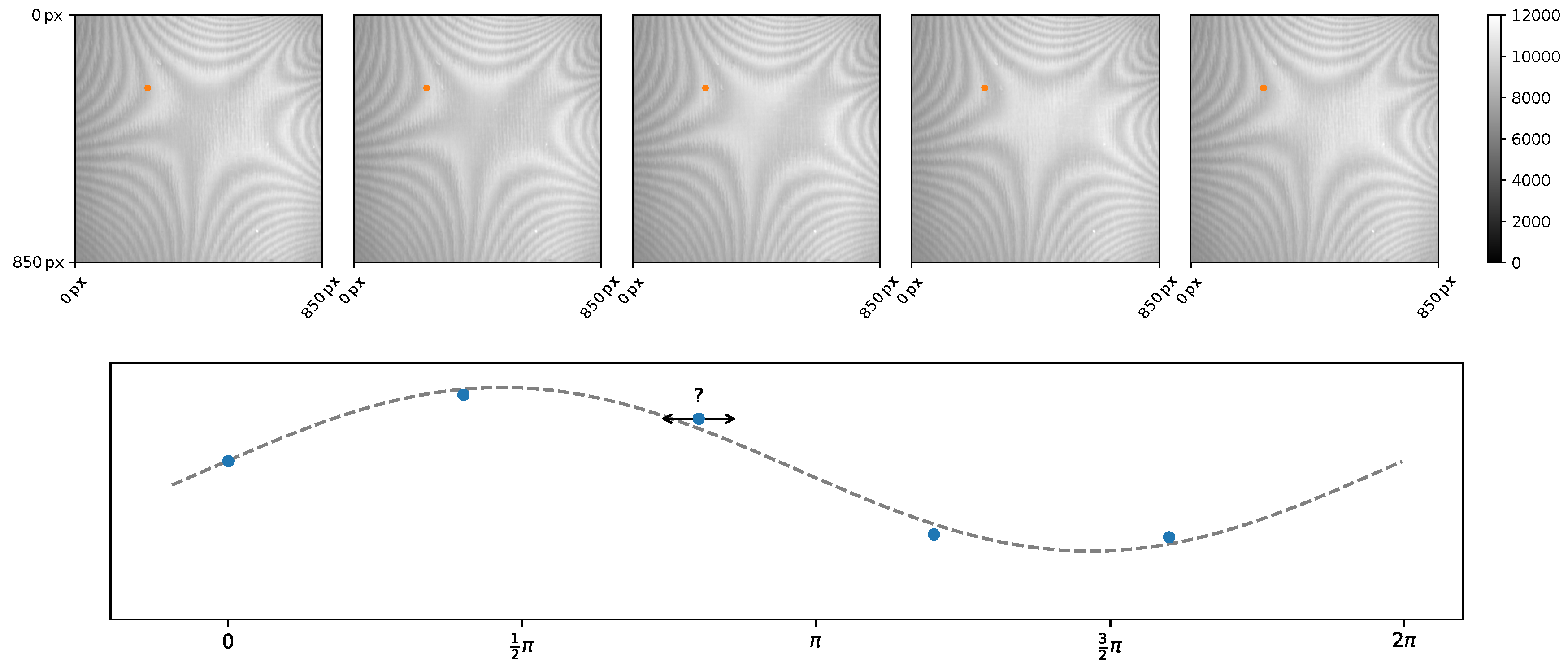
Figure 2.
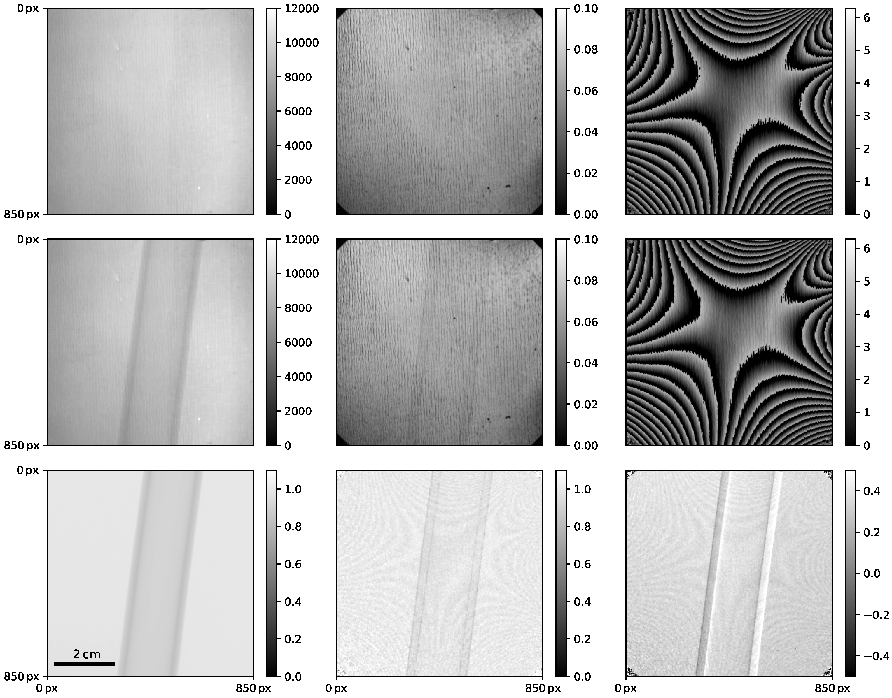
From left to right: Transmission (sinusoid mean), visibility (ratio of sinusoid amplitude and mean) and phase images derived from phase stepping series, as shown in Figure 1. The first two rows show acquisitions with and without sample (a piece of plastic hose of 2 cm diameter), while the last row shows the sample images (center row) normalized with respect to the empty beam images (first row). Positioning errors in the phase stepping procedure cause the Moiré pattern of the reference phase image to translate into the final results.
Figure 2.
From left to right: Transmission (sinusoid mean), visibility (ratio of sinusoid amplitude and mean) and phase images derived from phase stepping series, as shown in Figure 1. The first two rows show acquisitions with and without sample (a piece of plastic hose of 2 cm diameter), while the last row shows the sample images (center row) normalized with respect to the empty beam images (first row). Positioning errors in the phase stepping procedure cause the Moiré pattern of the reference phase image to translate into the final results.

Figure 3.
Optimization of the actual (in contrast to the intended) sampling positions by Equation (14) with respect to a previous sinusoid fit based on the temporary assumption that deviations from the sinusoid model are mainly due to errors on the sampling positions rather than the sampled ordinate values. Averaging of respective phase deviations found for large sets of measurements will finally allow the differentiation of systematic deviations from statistical noise.

Figure 4.
Illustration of the maximal sensible ranges for linear approximations of a sinusoid. Vertical lines at the turning points indicate the boundaries of monotone sections that should never be crossed by linear approximations of the curve. The maximum meaningful range is thus largest for points furthest from these boundaries and reduces to zero exactly at the turning points. Equation (12) approximates this phase dependence of the validity range with a function, and Equation (13) defines the maximum amplitude admissible to indeed never exceed turning points.
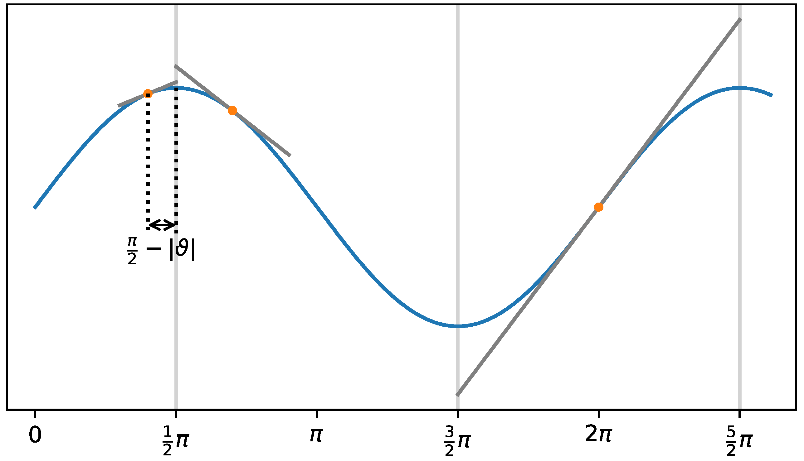
Figure 5.
Grating misalignments (top row) and corresponding spatial phase variations (bottom row). From left to right: Translation, magnification, rotation, tilt, and slant. The latter two effects (as well as translation induced magnification) are only observable in cone beam setups. The employed color bar ranges from orange for negative values over white (zero) to blue for positive values.

Figure 6.
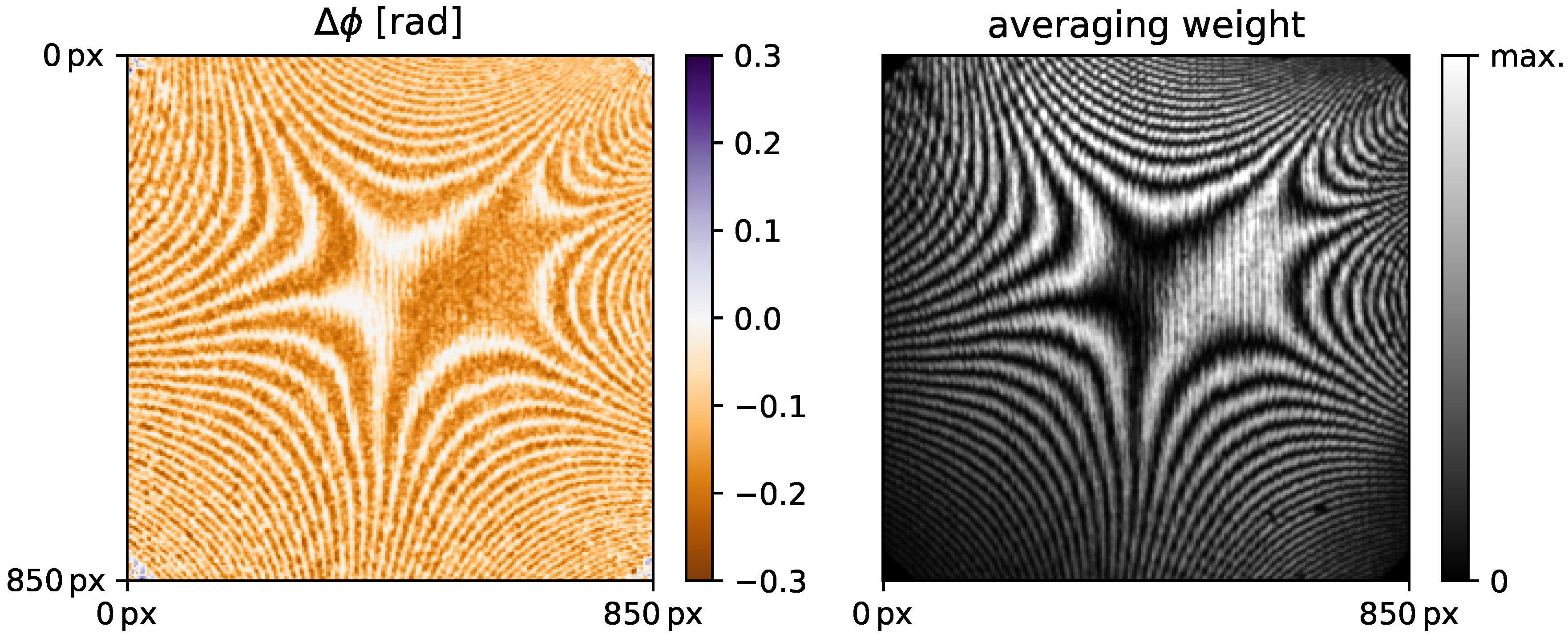
Example of sampling phase deviations (left) obtained from Equation 14 (cf. also Figure 3) for the first frame of the phase stepping series shown in Figure 1 with corresponding importance weights (right) as defined by Equation (16). White regions (0 on the colorbar) in the map (left) correspond to samples close to or exactly on turning points of the fitted sinusoids, where phase deviations cannot be effectively determined. These areas get little weighting in the determination of the average phase deviation as can be seen by the corresponding dark fringes in the weighting map on the right.
Figure 6.
Example of sampling phase deviations (left) obtained from Equation 14 (cf. also Figure 3) for the first frame of the phase stepping series shown in Figure 1 with corresponding importance weights (right) as defined by Equation (16). White regions (0 on the colorbar) in the map (left) correspond to samples close to or exactly on turning points of the fitted sinusoids, where phase deviations cannot be effectively determined. These areas get little weighting in the determination of the average phase deviation as can be seen by the corresponding dark fringes in the weighting map on the right.

Figure 7.
Above: An example phase stepping curve consisting of 15 steps over three grating periods. Sampled values are shown both at the originally intended as well as at the inferred sampling positions (blue and orange markers respectively) along with the corresponding initial and corrected sinusoid fits. Although the difference in the resulting fit appears small, it is clearly noticeable in the final images, as shown in Figure 8. Below: Deviations of the phase stepping series’ sampling positions from the intended ones in units of radians as found at 0, 1 and 9 iterations of Algorithm 1. The range of deviations corresponds to roughly of the intended stepping increments of .
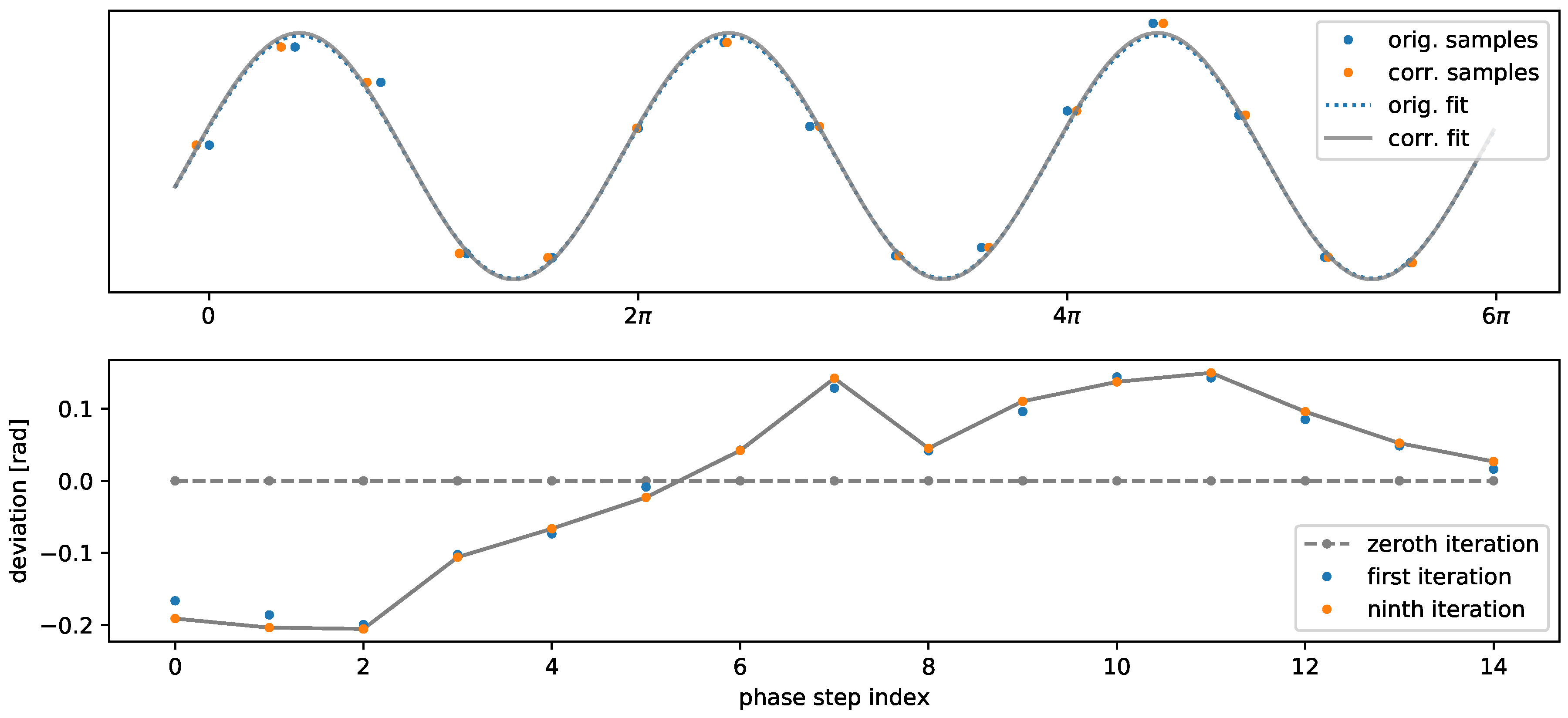
Figure 8.
Transmission, visibility and phase images (from left to right) of the sample referenced to empty beam images. The top and bottom rows show results based on phase stepping curve evaluations with and without correction of the actual sampling positions, respectively. The evaluation based on the assumption of error free sampling positions (bottom row) exhibits distinctive systematic errors modulated by the Moiré structure of the reference phase image (cf. Figure 2).
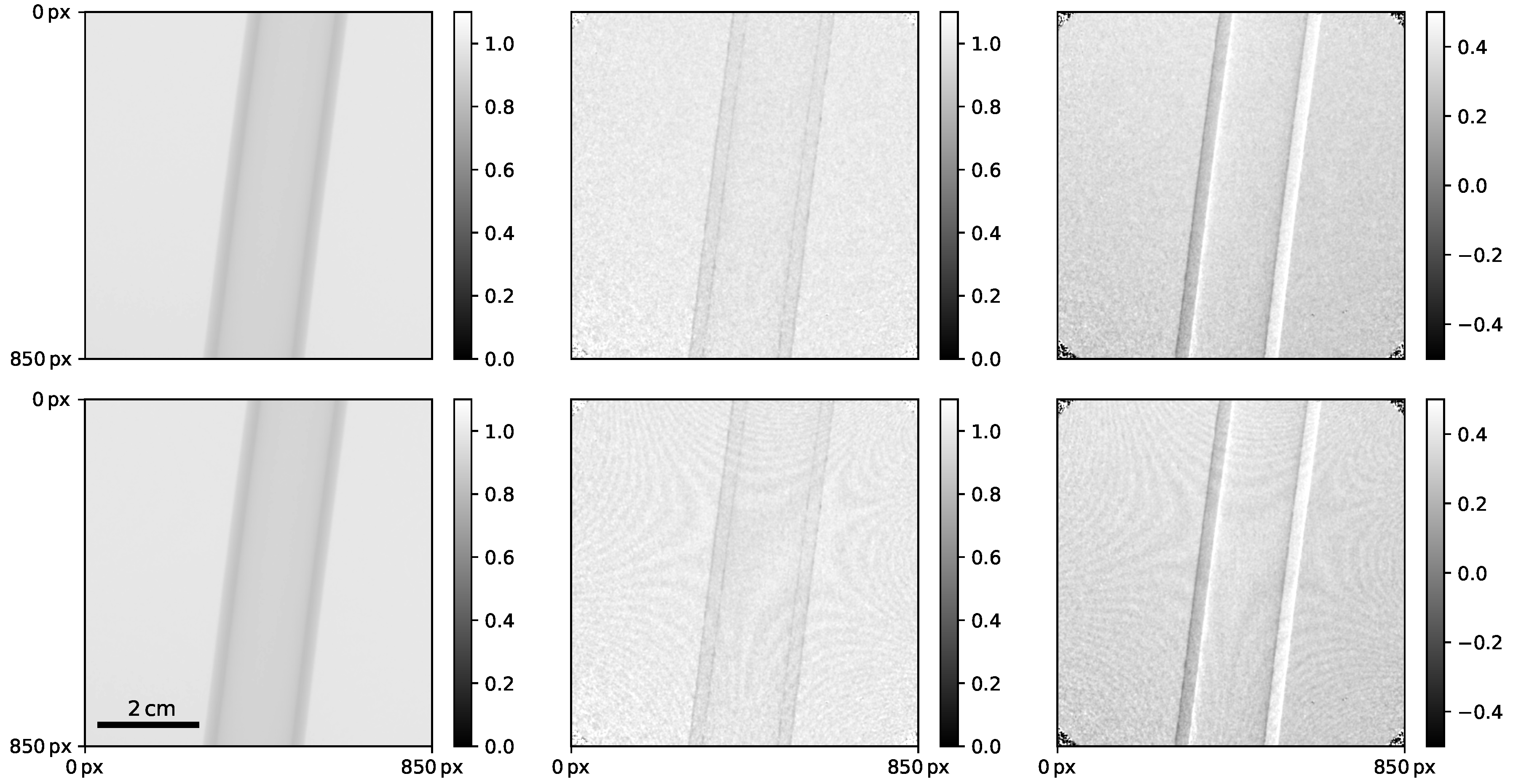
Figure 9.
Root mean square error (RMSE) of the sinusoid fits to the empty beam phase stepping series throughout the iterations of Algorithm 1. After the first correction of the actual sampling locations by Equation (17), the error is reduced by almost a factor of two. The following iterations further reduce the error confirming the validity of Algorithm 1 for the solution of Equation (6). Additional consideration of spatially inhomogeneous stepping distances (Equation (2)) further reduces the RMSE by merely 0.1%.

Figure 10.
From left to right: Visibility images normalized to the respective empty beam images for 0 (regular analysis assuming perfect stepping), 1, 3 and 9 iterations of Algorithm 1 applied to the phase stepping series with and without sample, respectively. The grayscale window has been chosen to emphasize the Moiré artifacts.
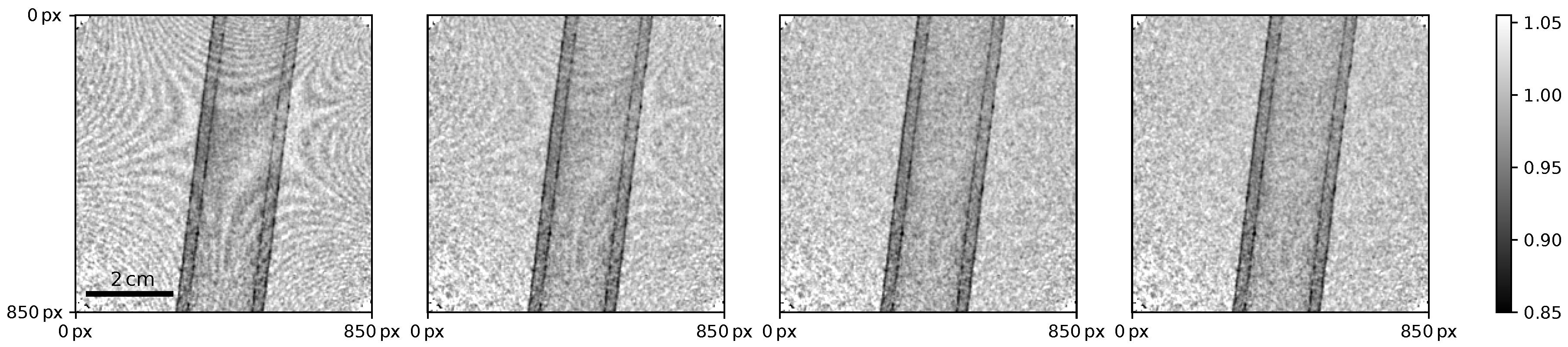
Figure 11.
Relative deviations of the actual phase steps from the intended step width of between the first nine frames of the phase stepping series (). The variations have been determined by optimization of Equation (18) assuming the spatial dependence defined by Equation (19) (see also Algorithm 2).

Figure 12.
Quantitative results derivable from the inhomogeneities in the phase stepping deviations (Equation (19)). On the left, the change in tilt angle about the optical axis from frame to frame within the phase stepping series is shown along with the accompanying linear motion error. Rotation correlated translations indicate an off-center pivot point. On the right hand side, the relative grating scaling error is shown along with the found tilt and slant about the horizontal and vertical axis. These quantities represent deviations from the mean grating alignment throughout the phase stepping series. The tilt and slant angles range close to the expected noise level (cf. Table 1 and Equation (27)).


Table 1.
Root mean square contributions of the mean, gradient and curvature components of to the sampling phase deviations found for the present phase stepping series in units of radians. The homogeneous error is by far the dominating effect. The contributions of and range in the order of magnitude of the expected noise level of (cf. Equations (26) and (27)).
© 2018 by the authors. Licensee MDPI, Basel, Switzerland. This article is an open access article distributed under the terms and conditions of the Creative Commons Attribution (CC BY) license (http://creativecommons.org/licenses/by/4.0/).
Share and Cite
MDPI and ACS Style
Dittmann, J.; Balles, A.; Zabler, S. Optimization Based Evaluation of Grating Interferometric Phase Stepping Series and Analysis of Mechanical Setup Instabilities. J. Imaging 2018, 4, 77. https://doi.org/10.3390/jimaging4060077
AMA Style
Dittmann J, Balles A, Zabler S. Optimization Based Evaluation of Grating Interferometric Phase Stepping Series and Analysis of Mechanical Setup Instabilities. Journal of Imaging. 2018; 4(6):77. https://doi.org/10.3390/jimaging4060077
Chicago/Turabian StyleDittmann, Jonas, Andreas Balles, and Simon Zabler. 2018. "Optimization Based Evaluation of Grating Interferometric Phase Stepping Series and Analysis of Mechanical Setup Instabilities" Journal of Imaging 4, no. 6: 77. https://doi.org/10.3390/jimaging4060077
Note that from the first issue of 2016, this journal uses article numbers instead of page numbers. See further details here.