Feature Importance for Human Epithelial (HEp-2) Cell Image Classification ^†

Abstract

Indirect Immuno-Fluorescence (IIF) microscopy imaging of human epithelial (HEp-2) cells is a popular method for diagnosing autoimmune diseases. Considering large data volumes, computer-aided diagnosis (CAD) systems, based on image-based classification, can help in terms of time, effort, and reliability of diagnosis. Such approaches are based on extracting some representative features from the images. This work explores the selection of the most distinctive features for HEp-2 cell images using various feature selection (FS) methods. Considering that there is no single universally optimal feature selection technique, we also propose hybridization of one class of FS methods (filter methods). Furthermore, the notion of variable importance for ranking features, provided by another type of approaches (embedded methods such as Random forest, Random uniform forest) is exploited to select a good subset of features from a large set, such that addition of new features does not increase classification accuracy. In this work, we have also, with great consideration, designed class-specific features to capture morphological visual traits of the cell patterns. We perform various experiments and discussions to demonstrate the effectiveness of FS methods along with proposed and a standard feature set. We achieve state-of-the-art performance even with small number of features, obtained after the feature selection.

1. Introduction

Antinuclear antibody (ANA) detection with an HEp-2 substrate, is used as a standard test to reveal the presence of auto-immune antibodies. If antibodies are present in the blood serum of the patient, their presence manifests in distinct nuclear staining patterns of fluorescence on the HEp-2 cells [1]. Owing to higher sensitivity of HEp-2 cell lines, ANA determination by indirect immunofuorescence (IIF) is arguably the most popular initial screening test for suspected autoimmune diseases (such as Myasthenia gravis, Pernicious anemia, Reactive arthritis, Sjogren syndrome) [2]. The key step of the ANA HEp-2 medical test is the interpretation of obtained stained patterns of HEp-2 cells for establishing a correct diagnosis. The ANA HEp-2 test produces diverse staining patterns due to staining of different cell regions or domains. These domains such as nucleoli, nucleus, cytosol and chromosomes, differ in size, shape, number and localization inside the cell. This allows interpreters to distinguish staining patterns characteristic for different autoimmune deceases. Classifying these patterns using computer-aided diagnosis (CAD) systems has important clinical applications as manual evaluation demands long hours causing fatigue, and is also highly subjective. Being a second opinion system, the CAD systems reduce the workload of specialists, contributing to both diagnosis efficiency and cost reduction.

As such, many different staining patterns (approximately 30–35) are reported [3,4], on the basis of the formation of molecular complex at different sites. However, it is observed that only few of these staining patterns are clinically more significant and are often detected by indirect immunofuorescence (IIF) microscopy on HEp-2 cells in the sera of patients with autoimmune disease [5]. Perhaps, this is the reason why a standard publicly available dataset [6] also provide images only with respect to these six patterns viz. Homogeneous, Speckled, Nucleolar, Centromere, Nuclear Membrane and Golgi. In our work, we use this dataset. Figure 1 depicts examples of these fluorescence staining patterns, where the task is to classify a given test cell image into one of these six classes.

The characteristic definitions of some fluorescence patterns based on its visual traits, can be stated as follows [3,7]:

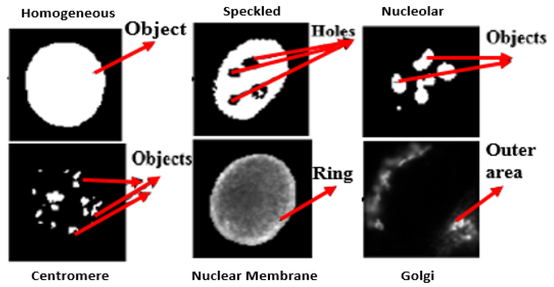
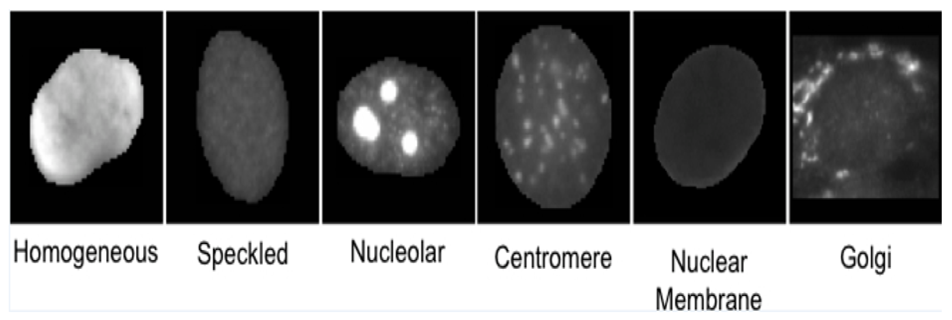
• Homogeneous: A uniformly diffused fluorescence covering the entire nucleoplasm sometimes accentuated in the nuclear periphery.
• Speckled: This pattern can be explained under two categories (which, however, are not separately labeled in the dataset)

  -

  Coarse speckled: Density distributed, various sized speckles, generally associated with larger speckles, throughout nucleoplasm of inter-phase cells; nucleoli are negative.

  -

  Fine speckled: Fine speckled staining in a uniform distributed, sometimes very dense so that an almost homogeneous pattern is attained; nucleoli may be positive and negative.

• Nucleolar: Characterized by clustered large granules in the nucleoli of inter phase cells which tend towards homogeneity, with less than six granules per cell.
• Centromere: Characterized by several discrete speckles (40–60) distributed throughout the inter phase nuclei.
• Nuclear Membrane: A smooth homogeneous ring-like fluorescence at the nuclear membrane.
• Golgi: Staining of polar organelle adjacent to and partly surrounding the nucleus, composed of irregular large granules. Nuclei and nucleoli are negative.

In addition to the classification of the above depicted interphase staining patterns, the diagnostic procedure based on ANA IIF images also involves an initial step of mitotic cells recognition. The mitotic cell recognition step is important for two reasons. First, the presence of at least one mitotic cell indicates a well prepared sample [8]. While the mitotic detection (a binary classification problem) is important as is shown in some recent works [9,10], in this work, we focus on the multi-class interphase cell classification problems, which is also, in itself, important from the perspective of Auto-immune disease diagnosis. Indeed the importance of the interphase classification problem is indicated by the presence of relatively large dataset that we use in this work [6], which only contains cell images of interphase patterns.

Feature extraction plays an important role in the classification of staining patterns. It is a process that transforms the raw input data into a set of features. The generated feature set encodes numerous important and relevant characteristics and distinctive properties of raw data that help in differentiating between the categories of input patterns. To represent such characteristics for HEp-2 cell images, various automated methods have been developed which typically compute large number of standard image-based features (e.g., morphology, texture and other sophisticated features like (Scale-invariant feature transform (SIFT) [11], Stein’s unbiased risk estimate (SURE) [11], Local Binary Pattern (LBP) [12], Histogram of oriented gradients (HOG) etc.).

We note that variations existing within the input patterns of cell images are typically reflected in terms of visual traits for morphology or texture. We can notice many features within the staining patterns which have various distinct morphological traits such as differences in area of foreground (white) pixels, size of granules (object), number of granules (object) etc. In this work, we have employed some class-specific features, formulated in one of our previous work [13], and some texture features [14] to represent such visual traits in order to discriminate the classes of HEp-2 cells.

1.1. Feature Selection

Out of a large amount of feature extraction, it often turns out that all features may not always be relevant for discrimination. If carefully chosen, a reduced feature set can perform the desired task. Thus, the task of feature selection (FS) aims to find a feature subset that can describe the data for a learning task more compactly than the original set. As indicated above, in the present task, as there can be numerous features to characterize cell morphology and texture, we have primarily focused on the feature selection among these.

Feature selection can induce following benefits [15,16]: (1) Improved classification performance due to removal of unreliable features that can negatively affect the performance; (2) Reduced dimensionality of the feature space, leading to reducing the test-phase computation and storage; (3) Removal of redundant features often leads to better generalization ability towards new samples; (4) Better interpretibility of the classification problem, considering a smaller number of features.

Feature selection algorithms can be categorized into two groups, i.e., supervised and unsupervised feature selection [15]. Supervised feature selection algorithms are based on using discriminative information enclosed in labels. Below, we discuss some of these in brief:

• Filtering methods that use statistical properties of features to assign a score to each feature. Some examples are: information gain, chi-square test [17], fisher score, correlation coefficient, variance threshold etc. These methods are computationally efficient but do not consider the relationship between feature variables and response variable.
• Wrapper methods explore whole feature space to find an optimal subset by selecting features based on the classifier performance. These methods are computationally expensive due to the need to train and cross-validate model for each feature subset. Some examples are: recursive feature elimination, sequential feature selection [18] algorithms, genetic algorithms etc.
• Embedded methods perform feature selection as part of the learning procedure, and are generally specific for given classifier framework. Such approaches are more elegant than filtering methods, and computationally less intensive and less prone to over-fitting than wrapper methods. Some examples are: Random Forests [19] for Feature Ranking, Recursive Feature Elimination (RFE) with SVM, Adaboost for Feature Selection etc.

In unsupervised scenario, however, no label information is used, and feature selection involves approaches such as clustering, spectral regression, exploitation of feature correlations etc. Various feature selection methods in unsupervised domain have been reported in the literature. Some of these methods, which we consider are: Infinite Feature Selection (InFS) [20], Regularized Discriminative Feature Selection (UDFS) [21], Multi Class/Cluster feature selection (MCFS) [22]. Note that a reduced representation may also be obtained by some dimensionality reduction techniques that are based on projection of features into a subspace (e.g., principal component analysis) or compression (e.g., using information theory). However, unlike these, the feature selection techniques do not alter the original representation of the variables, but merely select a subset of them. Hence, they preserve the original semantics of the features, and do not lose on the advantage of interpretability.

1.2. Scope of the Work

The primary focus of this paper is to consider the effectiveness of different feature selection (FS) methods from perspective of HEp-2 cell image classification. This work involves various traditional and contemporary methods of feature selection among the categories mentioned above, including chi square test, t-test, information gain, sequential forward search (SFS), random subspace feature selection (RSFS) and variants on Random Forests. This study focuses to explore the features selection aspect considering the possibility of improvement in the classification process over the case which employs a complete set of baseline features. In this study, we consider both supervised and unsupervised feature selection methods.

Knowing that, there is often not a single universally optimal feature selection technique [23], it is useful to consider the hybridization of some FS methods, which can yield a more compact feature subset. This aspect is inspired by ensemble learning where, in a similar spirit, various classifiers are integrated to obtain a stronger classifier.

Motivated by this aspect, we propose a hybridization approach for a class of FS method, viz. the filter based FS methods. We consider only filter methods for the hybridization, as these methods are potentially adhoc, i.e., they provide feature ranking, but the selection of an optimal set of features is decided by an empirical threshold on feature ranking (score). The hybridization combines various filter methods to get a more robust feature ranking. The problem of adhoc threshold selection is also addressed by the hybridization approach as it automatically selects an eventual feature subset.

In addition, as discussed above, embedded algorithms provide feature importance by the internal mechanisms of the classification algorithm. For example, decision trees and their variants such as random forests [19], random uniform forest [24] perform recursive segregation of the given information by focusing on the features which have more potential to discriminate between the two classes. These methods are less intensive and much less prone to over-fitting. In this work, we have demonstrated an ability of Random Forest (RF) and Random Uniform Forest (RUF) for selecting an important discriminative feature set and thereby examine the contribution of each feature for the application of HEp-2 cell image classification. Unlike the existing works on HEp-2 cell classification, we stress on the feature selection aspect of random forest. Moreover, we also propose to utilize another variant of the random forest (viz. random uniform forest) for this work, which yields a superior performance over the standard random forest.

The choice of RF for this study is due to its various advantages over other classifiers such as, (1) From the feature selection perspective, RF inherently involves the notion of variable importance together with classification accuracy, which tells about how much the accuracy will degrade when a particular feature is removed from the feature set. By choosing the features which have higher ranks, an optimal subset can be found. (2) It has less parameters to tune (number and depth of trees), as compared to ensemble structures with popular classifiers (e.g., SVM, neural networks) where number of classifiers, choice of kernel and its parameters, cost function, number of hidden layers, number of nodes in the hidden layers etc. require tuning. In this work, we only tune the number of trees. (3) For a large dataset, it can be parallelized, and it can easily handle uneven data sets that have missing variables and mixed data (although this is not relevant in the current work). (4) It is known to perform well across various domains.

In addition to our study on feature selection, we focus on using simple feature definitions and training data (40%), and demonstrate state-of-the-art performance with the same. We believe that such a direction of feature selection is interesting, given that this is a emerging research area.

Summary of contribution: (1) Exploring various feature selection (FS) techniques for the task of HEp2 cell image classification, (2) Hybridization technique to combine filter based FS techniques to automatic select feature subset, (3) Utilization of random forest and random uniform forests for feature selection for HEp-2 cell image classification, (4) Employing simplistic and visually more interpretable feature definitions, yielding state-of-the-art performance. (5) Experimental analysis including, (a) Demonstration of performance using low dimensional and high dimensional feature sets, (b) Providing an insightful discussion on the performance of various FS methods (c) Positive comparison with state-of-the-art methods.

This paper is a significantly extended version of our earlier work [25] published in the proceedings of the Int. Conf. on Medical Image Understanding and Analysis (MIUA) 2017. In [25], we have reported only random forest based feature selection for classification of HEp-2 cell images. The present work explores various feature selection methods for this classification task, and provides insightful discussions and comparisons.

2. Related Work

This section discusses some previous work, including state-of-the-art methods, aiming to automate the IIF diagnostic procedure in the context of ANA testing. Perner et al. [26] presented an early attempt in this direction. They introduced various sets of features which were extracted from cell region using multilevel gray thresholding and then used a data mining algorithm to find out the relevant features among large feature sets. Huang et al. [27] utilized 14 textural and statistical features along with self-organizing map to classify the fluorescence patterns whereas, in [28] learning vector quantization (LVQ) with eight textural features was used to identify the fluorescence pattern. The methods discussed above are evaluated on private dataset which makes performance comparison very difficult. Recently, the contests on HEp-2 cell classification [3,29], held in conjunction with the ICPR-2012, ICIP-2013, and ICPR-2014, released public datasets which are suitable for evaluation of methods as a part of relevant contests. These contests have given a strong impetus in the development of algorithms for the HEp-2 cell image classification task. Since the ICPR-2014 dataset (same as the ICIP-2013 dataset) is the most recent and of much larger scale than that of ICPR12, we use this dataset for validation and compare our framework. This is similar to other works such as [11,30,31,32,33,34] which also use the same dataset. More recent reviews of this topic were provided by [6,35].

In this context, several new approaches were proposed for cell classification and evaluated on common basis.

The reader can refer to [36] for an overview of the literature and of the open challenges in this research area. Below, we discuss some specific works in terms of features and classifiers.

While the area of HEp-2 cell image classification has been somewhat explored, to the best of our knowledge, such a study on feature selection, yielding a good classification performance has not been reported. Random forest has only been utilized as classifier for this problem. Prasath et al. [30] utilized texture features such as rotational invariant co-occurrence (RIC) versions of the well-known local binary pattern (LBP), median binary pattern (MBP), joint adaptive median binary pattern (JAMBP), and motif co-occurrence matrix (MCM) along with other optimized features, and reported mean class accuracy using different classifiers such as the k-nearest neighbors (kNN), support vector machine (SVM), and random forest (RF). The highest accuracy is obtained with RIC-LBP combined with a RIC variant of MCM. In [14] authors utilized large pool of feature and used random forest as classifier. They have achieved a good accuracy, but the work uses the ICPR-2012 dataset, which is much smaller than the one which we use (ICPR-2013/ICPR-2014) for validation, and employs a leave-one-out cross validation, thus involving a large amount of training data. Bran et al. [31] made use of the wavelet scattering network, which gives rotation-invariant wavelet coefficients as representations of cell images. The work in [32] extracted various features (Shape and Size, Texture, Statistical, LBP, HOG, and Boundary) and used the random forest for classification. Note that above discussed methods employ Random Forests, as done in a part of this work. However, it is used only as a classifier and the feature selection aspect is not considered.

In [11,33,34] authors achieved state-of-art performance for HEp-2 cell image classification In [11], Bag of Words model based on sparse coding was proposed. They used scale-invariant feature transform (SIFT) and speeded-up robust features (SURF) features with sparse coding and max pooling. Siyamalan et al. [33] presented an ensembles of SVMs based on sparse encoding of texture features with cell pyramids, capturing spatial, multi-scale structure for HEp-2 cell classification and reported mean accuracy. Diego et al. [37] utilized a biologically-inspired dense local descriptor for characterization of cell images. In  [34], authors utilized deep convolution neural network for cell classification. All the above discussed methods were bench-marked with the ICIP-2013/ICPR-2014 dataset.

The feature selection ability of RF has been reported in some other domains such as gene selection [38], breast cancer diagnosis [39,40], and analyzing radar data [41], which inspires us to explore it for the problem of HEp-2 cell image classification. In [42,43], authors provided survey on importance of feature selection, review of feature selection methods and their utilization in various fields.

Most of the feature selection methods considered here have been applied to different domains. However, the direction of feature selection has not been explored for the cell classification problem. We believe that reduction in number of features helps in improving the performance of a CAD system, allowing faster and more cost-effective models, while providing a better understanding of the inherent regularities in data.

In the context of combination of FS methods, several schemes have been proposed that either produce one score or feature subset. In [44], authors merged three different feature selection methods, i.e., Principal Component Analysis (PCA), Genetic Algorithms (GA), and decision trees (CART) based on union, intersection, and multi-intersection approaches to, examine their prediction accuracy and errors for predicting stock prices in the financial market. Abdulmohsen et al. [45] combined five feature selection methods, namely CHI squared (CHI), information gain (IG), relevancy score (RS), Galavotti Sebastiani Simi (GSS) and Goh Low (NGL) coefficient, using intersection and union approaches, considering top 50, 100 and 200 ranked features for Arabic text classification. Rajab et al. [46] generated new score by combining two feature selection methods (IG,CHI) for website phishing classification. In [47], authors compared the performance of various feature selection methods and their combination, for classification of speaker likability. Multi-criteria ranking of features was proposed by Doan [48] for text characterization.

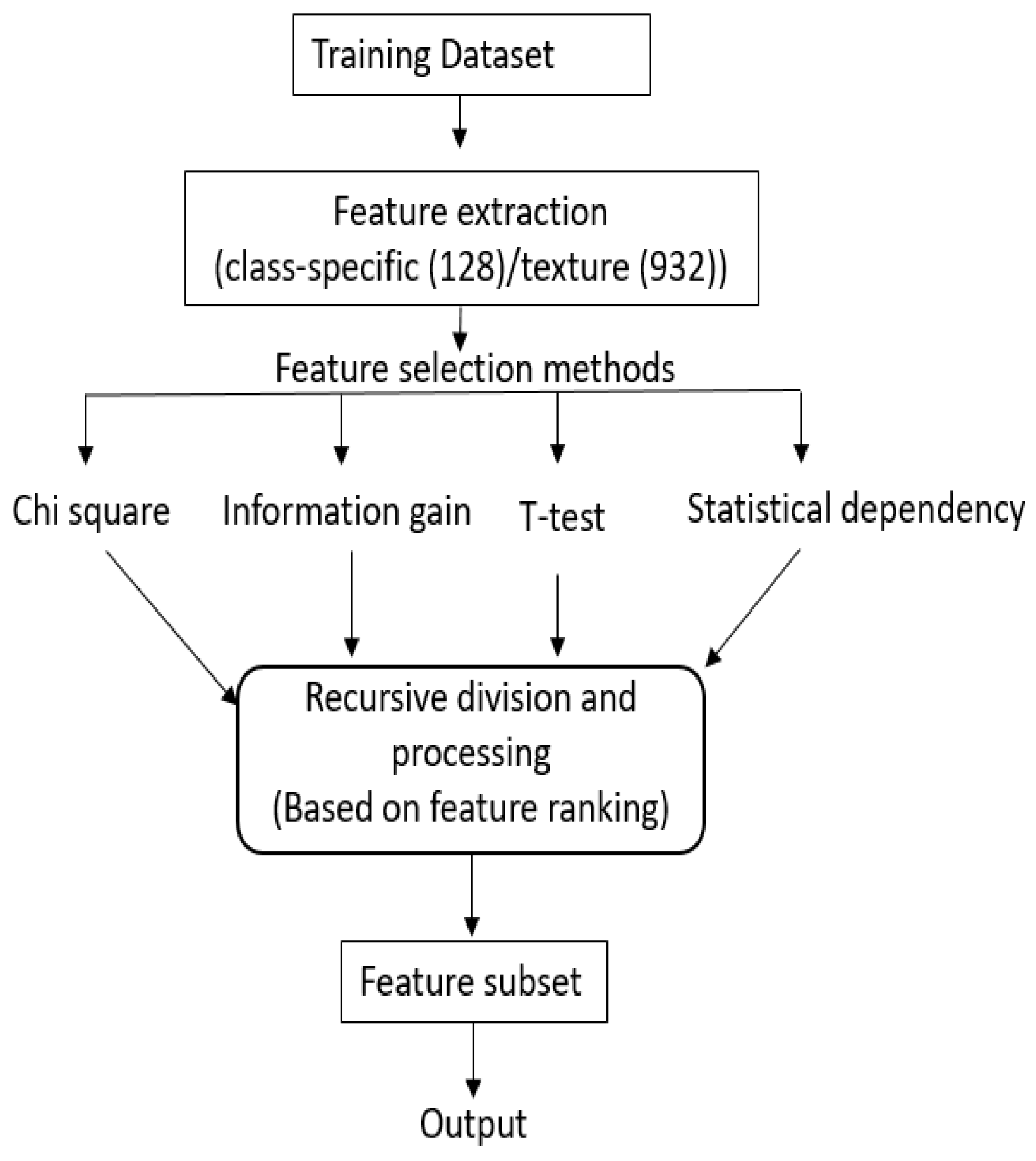
3. Methodology

We divide this subsection into four parts in which we discuss the details of the filter, wrapper, embedded, and unsupervised methods that we consider for feature selection.

3.1. Filter Methods and Their Hybridization

This subsection discusses about the four filter methods chosen for this work, and the proposed hybridization approach in detail. Figure 2 shows the architecture of proposed scheme.

3.1.1. Filter Methods

Filter techniques assess the relevance of features based on discriminative criteria. These are relatively independent of model performance, hence provide the score (feature ranking) by looking only at the intrinsic properties of the data. Chi square, t-test, information gain (IG) and statical dependency (SD) are some of the examples of filter methods.

• Chi square [17]: The chi-square test is a statistical test that is applied to test the independence of two variables. In context of feature selection, it is analogous to hypothesis testing on distribution of class labels (target) and feature value. The greater the chi-score of a feature, the more independent that feature is from the class variable.
• t-test: t-test is a statistical, hypothesis where the statistic follows a Student distribution. After calculating the score of t-Statistic for each feature, scores are sorted in descending order in order to rank the features. t-test is usually applied between two groups of data. As our problem consists multiple groups (multiple classes), there are two ways by which t-test can be carried out. (1) Multiple paired t-test (2) one-way ANOVA (one-way analysis of variance). In this work, we used ANOVA, which uses p-value and F-statistics. In this work, we rank the features based on the F-statistics.
• Information gain (IG) [49]: computes how much information a feature gives about the class label. Typically, it is estimated as the difference between the class entropy and the conditional entropy in the presence of the feature.

  $$I(C,A)=H\left(C\right)-H(C/A)$$

  (1)

  where C is the class variable, A is the attribute variable, and H( ) is the entropy. Features with higher IG score are ranked higher than features with lower scores.
• Statistical dependency (SD) [47]: measures the dependency between the features and their associated class labels. The larger the dependency, higher will be the feature score.

The involved filter methods are univariate i.e., each feature considered separately without involving any feature dependencies. These methods have various advantage over other methods: (1) can be easily scaled to high-dimensional datasets, (2) computationally simple and fast, (3) independent of the learning algorithm i.e., not specific to a given learning algorithm. Moreover, feature selection needs to be performed only once.

3.1.2. Hybridization Process

This subsection describes the hybridization process that involves various filters methods which provide feature ranking based on different criteria.

We believe that by hybridizing various filters methods, a feature set which has enough variation and yet is representative enough can be obtained automatically. Our proposed scheme of hybridization involves iterative choosing common features from the rank sorted sets by each of the filter methods. The procedure is described below:

• We recursively divide the sorted feature set from each of the N filter methods, into halves based on ranking. For example, if total features are 128, than we first process 64 top features, followed by 32, 16, …, 8, 4, 2, 1.
• Processing the first half: (1) An initial selected feature set contains features that are common in first half of rank-sorted features from all N methods, (2) We then keep adding to this list the common features from among first halves of the rank-sorted list of $N-1$ methods, if the addition improves the accuracy. We follow this process with $N-2$, $N-3$, …, 2 methods. Note that at each stage, we consider common features from all combinations of $N-1$, $N-2$, …, 2 methods.
• Processing lower partitions: The above process is then carried out for the lower partitions and sub-partitions, recursively. Note that as one proceeds lower in the partitions, the number of features added in the final feature sets reduce, as many do not contribute to the increase in the accuracy. At each evaluation the improvement in accuracy is computed with a training and validation set by training a support vector machines (SVM).

Figure 2 shows the architecture of Hybridization Process. The algorithm for this process are illustrated in Algorithm 1. We note that this is an effective way of selecting a ‘good’ feature set without manually setting empirical threshold on the rank to determine the number of features to be selected. Moreover, it also suggests an approach to integrate the ranking provided by different filter methods. As the proposed hybridization approach employs a validation based approach using a classifier, one can argue that it is similar to the wrapper FS method. However, the proposed method is different from a typical wrapper methods as: (1) It uses already ranked features to come across the final feature subset. Hence it requires much less number of iterations than wrapper methods which involve an exhaustive or random search considering individual features. (2) The wrapper methods stop adding features when it does not find increment in accuracy. Therefore, to proceed further there is a need to define a parameter which determines the number of features that can be allowed in the selected feature set without improvement.

To compare the proposed hybridization approach with the existing hybrid approaches, we implement the method [46] that was used for website phishing classification. In this method, the authors combine two filer methods (IG, chi-square). First they normalize both feature scores to make them comparable and, then calculate the root mean square of the feature values.

$$v_a=\sqrt{{\left(IG\right)}^2+{\left(Chi\right)}^2}$$

(2)

Algorithm 1 For finding feature subset using hybridization

1 Select F, common features from top half ranked features from N methods Repeat step a for every x=[N-1, N-2…2]         a) For all permutation of x,         choose common feature subset s                 for every feature f in s                         if D=(F union f) improves accuracy                                  keep                          Else                                  discard Output: set E 2 Take the lower half and find common subset of features SL         for every features t in SL                 if (E union t) improves accuracy                          keep                  Else                          discard Goto step 1 (a)

3.2. Wrapper Methods

Wrapper methods embed the model hypothesis (predictor performance) to find feature subsets. The space of feature subsets grows exponentially with the number of features, hence increase the overfitting risk.

• Sequential Forward Selection (SFS) [18]: It is an iterative method in which we start with an empty set. In each iteration, we keep adding the feature (one feature at a time) which best improves our model till an addition of a new variable does not improve the performance of the model. It is a greedy search algorithm, as it always excludes or includes the feature based of classification performance. The contribution of including or excluding a new feature is measured with respect to the set of previously chosen features using a hill climbing scheme in order to optimize the criterion function (classification performance).
• Random Subset Feature Selection (RSFS) [50]: In this method, in each step, random subset of features from all possible feature subset is chosen and estimated. The relevance of participating features keeps adjusting according to the model performance. As more iterations are performed, more relevant features obtain a higher score. and the quality of the feature set gradually improves. Unlike SFS, where the feature gain is estimated directly by excluding or including it from a existing set of features, in RSFS each feature is evaluated in terms of its average usefulness in the context of feature combinations. This method is not much susceptible to a locally optimal as SFS.

3.3. Embedded Methods and Feature Selection Procedure

In the following subsection we discuss about embedded methods considered in this work, viz. random forest and its variant, random uniform forest for measuring feature (variable) importance, and feature selection procedure which we employ in this work for both methods.

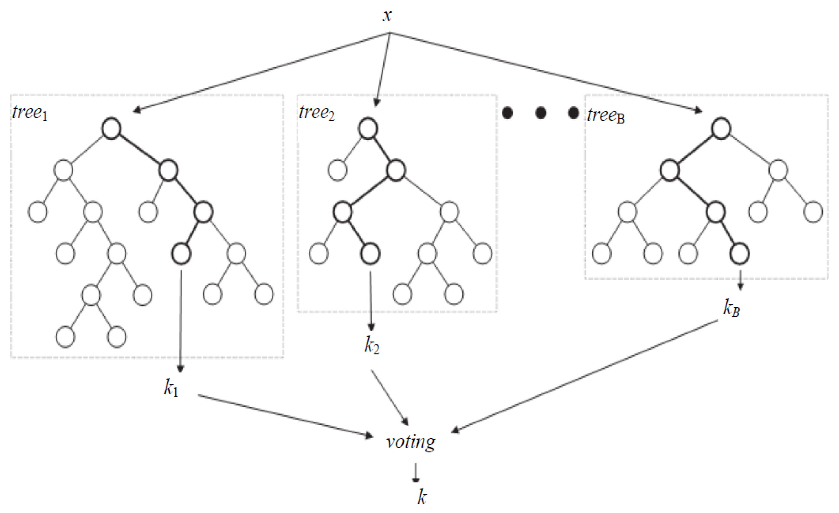
3.3.1. Random Forest

Random Forest [19] is a collection of decision trees where each tree is constructed using a different bootstrap sample from the original data. At each node of each tree, a random feature subset of fix size is chosen and the feature which yields maximum decrease in Gini index is chosen for split [19]. In the forest, trees are grown fully and left unpruned. About one-third of the samples, called out of bag samples (OOB), are the left out of the bootstrap sample and used as validation samples to estimate error rate. To predict the class of a new sample, votes received by each class are calculated and the class which has majority of the votes is assigned to the new sample. Figure 3 shows the general structure of random forest.

Random forest offers two different measures to gauge the importance of features, the variable importance ($VI$) and the Gini importance ($GI$) [19]. The average decrease in the model accuracy on the OOB samples when specific feature is randomly permuted gives the $VI$ of that feature. The random permutation essentially indicates the replacement of that feature with a randomly modified version of it. $VI$ shows how much the model fit decreases when we permute a variable. The greater the decrease the more significant is the variable. For variable $X_j$, the $VI$ is calculated as follows: (1) Calculate model accuracy without permutation using OOB samples, (2) Randomly permute the variable $X_j$, (3) Calculate model accuracy with permuted variable together with the remaining non-permuted variable, (4) Variable importance is found out by taking difference of accuracies before and after permutation and is averaged over all trees.

$$VI\left(X_j\right)={\displaystyle \frac{{\mathrm{\Sigma }}_{t=1}^{ntree}V{I}^t\left(X_j\right)}{ntree}}$$

(3)

Gini importance (GI) indicates the overall explanatory power of the variables. The $GI$ uses the drop in Gini index (impurity) as a measure of feature relevance. $GI$ is a biased estimate [51] when features vary in their scale of measurement. Owing to this $VI$ is more reliable for feature selection when subsampling without replacement is used instead of bootstrap sampling to construct the forest. Therefore, we consider the $VI$ measure for variable ranking in this paper.

3.3.2. Random Uniform Forest (RUF)

RUF is an ensemble of random uniform decision trees, which are unpruned and binary random decision trees. The random cut-points in an RUF, to create partition from each node, is generated assuming an uniform distribution for each candidate variable.

An important purpose of the algorithm is to get tress which are less correlated, to allow a better analysis of variable importance. For more details, please refer to [24].

RUF also provides a measure for variable importance as RF for assessment of features. However, in this case, the procedure of its estimation is decomposed into two steps: (1) first is same as RF, where VI is computed for all features, (2) In second step, relative influence of each feature is calculated. Thus, it is termed as global variable importance measure. Each variable has equal chance to be selected but it will get importance only if it is the one that decreases the overall entropy at each node. We rank the features based considering the variable importance from RF and RUF. We then provide an examination how overall accuracy varies when sets of top-ranked features are chosen and how many features are actually required to achieve accuracy equal (or in some cases, even greater) to accuracy which had been obtained with all features. In the result section, we will briefly discuss about the impact of top-ranked features on accuracy using two different feature sets.

3.3.3. Feature Selection Procedure

This subsection describes the procedure which we employ to seek a subset of features based on the variable importance. Same procedure is followed for both RF and RUF.

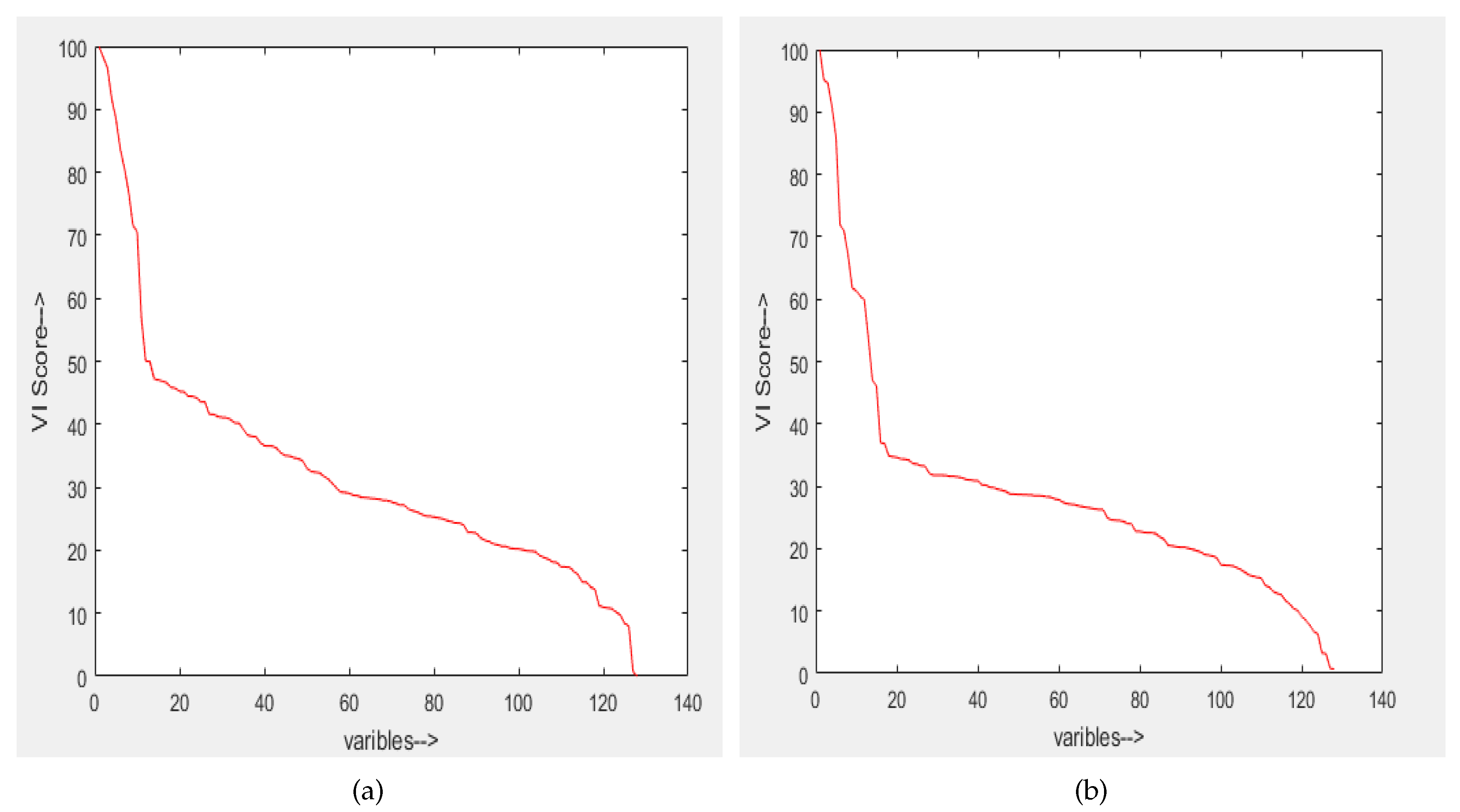
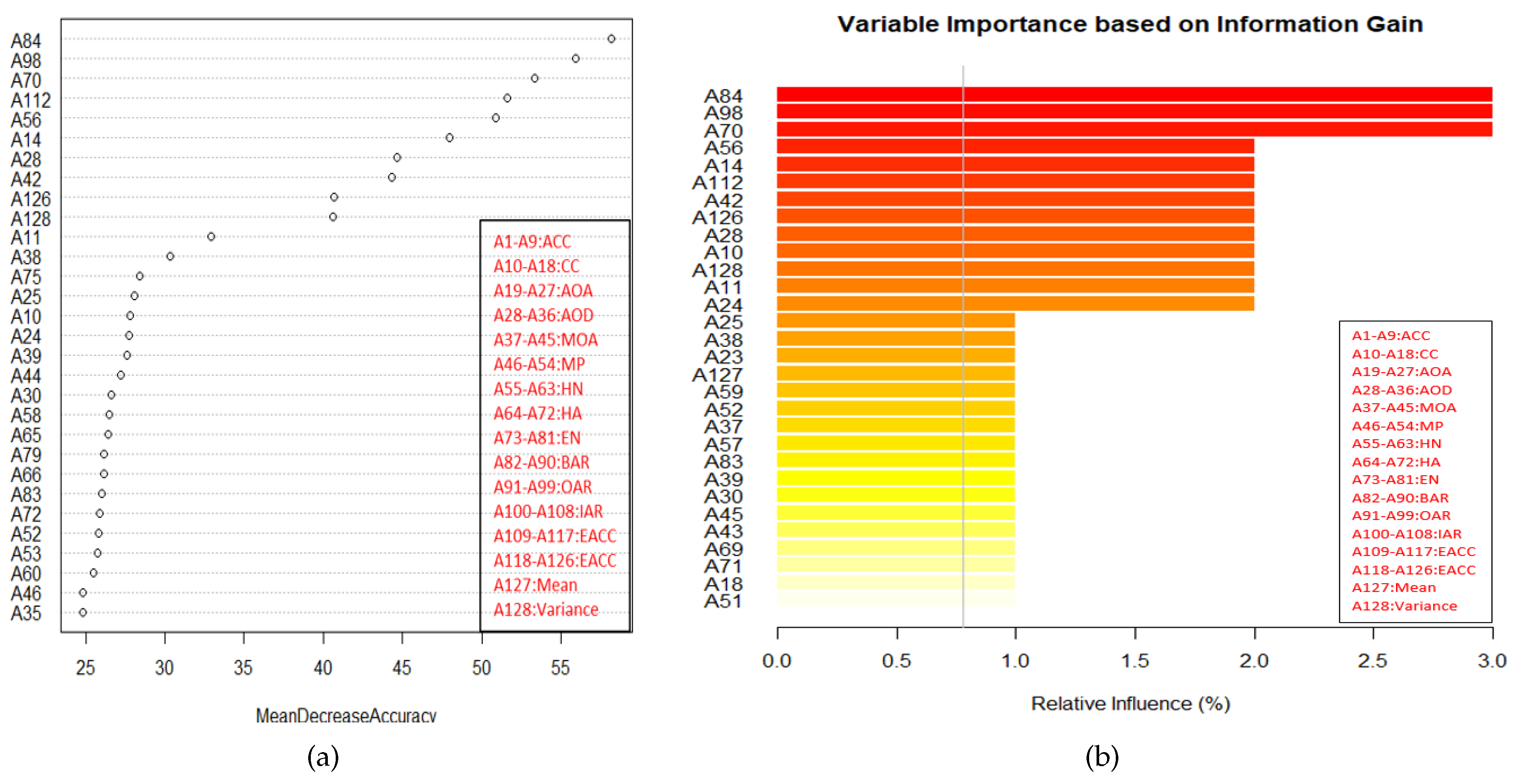
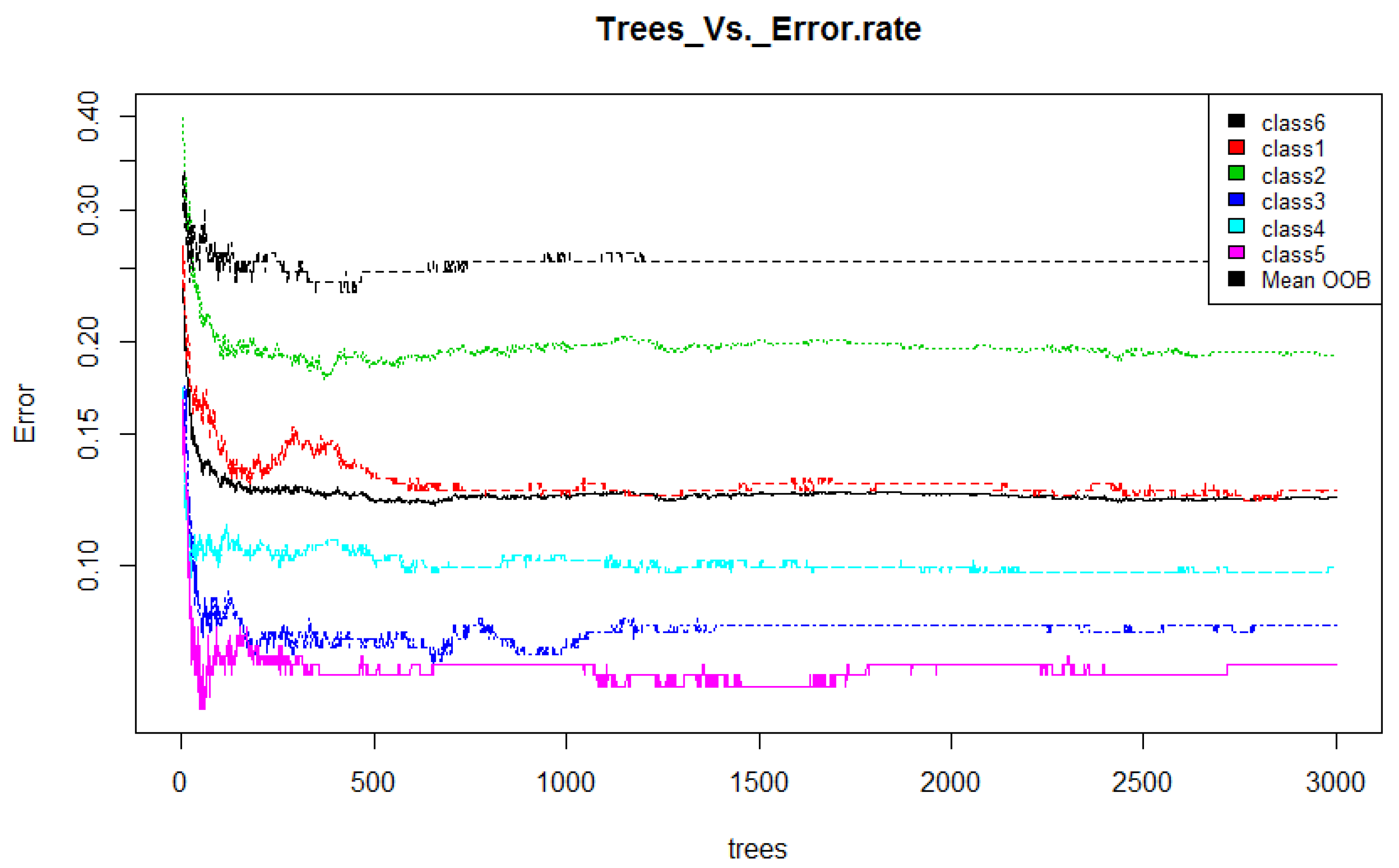
• Training: Random forest (RF) internally divides the training data into 67–33% ratio for each tree randomly, where 67% is used to train a model while 33% (out of bag) used for testing (cross-validation). The OOB error rate is calculated using this 33% data only. To automatically decide the value of RF parameters such as number of trees and number of features used at each tree, the OOB error rate is generally considered [52]. In this work, we only decide the number of trees. For the number of features at each tree, we employ typical default value (viz. square root of the total number of features). Figure 4 illustrates the variation in OOB error rate with the variation in the number of trees. There are seven lines in graph where six correspond to each class and the black line corresponds to mean of OOB error rate of all class. The point where the OOB error reduces negligibly could be considered as a good point to fix the value of number of trees [52].
• Feature selection: By using variable importance (VI) provided by RF (after cross-validation), a subset of good features is chosen to test the remaining 30% data. The procedure of selecting a good feature subset is given as follows:

  (a)

  Top ranked features (in terms of $VI$) in sets of 10 (e.g., 10, 20, 30, …) are used for testing.

  (b)

  After some point, addition of more features do not increase the classification accuracy further.

  (c)

  As there is no significant improvement after this point, the features upto this point is considered as good feature subset. This feature subset gives the accuracy which is equal to the accuracy obtained using all features.

3.4. Unsupervised Feature Selection

• Infinite Feature Selection (InFS) [20]: It is graph-based method. Each feature is a node in the graph, a path is a selection of features, and the higher the centrality score, the most important (or most different) the feature.
• Regularized Discriminative Feature Selection (UDFS) [21]: It is a L2,1-norm regularized discriminative feature selection method which simultaneously exploits discriminative information and feature correlations. It selects most discriminative feature subset from the whole feature set in batch mode.
• Multi Cluster feature selection (MCFS) [22]: It selects the features for those e multi-cluster structure of the data can be best preserved. Having used, spectral analysis it suggests a way to measure the correlations between different features without label information. Hence, it can well handle the data with multiple cluster structure.

4. Dataset and Feature Extraction

This subsection discusses the dataset used in this work and features we employ for the study. Indeed, one type of features that we employ is closely related to the visual traits of cell organelles observed in the images.

4.1. Dataset

In this work, the publicly available dataset from the ICPR 2014 HEp-2 cell image classification contest is used which comprising more than 13,000 cell images [7].

The dataset consist of six classes termed as: Homogeneous (H), Speckled (S), Nucleolar (N), Centromere (C), Nuclear Membrane (NM), Golgi (G). In the dataset, each class consist of positive and intermediate images. The intermediate images are generally lower in contrast compared to the positive images. The dataset also includes mask images which specify the region of interest of each cell image. Figure 5 provides the details of examples for each class.

4.2. Feature Extraction

One of our intentions in this work is to demonstrate that even simplistic feature definitions (unlike the more sophisticated ones such as SIFT, HOG, SURF etc.), can also yield good classification performance. Thus, we define two types of features. The first type which we term as ‘class-specific features’, are proposed in one of our earlier works [13], wherein we explicitly represent some semantic morphological aspects in the cell. For the second type of features, we choose some standard texture descriptors, but which yield only scalar values, thus are quite simplistic.

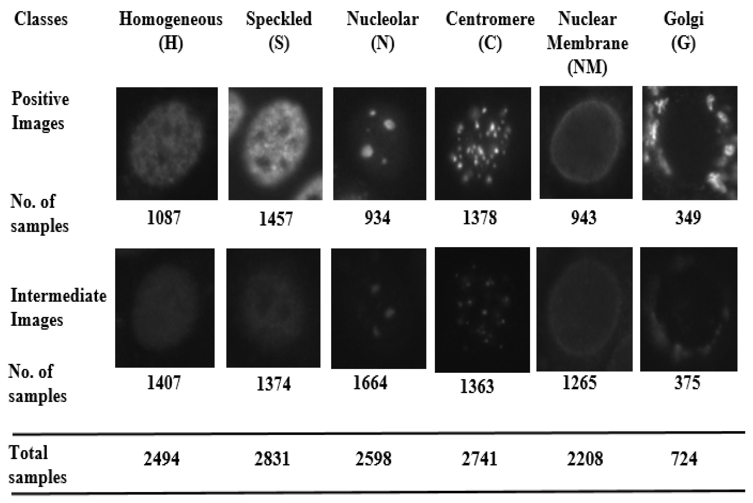
• Class-specific features: Motivated by expert knowledge [9] which characterizes each class by giving some unique morphological traits, we define features based on such traits. As the location of these traits in each class may be different, features are extracted from specific regions of interest (ROI) for each particular class, computed using the mask images. Figure 6 shows some of the unique traits of each class. For example, in NM class useful information can be found in a ring which is centered on the boundary. Thus, utilizing such visually observed traits following features are extracted for the NM class:

  1

  Boundary area ratio (BAR): It is a area ratio in boundary ring mask.

  2

  Inner area ratio (IAR): It is a area ratio in inner mask.

  3

  Eroded area connected component (EACC): It gives the number of white pixels in inner mask.

  Similarly, for the Centromere class the class specific features defined are:

  1

  Maximum object Area (MOA): Area of object having a maximum size.

  2

  Average object Area (AOA): Average area of objects.

  3

  Connected Component (CC): Total number of objects in the cell.

  Here we only mention a list of these features in

  Table 1. Class-specific features for all classes.

  Classes	Class-Specific Features
  Homogeneous	Maximum object area (MOA), Area of connected component (ACC), Maximum perimeter (MP)
  Speckled	Hole area (HA), Hole number (HN), Euler number (EN)
  Nuleolar	Maximum object area (MOA), Average object area (AOA), Connected component (CC)
  Centromere	Maximum object area (MOA), Average object area (AOA), Connected component (CC)
  Nuclear Membrane	Boundary area ratio (BAR), Inner area ratio (IAR), Eroded area connected component (EACC)
  Golgi	Outer area ratio (OAR), Average object distance (AOD), Eroded area, connected component (EACC)

  , but and we refer the reader to our previous work [13] which contains a more elaborate discussion. These features, involve simple image processing operations such as scaler image enhancement, thresholding, connected components. and morphological operation. Our earlier work [13] explains the features in more detail. These feature are scalar-valued, simple, efficient, and more interpretable. As listed in Table 1, the total feature definitions which are extracted from all classes is 18, and using various combination of threshold and enhancement parameters, a total 128 features are obtained.
• Traditional scalar texture features [14]: These include features which include morphology descriptors (like Number of objects, Area, Area of the convex hull, Eccentricity, Euler number, Perimeter), and texture descriptors (e.g., Intensity, Standard deviation, Entropy, Range, GLCM) are extracted at 20 intensity thresholds equally spaced from its minimum to its maximum intensity. Again for a detailed description about these features, one can refer [14]. However, in [14], these features were applied on much smaller dataset. Considering various parameter variations, in this case, a much larger set of 932 scalar-valued features is obtained.

5. Results and Discussion

In this section we discuss the experimental protocols and results, comparing among the different FS methods, and finally provide a comparison with the state-of-the-art approaches.

5.1. Training and Testing Protocols

In this section we discuss the experimental results obtained using the two different feature sets discussed above. We divide the given data into three parts: training (40%), validation (30%) and testing (30%) (Experimental protocol 1). All the experiments are done for four random trails, and average accuracies are reported for all. The state-of-the-art methods differ in their experimentation protocol. Hence, here, we also consider an experimental setup in which training, validation and testing ratios are defined in the same manner as the methods that yield the highest performance. This is a 5-fold cross-validation protocol where the training-validation data consists of 80% portion and the test data is 20% [Experimental protocol 2]. Note that the protocol 1 involves lesser training data than the best performing approaches (protocol 2). We first provide and discuss with protocol 1 for all the approaches, before providing results for protocol 2. esting (80%). This is motivated by the fact that in realistic applications the amount of training data is low.

5.2. Evaluation Metrics

Various metrics can be utilized to evaluate performance. In the paper [7] which is associated with the dataset used in this work, mean class accuracy (MCA) was used to evaluate the performance. Here, we utilize mean class accuracy, and in addition we also employ overall accuracy and false positive as evaluation measures for fair comparison with other state-of-art methods [11,30,31,32,33,34] which also use the same metrics.

$$MCA=\sum _{i=1}^N\frac{CC\left(i\right)}{N_i}$$

(4)

where $CC\left(i\right)$, $N_i$ are the classification accuracy and total samples of class i, and N is the total number of classes (here it is 6).

False Positive ($FP$): It is a proportion of negatives samples that are incorrectly classified as positive.

$$FP=1/N\sum _{i=1}^N{\displaystyle \frac{WC\left(i\right)}{F{S}_i}}$$

(5)

where $WC\left(i\right)$ is the wrongly classification samples of class i and $F{S}_i$ is the false samples for class i (for example, for class 1, the samples of other classes (2, 3, 4, 5 and 6) will be the false samples).

The overall accuracy ($OA$), which is the overall correct classification rate is also calculated for ease of comparison, is given as:

$$OA=1/N\sum _{i=1}^{N}CC\left(i\right)$$

(6)

To follow below tables, notions $A_h$, $N_h$, $A_s$ and $N_s$ are defined as:

• $A_h$: Highest accuracy with respect to the number of selected features.
• $N_h$: Number of features that yield the highest accuracy.
• $A_s$: Accuracy considering all features.
• $N_s$: Number of features that match the accuracy considering all features.

Each table provides the exact number for $N_h$, $N_s$ and for their corresponding $A_h$, $A_s$ for four random trails. From tables, it is clear that highest accuracy is slightly higher than accuracy obtained using all features. The reason is that including features which are not important, or correlated features can negatively impact the accuracy. In all the tables, an average value of Ah, Nh, As, Ns is reported across four random trails.

5.3. Results: Protocol 1

5.3.1. Filter Methods

For each filter method, the following procedure is opted to choose feature subset which produces higher accuracy using the obtained feature ranking: (1) Features are tested on validation data in sets of 1 (e.g., 1, 2, 3, 4, …). We utilize support vector machine (SVM) with gaussian kernel for classification. (2) After some point, addition of more features do not increase the classification accuracy further. Although, in some cases it also decreases up to some point.

Table 2. Filter methods: Experimental protocol 1.

Class-Specific Features (Total Features: 128)						Texture Features (Total Features: 932)
Methods/Trials		Chi Square	t-Test	Information Gain	Statistical Dependency	Chi Square	t-Test	Information Gain	Statistical Dependency
Average (Validation)	Ah	98.43	98.47	97.98	98.43	95.14	94.97	95.14	94.93
	Nh	98	98	93	98	756	812	702	863
	As	98.23	98.12	97.57	98.23	94.72	94.72	94.73	94.72
	Ns	91	85	84	91	730	693	666	838
Testing	Ah	98.16	98.16	97.44	98.23	94.74	94.50	95.05	94.26
Testing	As	98.10	97.41	97.03	98.13	94.35	94.17	95.00	94.20

describes the results obtained from filter methods using both datasets. Following observation can be made: (1) These methods select more features or are able to reject relatively few features. This happens, because interaction among features (relative importance) are not considered in process of making feature ranking. Approximately 75% features of class-specific set, and 84% features of texture set are utilized for the highest accuracy, whereas 68% features of class-specific set, and 78% texture features are used to match the performance same as using all features. (2) Although, these methods select larger number of features, they can better be generalize to unseen data i.e., the case where distribution of output data is somewhat different from input data. This can be seen through the small difference between validation and testing results.

5.3.2. Hybridization

The results of proposed hybridization strategy of the filter methods are given in

Table 3. Hybridization results: Experimental protocol 1.

Hybridization
	Class-Specific Features (Total Features: 128)				Texture Features (Total Features: 932)
	Trail 1	Trail 2	Trail 3	Trail 4	Trail 1	Trail 2	Trail 3	Trail 4
Ah	98.33	98.65	97.98	98.62	95.09	95.48	95.31	95.90
Nh	86	91	85	95	521	536	546	585
As	98.33	98.65	97.98	98.62	95.04	95.31	95.31	95.90
Ns	86	91	85	95	478	520	546	585
Average Results (Validation)
Ah	98.39				95.45
Nh	89				547
As	98.39				95.39
Ns	89				532
Testing
Ah	98.28				94.90
As	98.28				94.90

and shown for four random trials. It can be noticed from the table that the hybridization produces highest accuracy (among all methods, especially with class-specific features), but with less number of selected features than its component filter methods. However, the selected feature subset still contains features which are more than wrapper and embedded methods (to be discussed next). Nevertheless, it also produces the highest testing accuracy with both datasets.

An important point is that the increment in the size of feature set during the selection process can be controlled in wrapper and embedded methods (for features can be added one by one), while in hybridization method, this is automatic, and a large chunk of features (which are common across the high-ranked filter methods) is selected simultaneously. This could be the one of reason to get high length feature subset.

5.3.3. Wrapper Methods

Table 4. Wrapper and embedded methods: Experimental protocol 1.

Class-Specific Features (Total Features: 128)						Texture Features (Total Features: 932)
Methods		Wrapper		Embedded		Wrapper		Embedded
		SFS	RSFS	RF	RUF	SFS	RSFS	RF	RUF
Average (Validation)	Ah	98.17	96.92	97.44	97.78	90.57	94.44	94.29	95.25
	Nh	87	30	66	60	35	133	202	258
	As	-	-	97.22	97.66	-	-	93.75	94.87
	Ns	-	-	41	32	-	-	60	154
Testing	Ah	97.88	96.78	97.19	97.55	88.14	90.62	94.18	95.13
Testing	As	-	-	97.13	97.36	-	-	93.60	94.84

illustrates the results for wrapper methods. Following inferences can be made through observations: (1) It considers the relative importance of features while making optimal subset. Hence the feature which has higher individual, as well as relative importance will be chosen first. This method calculates the importance of each feature with respect to other features. As, this method selects features till it finds an increment in performance, it can sometimes get trapped in local minima. However, it can be observed from the table that, this approach selects least features (<15%) as compared to others, to generate high accuracy. However, the difference between validation and testing accuracy shows that it may not be able to better generalize to new samples (unseen data), as sometimes it over-fit to the training data, even based on the parameters chosen with the validation data.

5.3.4. Embedded Methods

To determine the effectiveness of random forest and random uniform forest, for feature importance the experiment involves two steps: (1) Computing the variable importance ($VI$) of features, (2) Computing the classification performance using top ranked features (in sets of 10). The same procedure is repeated for four random trials. The testing and validation results shows that embedded methods can be better generalize to unseen data than wrapper method even with less number of features. We note that (Table 4) only 25–35% features are sufficient to yield accuracy which is equal to standard accuracy (i.e., using all features) for the class-specific feature set, while for the texture feature set, approx <20% features are sufficient for the same. Thus, as in the wrapper methods the number of feature selected are quite low. Figure 7 shows the ranking of feature based on the variable importance, given by random forest and random uniform forest for one of the feature set (class-specific: one trial). The variable importance along with variable name are shown in Figure 8. Figure 8a shows the decease in accuracy when randomly permute the variable for Random forest, Figure 8b shows the relative influence of variables for Random uniform forest.

5.3.5. Unsupervised Feature Selection Methods

The results for unsupervised FS methods are given in

Table 5. Unsupervised features selection methods: Experimental protocol 1.

	Class-Specific (128)			Texture (932)
Average	MCFS	InFS	UDFS	MCFS	InFS	UDFS
Ah	98.35	98.06	98.15	94.88	94.81	94.80
Nh	108	118	99	918	811	853
As	98.03	98.03	93.03	90.39	90.20	89.26
Ns	91	115	89	321	323	291
Testing (Ah)	98.17	97.95	98.10	94.75	94.69	94.60
Testing (As)	97.94	97.94	98.05	90.63	89.69	89.27

. Following can be observed from Table 5: (1) It produces validation accuracy which is somewhat lesser than supervised (filter methods). But Produces higher test accuracy. (2) Required more number of features than supervised domain methods.

5.4. Results: Protocol 2

From the results obtained using protocol 1, it can be seen that higher accuracies are produces with filter, embedded, hybrid and unsupervised methods. Due to this, we only implement such methods for second protocol.

Table 6. Filter and hybrid methods: Experimental protocol 2.

	Class-Specific features (Total Features: 128)
	Filter Methods					Embedded
Average	Chi Square	t-Test	IG	SD	Hybrid	RF	RUF
Ah	98.73	98.73	98.72	98.65	98.65	97.51	97.87
Nh	95	113	108	118	85	66	54
As	98.64	98.62	98.62	98.62	98.65	97.32	97.77
Ns	86	105	97	118	85	40	38
Testing (Ah)	98.66	98.49	98.51	98.54	98.59	97.51	97.78
Testing (As)	98.51	98.10	98.42	98.40	98.59	97.26	97.60
Texture Features (Total Features: 932)
Ah	95.82	96.61	95.83	95.95	95.90	94.67	94.93
Nh	810	847	750	791	465	250	330
As	95.47	95.47	95.47	95.47	95.90	93.89	94.60
Ns	742	798	465	675	465	80	120
Testing (Ah)	96.00	95.76	95.51	96.00	95.51	94.21	95.11
Testing (As)	95.92	95.71	95.51	95.91	95.51	93.01	94.91

describes the results for filter and hybrid methods using both datasets. As protocol 2 uses more training data, it produces higher accuracy than protocol 1. However, it also utilizes more features. Other observation are same as above. Results for unsupervised methods are shown in

Table 7. Unsupervised features selection methods: Experimental protocol 2.

	Class-Specific (128)			Texture (932)
Average	MCFS	InFS	UDFS	MCFS	InFS	UDFS
Ah	98.80	98.67	98.71	95.70	95.58	95.60
Nh	97	116	117	905	797	816
As	98.62	98.62	98.61	90.16	90.55	89.95
Ns	90	113	121	284	280	284
Testing (Ah)	98.66	98.49	98.46	95.77	95.83	95.78
Testing (As)	98.63	98.21	98.32	90.34	90.75	90.26

.

5.5. Comparison among All Feature Selection Methods

Table 8. Comparison of methods: Experimental protocol 1.

Class-Specific Features (Total Features: 128)
	Filter					Wrapper		Embeded
Average	Chi Square	t-Test	Information Gain	Statistical Dependency	Hybrid	SFS	RSFS	RF	RUF
Ah	98.43	98.47	97.98	98.43	98.39	98.17	96.92	97.44	97.78
Nh	98	98	93	98	89	87	30	66	60
As	97.57	98.12	98.23	98.03	98.39	-	-	97.22	97.66
Ns	91	85	84	91	89	-	-	41	32
Testing (Ah)	98.16	98.16	97.44	98.23	98.28	97.88	96.78	97.19	97.55
Testing (As)	98.10	97.41	97.03	98.13	98.28	97.88	96.78	97.13	97.36
Texture Features (Total Features: 932)
Ah	95.14	94.97	95.14	94.93	95.45	90.57	94.44	94.29	95.25
Nh	756	812	702	863	547	35	133	202	258
As	94.72	94.72	94.73	94.72	95.39	-	-	93.75	94.87
Ns	730	693	666	838	532	-	-	60	154
Testing (Ah)	94.74	94.50	95.05	94.26	94.90	88.14	90.62	94.18	95.13
Testing (As)	94.35	94.06	95.00	94.20	94.90	88.14	90.62	93.60	94.84

provides comparable performance among all the feature selection methods under one roof for protocol 1. From this, and from Table 2, Table 3 and Table 4, it can be observed that (1) Filters methods have better generalization ability than other methods which involve the classification performance, at the cost of optimal subset that contains large number of features compared to other methods. Hence, they performs well on unseen data. (2) Since filter methods selects larger dimension of feature subset, the cases where number of sample are less than number of features (for example, for bio-informatic applications [42,53]), wrapper methods typically perform well as compared to filter methods. (3) Hybridization of filters methods produces better performance than individual filter methods. It also selects less number of features compared to individual filter methods. (4) In can be seen that, in general for class-specific features, there is relatively less difference in number of optimal features selected across all methods. This indicates that the class-specific features are designed thoughtfully based on semantic visual characteristics of the cell images, and hence there may not be too many irrelevant features. However, this difference in numbers of selected features is clearly seen in case of texture features. (5) Also, in general, the highest accuracy obtained using the class-specific features is also, higher than that of texture features. (6) Both wrapper and embedded methods yield a high accuracy, importantly with less number of features. However, for the texture feature set, one can note that the generalization capability of the wrapper methods is low, as there is a considerable difference between the validation and the testing accuracy. (7) In general, considering overall testing accuracy and the number of features selected, the embedded methods can be said to perform best. However, if the computational complexity (i.e., the number of selected features) is not much of a concern, then the hybridization of filter methods yields the best results.

As we are reporting all the results corresponding to both the protocols in comparison section (with contemporary methods). Due to this reason, we are not adding table for protocol 2.

5.6. Performance Comparison with Contemporary Methods

Table 9. Performance comparison.

Methods	Experimental-Setup	Metrics Evaluation			Nh (Number of Features)
		MCA (%)	FP (%)	OA (%)
Prasath et al. [30]	5-fold cross-validation (Training: 80%, Testing: 20%)	94.29	NA	NA	552
Bran et al. [31]	5-fold cross-validation (Training: 64%, validation: 16%, Testing: 20%)	89.79	10.33	90.59	NA
Praful et al. [32]	10-fold cross-validation	NA	NA	92.85 ± 0.63	211
Shahab et al. [11]	7-fold cross-validation	94.9	5.09	94.48	NA
Siyamalan et al. [33]	2-fold cross-validation (each repeated 10 times)	92.58 (95.21)	7.38 (4.8)	NA	NA
Zhimin et al. [34]	Data-augmentation (Training: 64%, validation: 16%, Testing: 20%)	88.58 (96.76)	NA	89.04 (97.24)	NA
Supervised Feature Selection
Proposed (Filter: Chi): class-specific	5-fold cross-validation (Training: 64%, validation: 16%, Testing: 20%)	98.62 ± 0.37	1.70 ± 0.56	98.66 ± 0.30	95
Proposed (Embedded: RUF): class-specific	5-fold cross-validation (Training: 64%, validation: 16%, Testing: 20%)	97.46 ± 0.55	0.49 ± 0.06	97.73 ± 0.32	54
Proposed (Filter: Chi): Texture	5-fold cross-validation (Training: 64%, validation: 16%, Testing: 20%)	95.23 ± 0.81	4.19 ± 0.74	96.00 ± 0.52	810
Proposed (Embedded: RUF): Texture	5-fold cross-validation (Training: 64%, validation: 16%, Testing: 20%)	93.92 ± 0.92	1.09 ± 0.12	95.11 ± 0.55	330
Proposed (Filter: SD): class-specific	Training: 40%, validation: 30%, Testing: 30% Repeated for four random trails	98.12 ± 0.32	2.19 ± 0.55	98.23 ± 0.38	98
Proposed (Wrapper: SFS): class-specific	Training: 40%, validation: 30%, Testing: 30% Repeated for four random trails	97.88 ± 0.39	2.44 ± 0.22	97.73 ± 0.37	87
Proposed (Embedded: RUF): class-specific	Training: 40%, validation: 30%, Testing: 30% Repeated for four random trails	97.55±0.52	0.51 ± 0.07	97.36 ± 0.45	60
Proposed (Filter: IG): Texture	Training: 40%, validation: 30%, Testing: 30% Repeated for four random trails	93.79 ± 0.23	5.66 ± 0.61	95.05 ± 0.43	702
Proposed (Wrapper: RSFS): Texture	Training: 40%, validation: 30%, Testing: 30% Repeated for four random trails	90.62 ± 0.55	9.74 ± 0.56	89.15 ± 0.34	133
Proposed (Embedded: RUF): Texture	Training: 40%, validation: 30%, Testing: 30% Repeated for four random trails	95.13 ± 0.67	1.06 ± 0.17	94.06 ± 0.81	258
Unsupervised Feature Selection
Proposed: Class-specific	5-fold cross-validation (Training: 64%, validation: 16%, Testing: 20%)	98.62 ± 0.22	1.67 ± 0.53	98.66 ± 0.32	97
Proposed: Texture	5-fold cross-validation (Training: 64%, validation: 16%, Testing: 20%)	94.95 ± 0.41	4.39 ± 0.68	95.83 ± 0.74	905
Proposed: Class-specific	Training: 40%, validation: 30%, Testing: 30% Repeated for four random trails	97.88 ± 0.18	2.18 ± 0.53	98.14 ± 0.18	108
Proposed: Texture	Training: 40%, validation: 30%, Testing: 30% Repeated for four random trails	93.29 ± 0.32	5.90 ± 0.16	94.75 ± 0.07	914
Hybridization
Proposed (hybrid): class-specific	5-fold cross-validation (Training: 64%, validation: 16%, Testing: 20%)	98.48 ± 0.35	1.78 ± 0.67	98.59 ± 0.31	85
Hybrid (exist): class-specific	5-fold cross-validation (Training: 64%, validation: 16%, Testing: 20%)	98.59 ± 0.38	1.68 ± 0.56	98.65 ± 0.30	99
Proposed (hybrid): Texture	5-fold cross-validation (Training: 64%, validation: 16%, Testing: 20%)	94.72 ± 1.04	4.70 ± 0.77	95.51 ± 0.54	465
Hybrid (exist): Texture	5-fold cross-validation (Training: 64%, validation: 16%, Testing: 20%)	95.11 ± 0.70	4.29 ± 0.42	95.90 ± 0.71	819
Proposed (hybrid): class-specific	Training-40%, validation-30%, Testing-30% Repeated for four random trails	98.15 ± 0.48	2.09 ± 0.43	98.23 ± 0.23	89
Hybrid (exist): class-specific	Training: 40%, validation: 30%, Testing: 30% Repeated for four random trails	98.21 ± 0.32	2.10 ± 0.57	98.29 ± 0.29	94
Proposed (hybrid): Texture	Training: 40%, validation: 30%, Testing: 30% Repeated for four random trails	93.84 ± 0.76	5.44 ± 0.34	94..90 ± 0.43	547
Hybrid (exist): Texture	Training: 40%, validation: 30%, Testing: 30% Repeated for four random trails	93.61 ± 0.58	5.49 ± 0.30	95.07 ± 0.45	737

illustrates the performance comparison (using both the protocols) among various methods, where in [30,31,32] utilized random forest for classification, [11,33] are recent methods using, arguably, more sophisticated features, and the work of [34] uses deep learning. For the methods in [33,34], the numbers in brackets denote the results with data augmentation.

In this table, for our approaches, we report the average results over 4 trials corresponding to Nh (Number of features that yield the highest accuracy). The results are shown only for one FS method out of many, in each category that produces higher accuracy.

From the table, following can be observed: (1) Considering the best results, the proposed approach where class-specific features are utilized, outperforms all the methods in all terms (overall accuracy, mean accuracy and false positives). (2) All types of feature selection methods used with class-specific features outperforms the state-of-art methods. (3) Even with the texture features, comparable performance is achieved for the hybrid filter method and the embedded methods.

Experimental protocol 1 where less training data as compared to protocol 2 is used, produces comparable performance with less number features. It could be considered as a positive aspect of our approach, such that using less training data higher performance can be obtained.

Thus, it is clear that many of the proposed approaches outperforms the other contemporary methods even with simple morphology-based and texture features. Importantly, often times, very less number of features are utilized.

5.7. Computational Time Analysis

We have not done an extensive computational time analysis, as different methods may use different platforms. However, we can speculate that during the testing process, the proposed approaches would arguably be more efficient, as it involves less number of features as compared to other methods, and efficient classifier, especially, as compared to the approach based on CNN classifier. Having said that, during the training and feature selection stage, we also note that the complexity of methods can vary based various factors. For example, in case of Random Forests, large number of trees may require more time as compared to less number of trees.

6. Conclusions

This work explored various feature selection methods from the perspective of HEp-2 cell classification. We also proposed a technique which combines filters methods. We showed that by constructing hybrid feature selection techniques, robustness of feature ranking and feature subset selection could be improved automatically.

We explore random forest and random uniform forest for feature selection for HEp-2 cell image classification. The notion of variable importance is used to select important features from a large set of simple features. Our experiments show that such a feature selection yields a significantly reduced feature subset, which can, in fact, result in accuracy higher than that using original large feature set. For comparison, we also employ some wrapper methods. The method also generalizes well for unseen data with a high performance with the reduced feature set.

The results demonstrate, in some cases, reduction of large feature set for the best performance on the test data, indicating potential computational saving. Also, in general the approach with proposed class-specific features outperforms the state-of-art methods.

References

- Sack, U.; Conrad, K.; Csernok, E.; Frank, I.; Hiepe, F.; Krieger, T.; Kromminga, A.; Von Landenberg, P.; Messer, G.; Witte, T.; et al. Autoantibody Detection Using Indirect Immunofluorescence on HEp-2 Cells. Ann. N. Y. Acad. Sci. 2009, 1173, 166–173. [Google Scholar] [CrossRef] [PubMed]
- Friou, G.J.; Finch, S.C.; Detre, K.D.; Santarsiero, C. Interaction of nuclei and globulin from lupus erythematosis serum demonstrated with fluorescent antibody. J. Immunol. 1958, 80, 324–329. [Google Scholar] [PubMed]
- Foggia, P.; Percannella, G.; Soda, P.; Vento, M. Benchmarking HEp-2 cells classification methods. IEEE Trans. Med. Imaging 2013, 32, 1878–1889. [Google Scholar] [CrossRef] [PubMed]
- Wiik, A.S.; Høier-Madsen, M.; Forslid, J.; Charles, P.; Meyrowitsch, J. Antinuclear antibodies: A contemporary nomenclature using HEp-2 cells. J. Autoimmun. 2010, 35, 276–290. [Google Scholar] [CrossRef] [PubMed]
- Kumar, Y.; Bhatia, A.; Minz, R.W. Antinuclear antibodies and their detection methods in diagnosis of connective tissue diseases: A journey revisited. Diagn. Pathol. 2009, 4, 1–10. [Google Scholar] [CrossRef] [PubMed]
- Hobson, P.; Lovell, B.C.; Percannella, G.; Vento, M.; Wiliem, A. Benchmarking human epithelial type 2 interphase cells classification methods on a very large dataset. Artif. Intell. Med. 2015, 65, 239–250. [Google Scholar] [CrossRef] [PubMed]
- Hobson, P.; Percannella, G.; Vento, M.; Wiliem, A. Competition on cells classification by fluorescent image analysis. In Proceedings of the 20th IEEE International Conference on Image Processing (ICIP), Melbourne, Australia, 15–18 September 2013; pp. 2–9. [Google Scholar]
- Bradwell, A.; Hughes, R.S.; Harden, E. Atlas of Hep-2 Patterns and Laboratory Techniques; Binding Site: Birmingham, UK, 1995. [Google Scholar]
- Foggia, P.; Percannella, G.; Soda, P.; Vento, M. Early experiences in mitotic cells recognition on HEp-2 slides. In Proceedings of the 2010 IEEE 23rd International Symposium on Computer-Based Medical Systems (CBMS), Perth, Australia, 12–15 October 2010; pp. 38–43. [Google Scholar]
- Iannello, G.; Percannella, G.; Soda, P.; Vento, M. Mitotic cells recognition in HEp-2 images. Pattern Recognit. Lett. 2014, 45, 136–144. [Google Scholar] [CrossRef]
- Ensafi, S.; Lu, S.; Kassim, A.A.; Tan, C.L. A bag of words based approach for classification of hep-2 cell images. In Proceedings of the 2014 1st Workshop on Pattern Recognition Techniques for Indirect Immunofluorescence Images (I3A), Stockholm, Sweden, 24 August 2014; pp. 29–32. [Google Scholar]
- Stoklasa, R.; Majtner, T.; Svoboda, D. Efficient k-NN based HEp-2 cells classifier. Pattern Recognit. 2014, 47, 2409–2418. [Google Scholar] [CrossRef]
- Gupta, V.; Gupta, K.; Bhavsar, A.; Sao, A.K. Hierarchical classification of HEp-2 cell images using class-specific features. In Proceedings of the European Workshop on Visual Information Processing (EUVIP 2016), Marseille, France, 25–27 October 2016. [Google Scholar]
- Strandmark, P.; Ulén, J.; Kahl, F. Hep-2 staining pattern classification. In Proceedings of the 2012 21st International Conference on Pattern Recognition (ICPR), Tsukuba, Japan, 11–15 November 2012; pp. 33–36. [Google Scholar]
- Blum, A.L.; Langley, P. Selection of relevant features and examples in machine learning. Artif. Intell. 1997, 97, 245–271. [Google Scholar] [CrossRef]
- Reunanen, J. Overfitting in making comparisons between variable selection methods. J. Mach. Learn. Res. 2003, 3, 1371–1382. [Google Scholar]
- Liu, H.; Setiono, R. Chi2: Feature selection and discretization of numeric attributes. In Proceedings of the Seventh International Conference on Tools with Artificial Intelligence, Herndon, VA, USA, 5–8 November 1995; pp. 388–391. [Google Scholar]
- Whitney, A.W. A direct method of nonparametric measurement selection. IEEE Trans. Comput. 1971, 100, 1100–1103. [Google Scholar] [CrossRef]
- Breiman, L. Random forests. Mach. Learn. 2001, 45, 5–32. [Google Scholar] [CrossRef]
- Roffo, G.; Melzi, S.; Cristani, M. Infinite Feature Selection. In Proceedings of the 2015 IEEE International Conference on Computer Vision (ICCV), Washington, DC, USA, 7–13 December 2015; pp. 4202–4210. [Google Scholar]
- Yang, Y.; Shen, H.T.; Ma, Z.; Huang, Z.; Zhou, X. L2,1-norm Regularized Discriminative Feature Selection for Unsupervised Learning. In Proceedings of the Twenty-Second International Joint Conference on Artificial Intelligence (IJCAI’11)—Volume Volume Two, Barcelona, Spain, 16–22 July 2011; pp. 1589–1594. [Google Scholar]
- Cai, D.; Zhang, C.; He, X. Unsupervised feature selection for multi-cluster data. In Proceedings of the 16th ACM SIGKDD International Conference on Knowledge Discovery and Data Mining, Washington, DC, USA, 24–28 July 2010; ACM: New York, NY, USA, 2010; pp. 333–342. [Google Scholar]
- Yang, Y.H.; Xiao, Y.; Segal, M.R. Identifying differentially expressed genes from microarray experiments via statistic synthesis. Bioinformatics 2004, 21, 1084–1093. [Google Scholar] [CrossRef] [PubMed]
- Ciss, S. Variable Importance in Random Uniform Forests. 2015. [Google Scholar]
- Gupta, V.; Bhavsar, A. Random Forest-Based Feature Importance for HEp-2 Cell Image Classification. In Proceedings of the Annual Conference on Medical Image Understanding and Analysis, dinburgh, UK, 11–13 July 2017; Communications in Computer and Information Science (CCIS). Springer: Cham, Switzerland, 2017; Volume 723, pp. 922–934. [Google Scholar]
- Perner, P.; Perner, H.; Müller, B. Mining knowledge for HEp-2 cell image classification. Artif. Intell. Med. 2002, 26, 161–173. [Google Scholar] [CrossRef]
- Huang, Y.C.; Hsieh, T.Y.; Chang, C.Y.; Cheng, W.T.; Lin, Y.C.; Huang, Y.L. HEp-2 cell images classification based on textural and statistic features using self-organizing map. In Proceedings of the Asian Conference on Intelligent Information and Database Systems, Kaohsiung, Taiwan, 19–21 March 2012; Springer: Berlin/Heidelberg, Germany, 2012; pp. 529–538. [Google Scholar]
- Hsieh, T.Y.; Huang, Y.C.; Chung, C.W.; Huang, Y.L. HEp-2 cell classification in indirect immunofluorescence images. In Proceedings of the 7th International Conference on Information, Communications and Signal Processing ( ICICS), Macau, China, 8–10 December 2009; pp. 1–4. [Google Scholar]
- Foggia, P.; Percannella, G.; Saggese, A.; Vento, M. Pattern recognition in stained HEp-2 cells: Where are we now? Pattern Recognit. 2014, 47, 2305–2314. [Google Scholar] [CrossRef]
- Prasath, V.; Kassim, Y.; Oraibi, Z.A.; Guiriec, J.B.; Hafiane, A.; Seetharaman, G.; Palaniappan, K. HEp-2 cell classification and segmentation using motif texture patterns and spatial features with random forests. In Proceedings of the 23th International Conference on Pattern Recognition (ICPR), Cancun, Mexico, 4–8 December 2016. [Google Scholar]
- Li, B.H.; Zhang, J.; Zheng, W.S. HEp-2 cells staining patterns classification via wavelet scattering network and random forest. In Proceedings of the 2015 3rd IAPR Asian Conference on Pattern Recognition (ACPR), Kuala Lumpur, Malaysia, 3–6 November 2015; pp. 406–410. [Google Scholar]
- Agrawal, P.; Vatsa, M.; Singh, R. HEp-2 cell image classification: A comparative analysis. In Proceedings of the International Workshop on Machine Learning in Medical Imaging, Nagoya, Japan, 22 September 2013; Springer: Berlin/Heidelberg, Germany, 2013; pp. 195–202. [Google Scholar]
- Manivannan, S.; Li, W.; Akbar, S.; Wang, R.; Zhang, J.; McKenna, S.J. An automated pattern recognition system for classifying indirect immunofluorescence images of HEp-2 cells and specimens. Pattern Recognit. 2016, 51, 12–26. [Google Scholar] [CrossRef]
- Gao, Z.; Wang, L.; Zhou, L.; Zhang, J. Hep-2 cell image classification with deep convolutional neural networks. arXiv, 2015; arXiv:1504.02531. [Google Scholar]
- Hobson, P.; Lovell, B.C.; Percannella, G.; Saggese, A.; Vento, M.; Wiliem, A. HEp-2 staining pattern recognition at cell and specimen levels: Datasets, algorithms and results. Pattern Recognit. Lett. 2016, 82, 12–22. [Google Scholar] [CrossRef]
- Hobson, P.; Lovell, B.C.; Percannella, G.; Saggese, A.; Vento, M.; Wiliem, A. Computer aided diagnosis for anti-nuclear antibodies HEp-2 images: progress and challenges. Pattern Recognit. Lett. 2016, 82, 3–11. [Google Scholar] [CrossRef]
- Gragnaniello, D.; Sansone, C.; Verdoliva, L. Biologically-inspired dense local descriptor for indirect immunofluorescence image classification. In Proceedings of the 2014 1st Workshop on Pattern Recognition Techniques for Indirect Immunofluorescence Images (I3A), Stockholm, Sweden, 24 August 2014; pp. 1–5. [Google Scholar]
- Moorthy, K.; Mohamad, M.S. Random forest for gene selection and microarray data classification. In Knowledge Technology; Springer: Berlin/Heidelberg, Germany, 2012; pp. 174–183. [Google Scholar]
- Paul, A.; Dey, A.; Mukherjee, D.P.; Sivaswamy, J.; Tourani, V. Regenerative Random Forest with Automatic Feature Selection to Detect Mitosis in Histopathological Breast Cancer Images. In Proceedings of the International Conference on Medical Image Computing and Computer-Assisted Intervention, Munich, Germany, 5–9 October 2015; Springer: Berlin/Heidelberg, Germany, 2015; pp. 94–102. [Google Scholar]
- Nguyen, C.; Wang, Y.; Nguyen, H.N. Random forest classifier combined with feature selection for breast cancer diagnosis and prognostic. J. Biomed. Sci. Eng. 2013, 6, 551–560. [Google Scholar] [CrossRef]
- Hariharan, S.; Tirodkar, S.; De, S.; Bhattacharya, A. Variable importance and random forest classification using RADARSAT-2 PolSAR data. In Proceedings of the 2014 IEEE International Geoscience and Remote Sensing Symposium (IGARSS), Quebec City, QC, Canada, 13–18 July 2014; pp. 1210–1213. [Google Scholar]
- Guyon, I.; Elisseeff, A. An introduction to variable and feature selection. J. Mach. Learn. Res. 2003, 3, 1157–1182. [Google Scholar]
- Chandrashekar, G.; Sahin, F. A survey on feature selection methods. Comput. Electr. Eng. 2014, 40, 16–28. [Google Scholar] [CrossRef]
- Tsai, C.F.; Hsiao, Y.C. Combining multiple feature selection methods for stock prediction: Union, intersection, and multi-intersection approaches. Decis. Support Syst. 2010, 50, 258–269. [Google Scholar] [CrossRef]
- Al-Thubaity, A.; Abanumay, N.; Al-Jerayyed, S.; Alrukban, A.; Mannaa, Z. The effect of combining different feature selection methods on arabic text classification. In Proceedings of the 2013 14th ACIS International Conference on Software Engineering, Artificial Intelligence, Networking and Parallel/Distributed Computing (SNPD), Honolulu, HI, USA, 1–3 July 2013; pp. 211–216. [Google Scholar]
- Rajab, K.D. New Hybrid Features Selection Method: A Case Study on Websites Phishing. Secur. Commun. Netw. 2017, 2017, 1–10. [Google Scholar] [CrossRef]
- Pohjalainen, J.; Räsänen, O.; Kadioglu, S. Feature selection methods and their combinations in high- dimensional classification of speaker likability, intelligibility and personality traits. Comput. Speech Lang. 2015, 29, 145–171. [Google Scholar] [CrossRef]
- Doan, S.; Horiguchi, S. An efficient feature selection using multi-criteria in text categorization. In Proceedings of the 2004 Fourth International Conference on Hybrid Intelligent Systems (HIS’04), Kitakyushu, Japan, 5–8 December 2004; pp. 86–91. [Google Scholar]
- Cover, T.M.; Thomas, J.A. Elements of Information Theory; Wiley: Hoboken, NJ, USA, 1991. [Google Scholar]
- Räsänen, O.; Pohjalainen, J. Random subset feature selection in automatic recognition of developmental disorders, affective states, and level of conflict from speech. In Proceedings of the INTERSPEECH, Lyon, France, 25–29 August 2013; pp. 210–214. [Google Scholar]
- Strobl, C.; Zeileis, A. Danger: High power!—Exploring the Statistical Properties of a Test for Random Forest Variable Importance. 2008. Available online: https://epub.ub.uni-muenchen.de/2111/ (accessed on 14 February 2018).
- Segal, M.R. Machine Learning Benchmarks and Random Forest Regression; Center for Bioinformatics & Molecular Biostatistics: California, CA, USA, 2004. [Google Scholar]
- Liu, H.; Motoda, H. Feature Selection for Knowledge Discovery and Data Mining; Springer Science & Business Media: Berlin/Heidelberg, Germany, 2012; Volume 454. [Google Scholar]