
Microwave Imaging Radiometers by Aperture Synthesis—Performance Simulator (Part 1): Radiative Transfer Module

 , ,
, ,
Abstract
:
1. Introduction
- -
- Global and high-resolution brightness temperatures,
- -
- Fully-polarimetric in the antenna reference frame. In the Earth’s reference frame accurate models exist only for the ocean.
- -
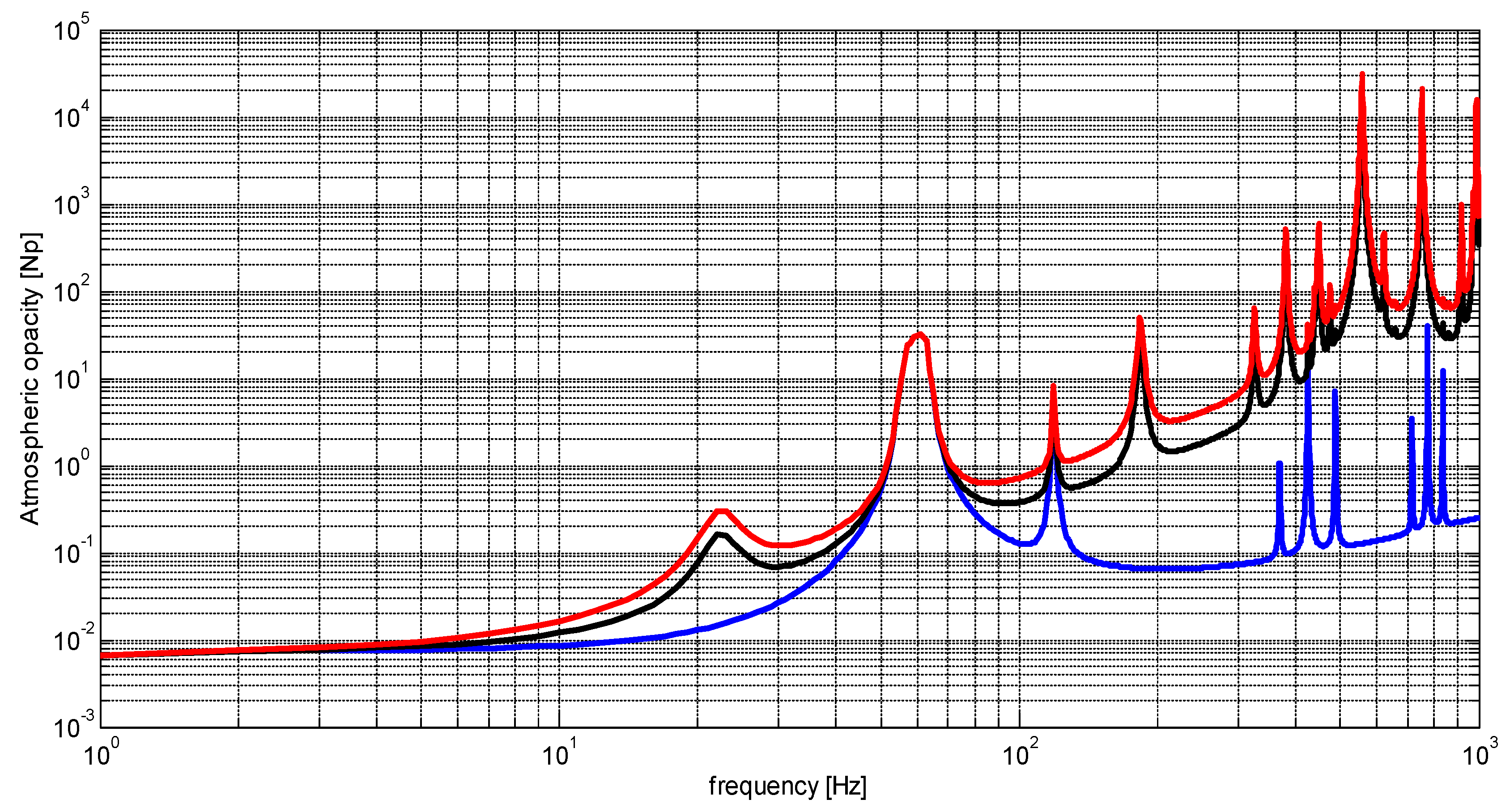
- Frequency range must cover at least from 1 to 100 GHz, to be able to address most land and ocean applications, e.g., 1.4 GHz (salinity, soil moisture), 6.9 GHz (sea surface temperature, sea wind speed), 10.65 GHz (wind speed), 18.7 GHz (sea wind speed, precipitation over sea, snow, ice), 23.8 GHz (total column water vapor), 31.4 GHz (precipitation over sea), 36.5 GHz (snow, ice), 54 GHz (precipitation over sea and land including height of the melting layer, temperature sounding), 89 GHz (thin snow, etc.). Frequencies above 100 GHz are only used for atmospheric applications, and fortunately in this case, most of the atmospheric models do perform well above this limit. The atmospheric attenuation models included are valid up to 1 THz.
- Introduction
- Materials and Methods
- 2.1. Main Building Blocks of a Synthetic Aperture Interferometric Radiometer Performance Simulator.
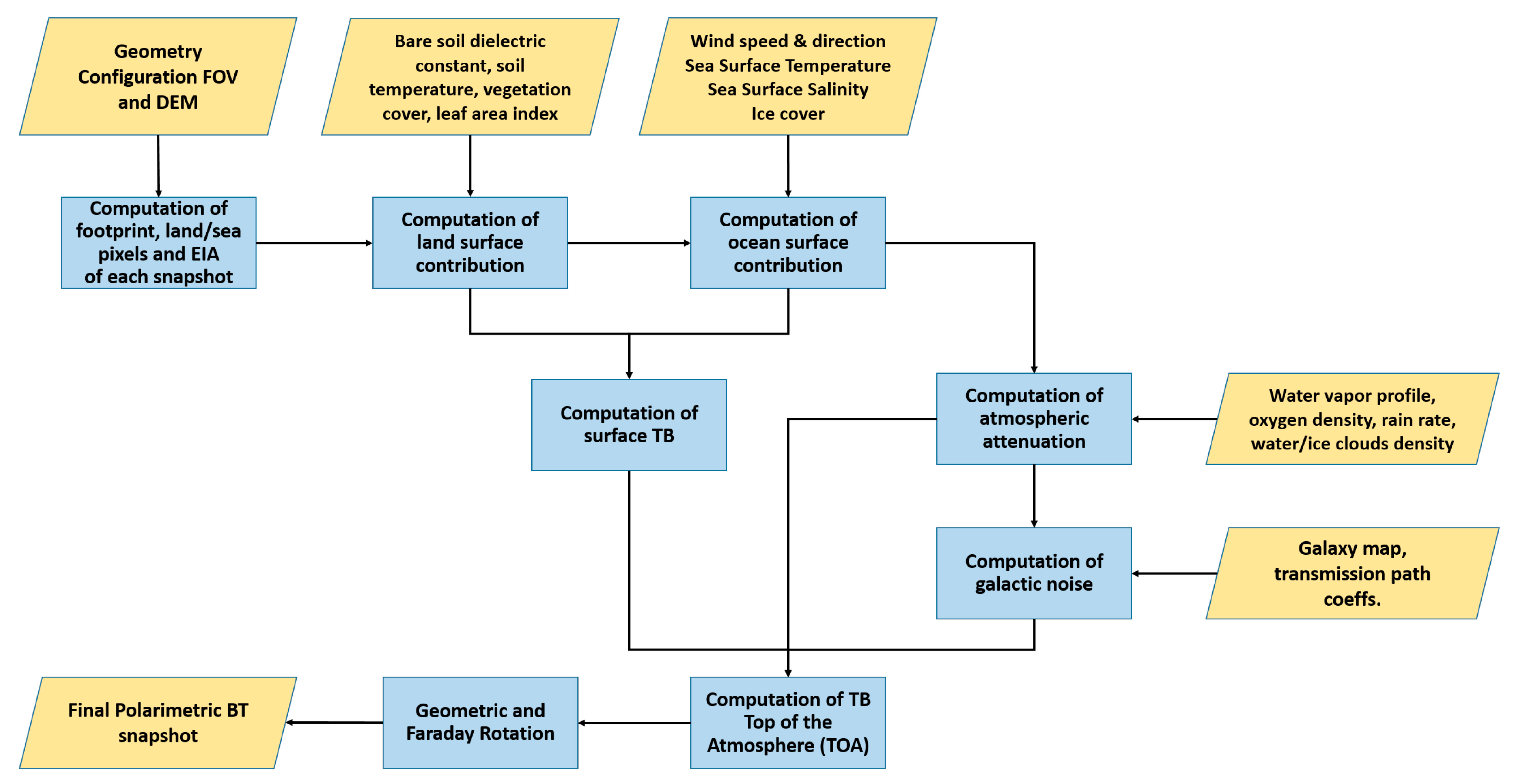
- 2.2. Radiative Transfer Module (RTM) block design
- 2.2.1. Earth’s surface contribution (dual-polarization)
- Land/Cryosphere Contributions
- A) Bare soil emission
- B) Vegetation-covered soils emission
- C) Ice and snow covered soils
- D) Other Effects including rocks, urban areas, inland water bodies, topography
- Ocean Surface Contributions (Fully Polarimetric)
- A) Flat Sea Surface Emissivity
- B) Isotropic Wind-induced Emissivity Signal
- C) Wind-directional Signal: Stokes Parameters
- D) Sea ice
- 2.2.2. Earth’s Atmosphere Contribution
- A) Water vapor attenuation
- B) Oxygen attenuation
- C) Rain attenuation
- D) Water clouds attenuation
- E) Ice clouds attenuation
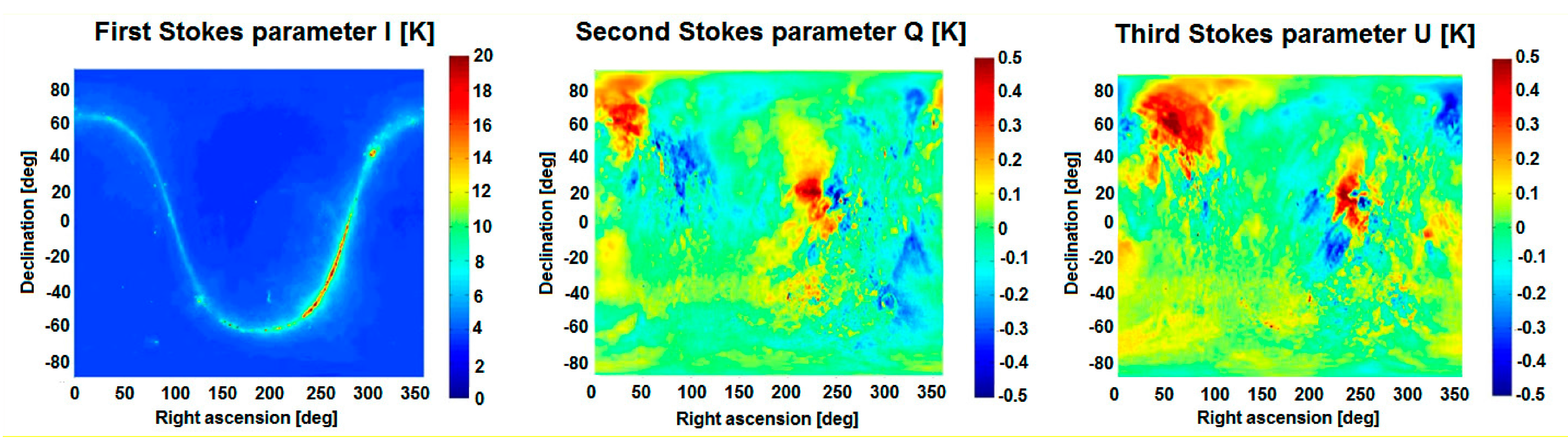
- 2.2.3. Cosmic, Isotropic, and Galactic Noises
- 2.2.4. Down-Welling Temperature Scattered Towards a Space-Borne Radiometer
- A) Over the land
- B) Over the ocean
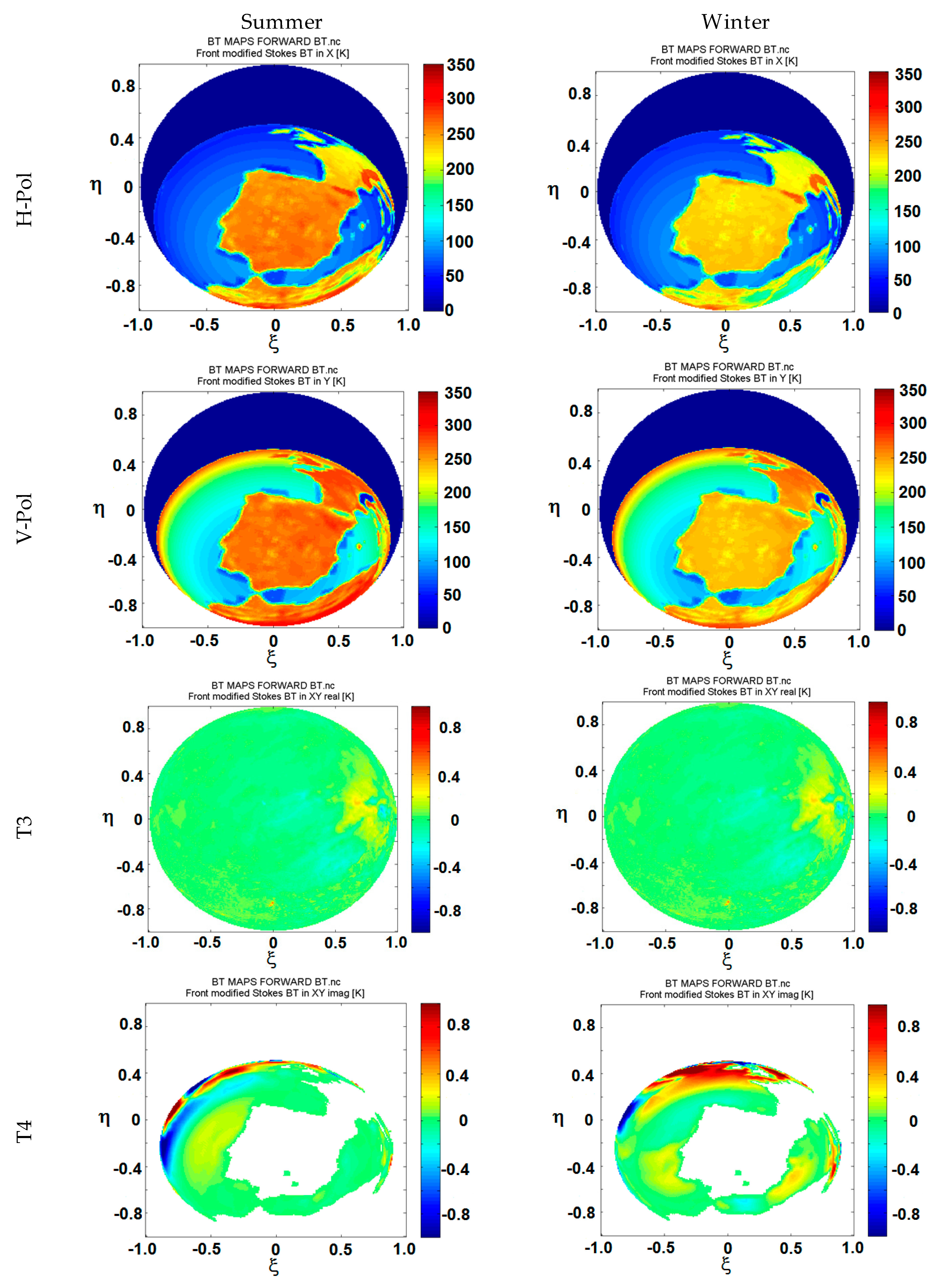
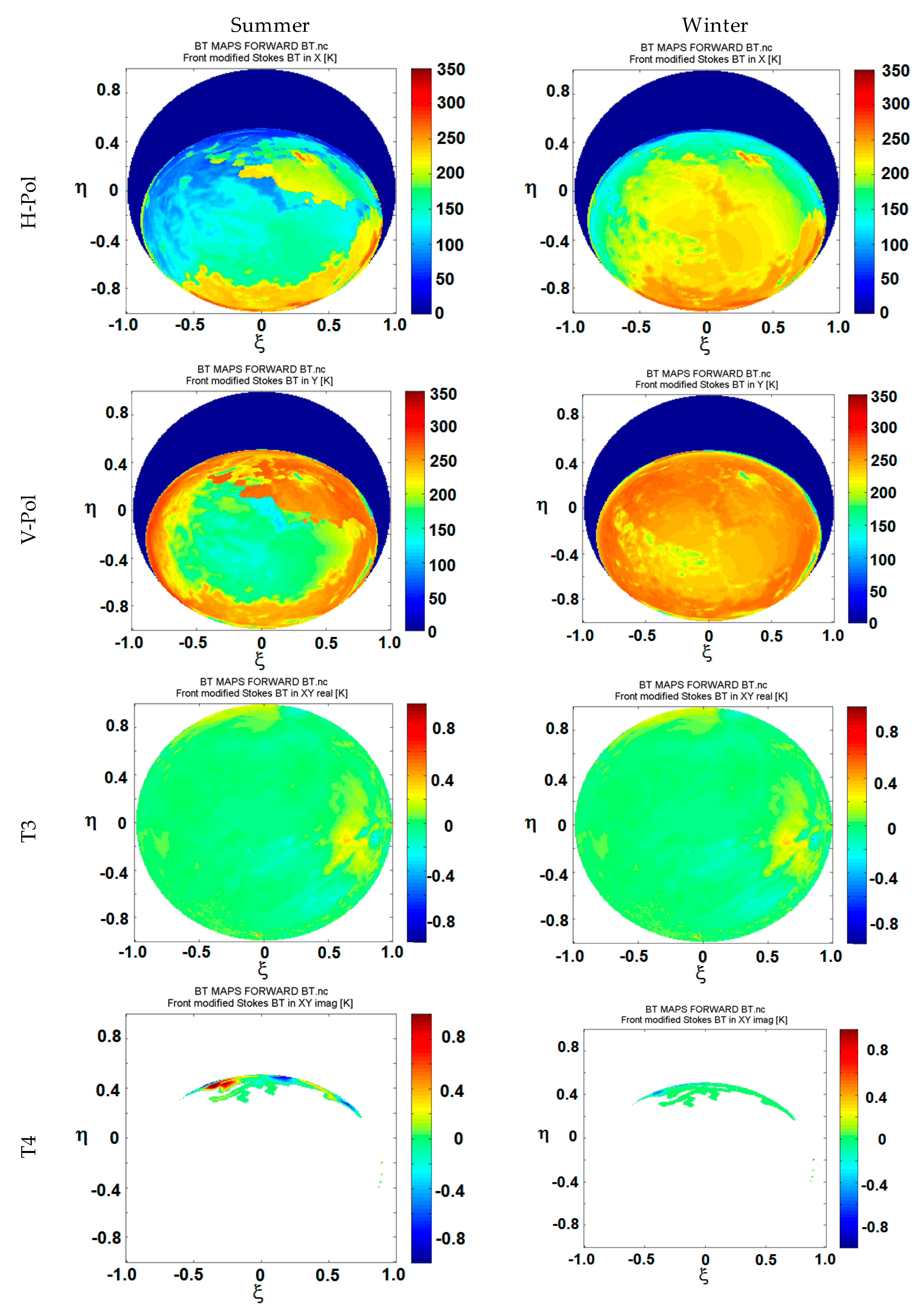
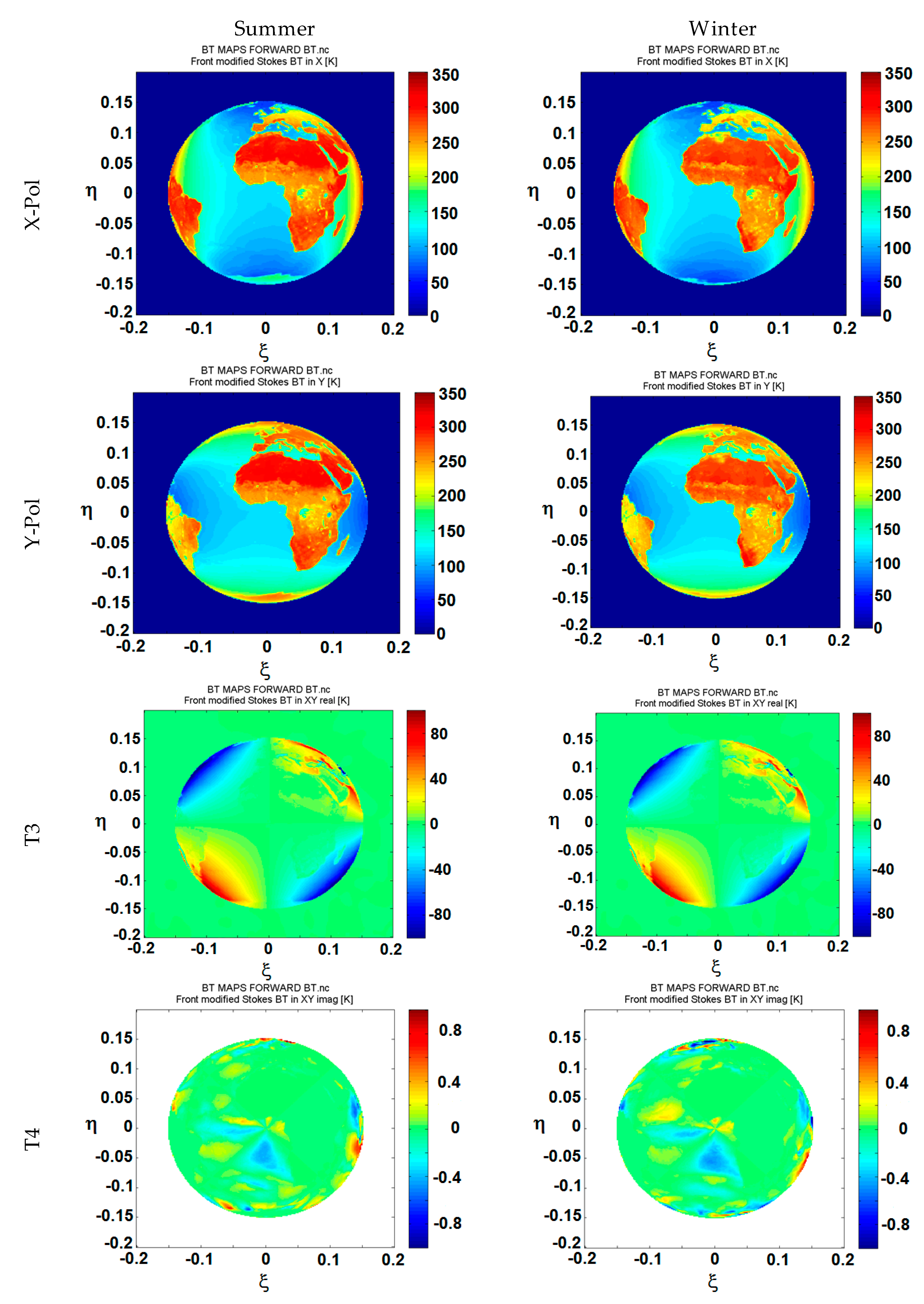
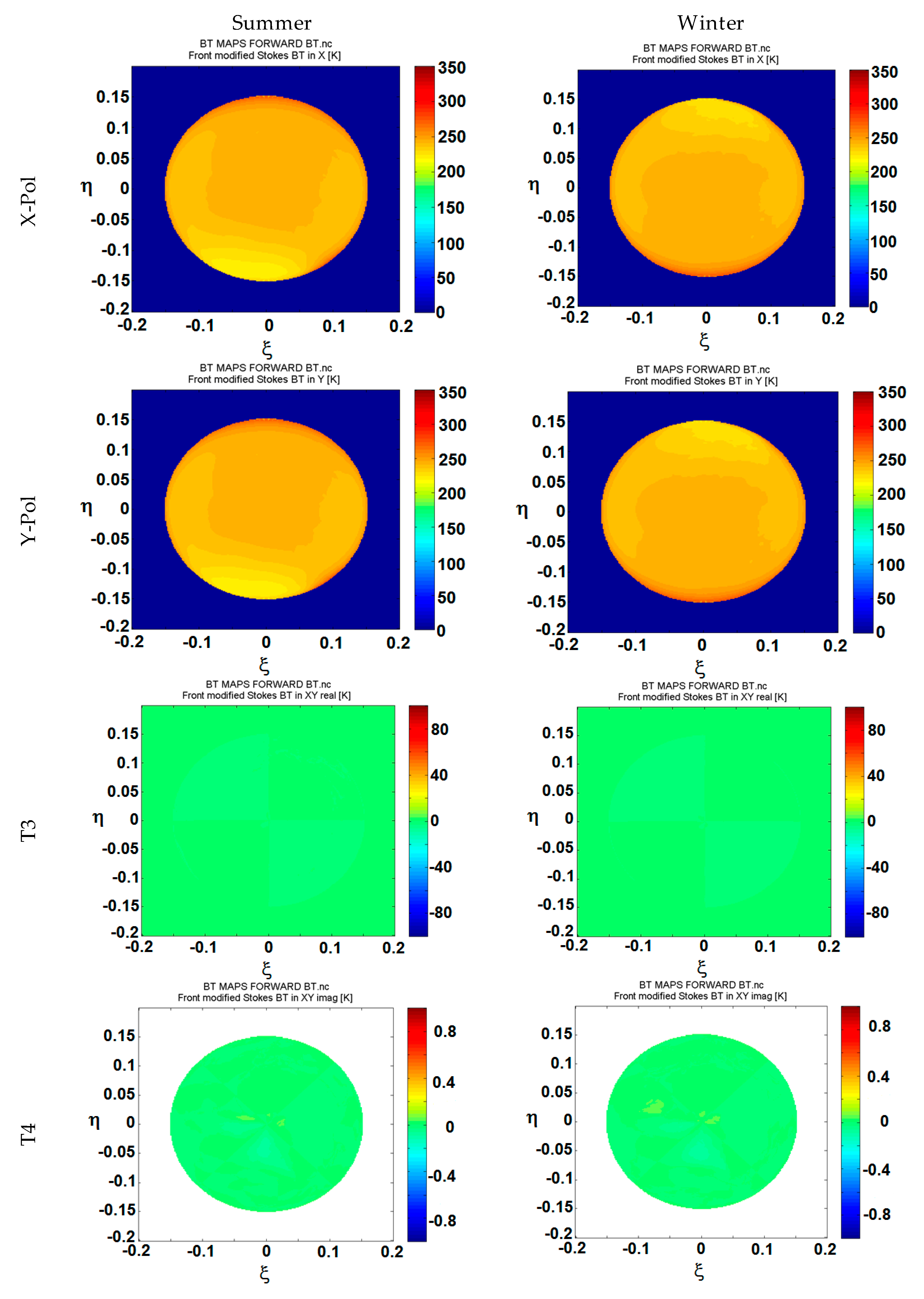
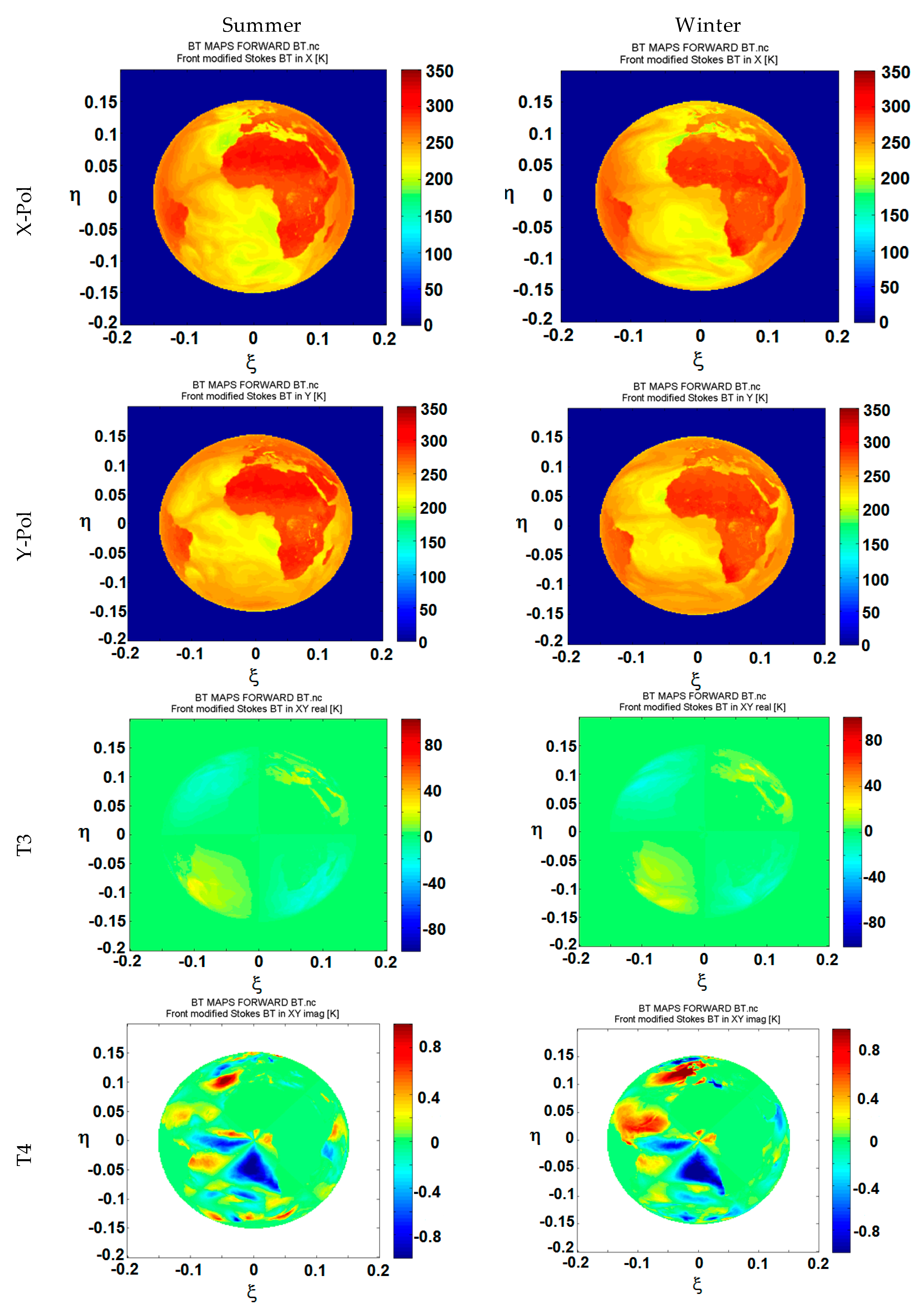
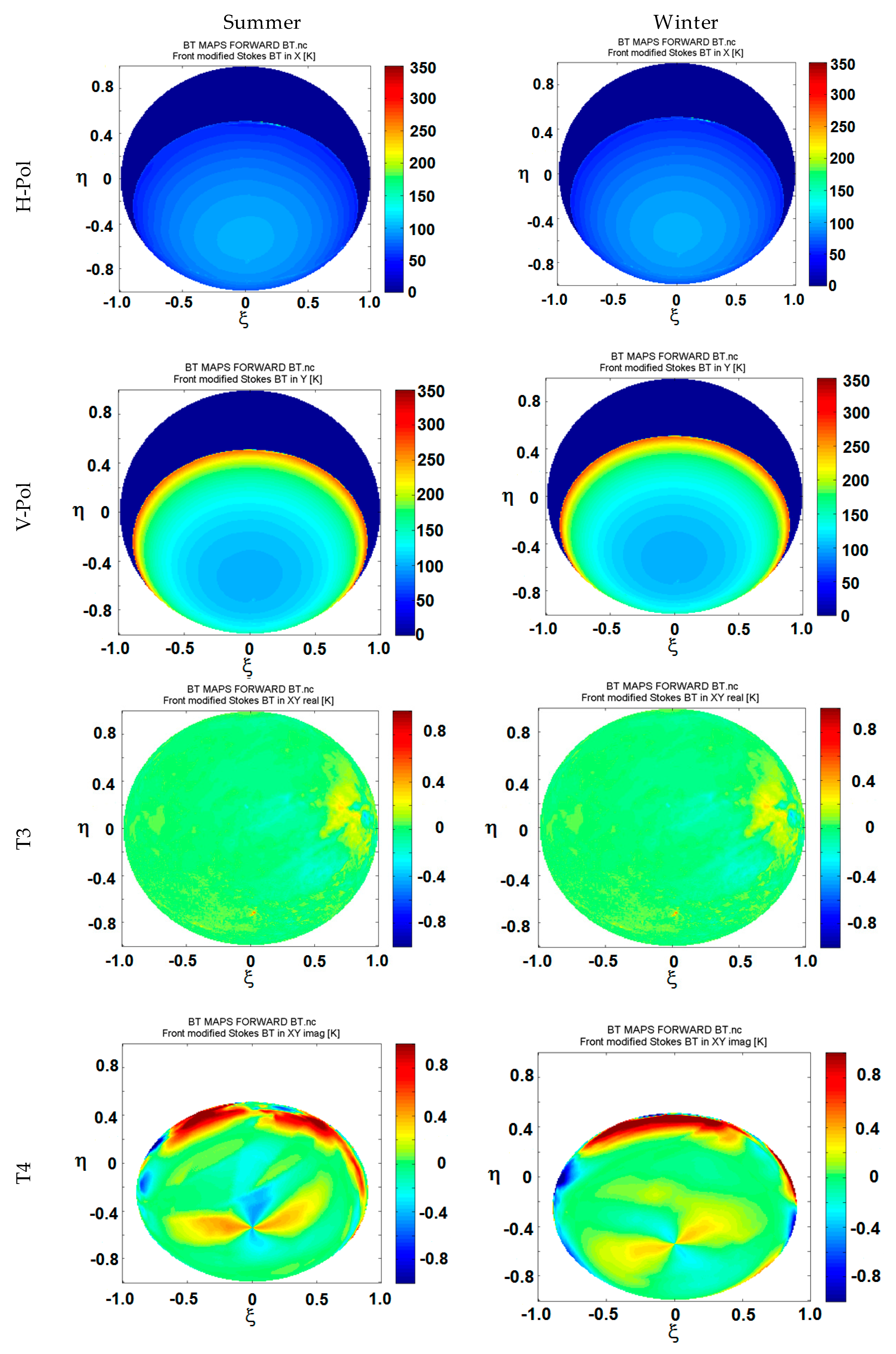
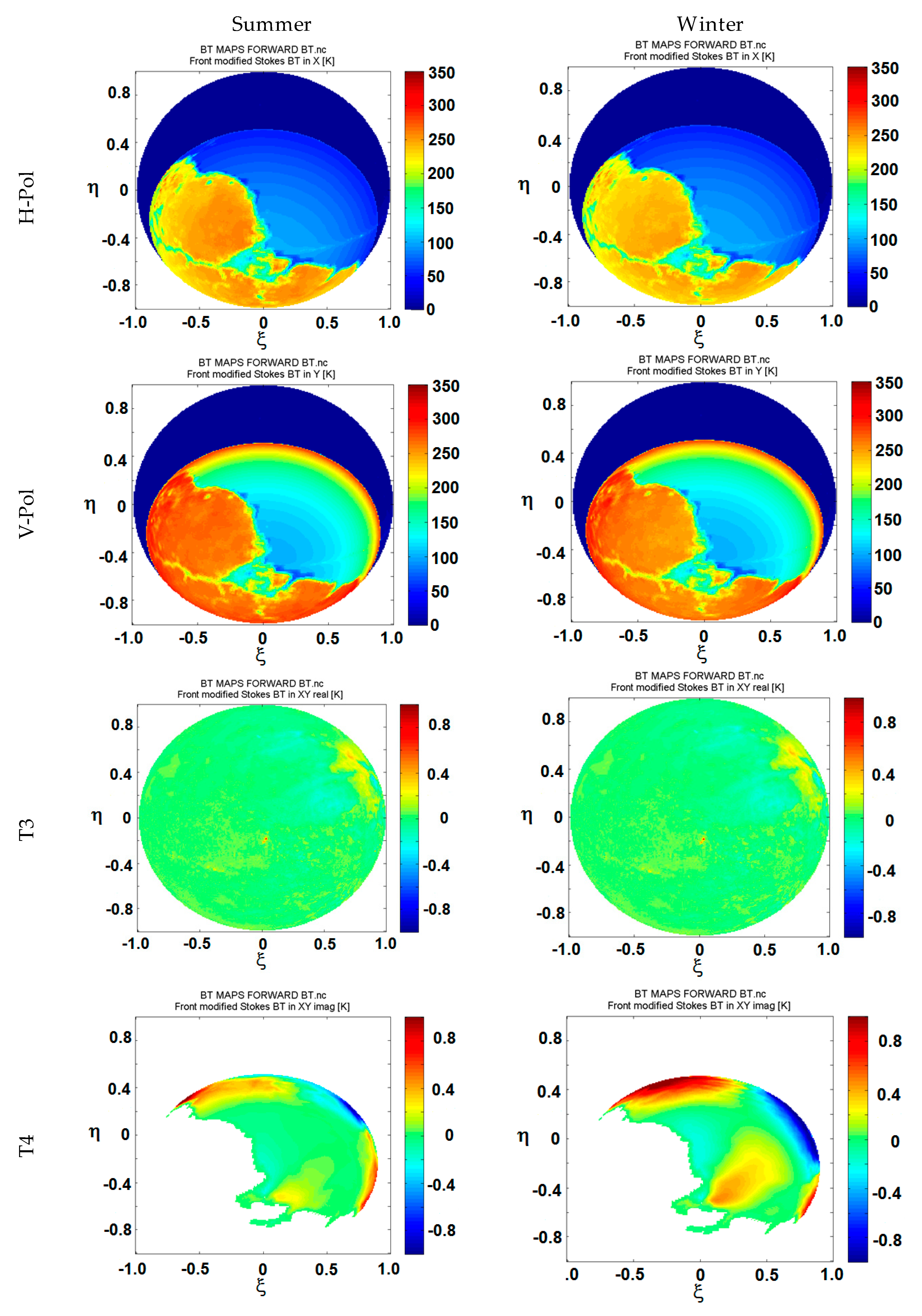
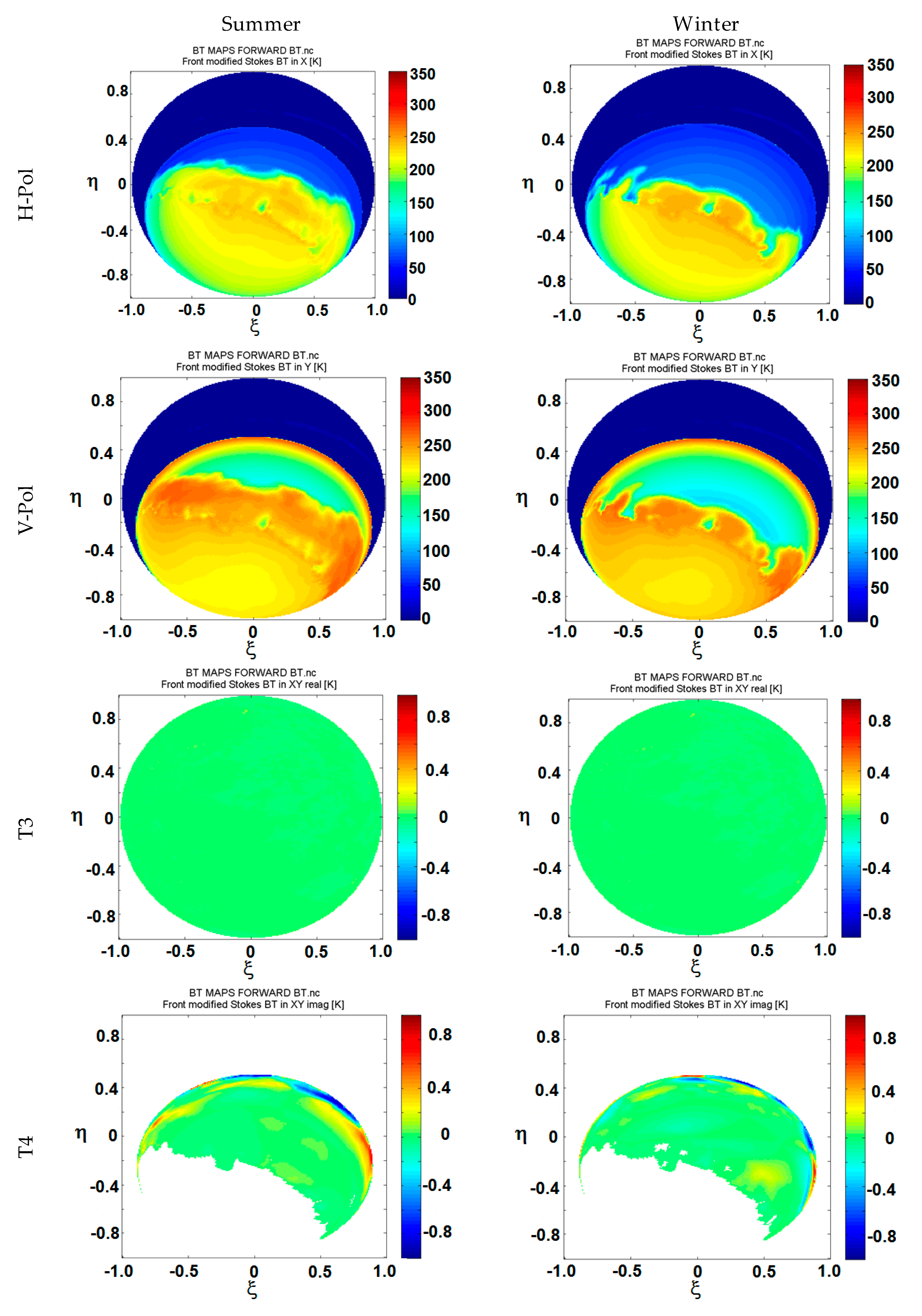
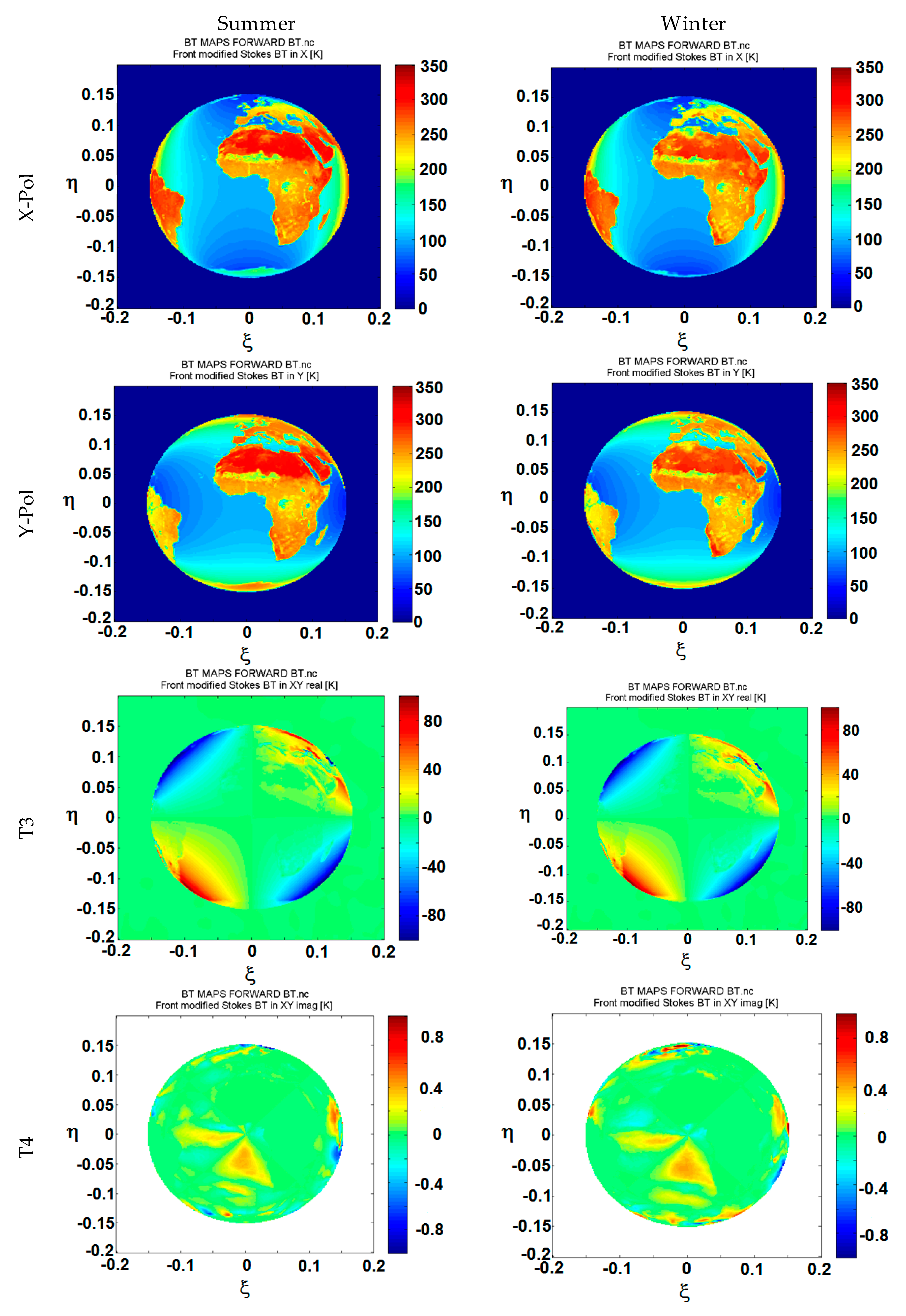
- 2.2.5. RTM Model Outputs
- 2.3. Input Data Collection and Strategy for Time- Space- Interpolation
- Simulation Results and Discussion
- Conclusions
2. Materials and Methods
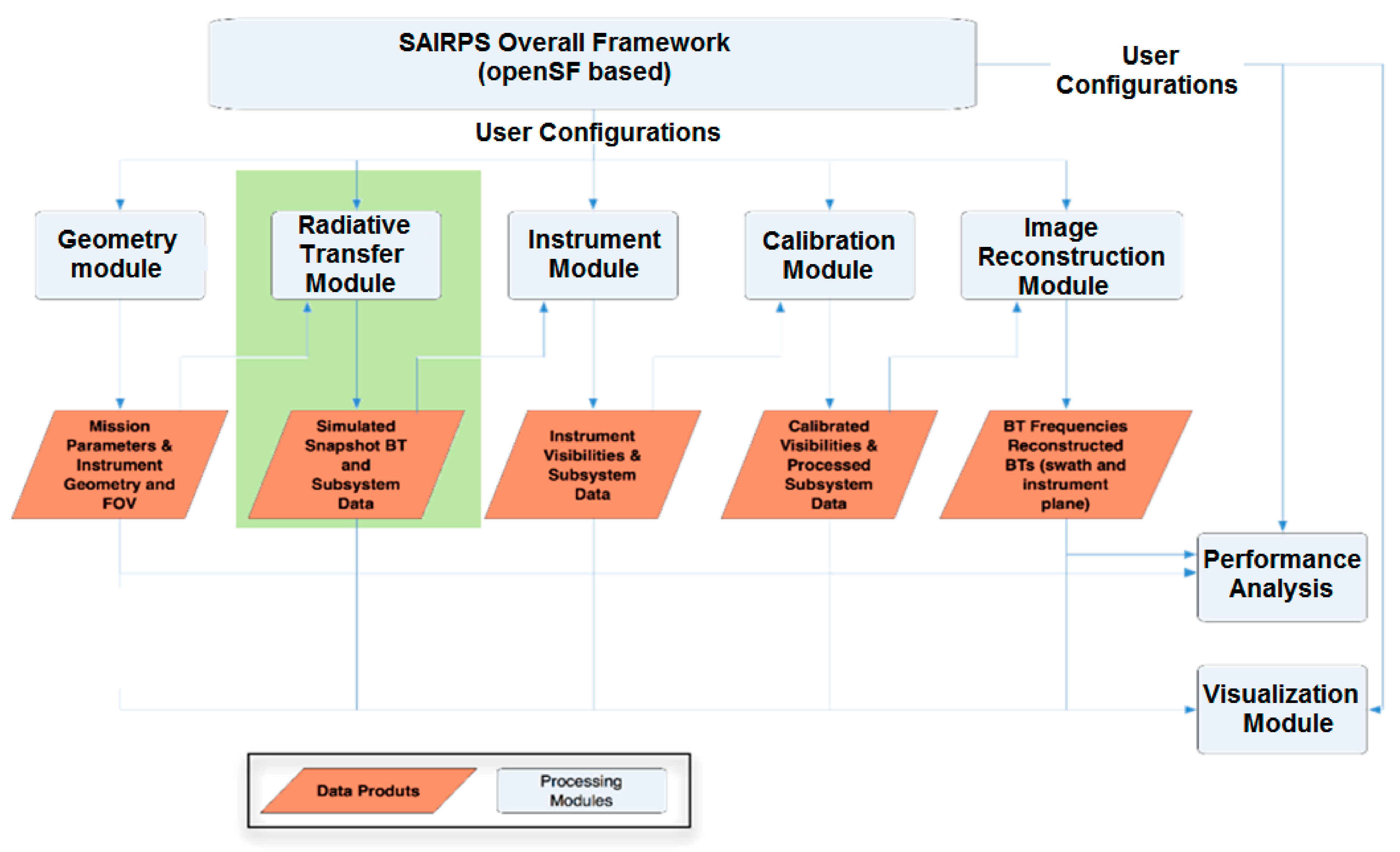
2.1. Main Building Blocks of a Synthetic Aperture Interferometric Radiometer Performance Simulator
- -
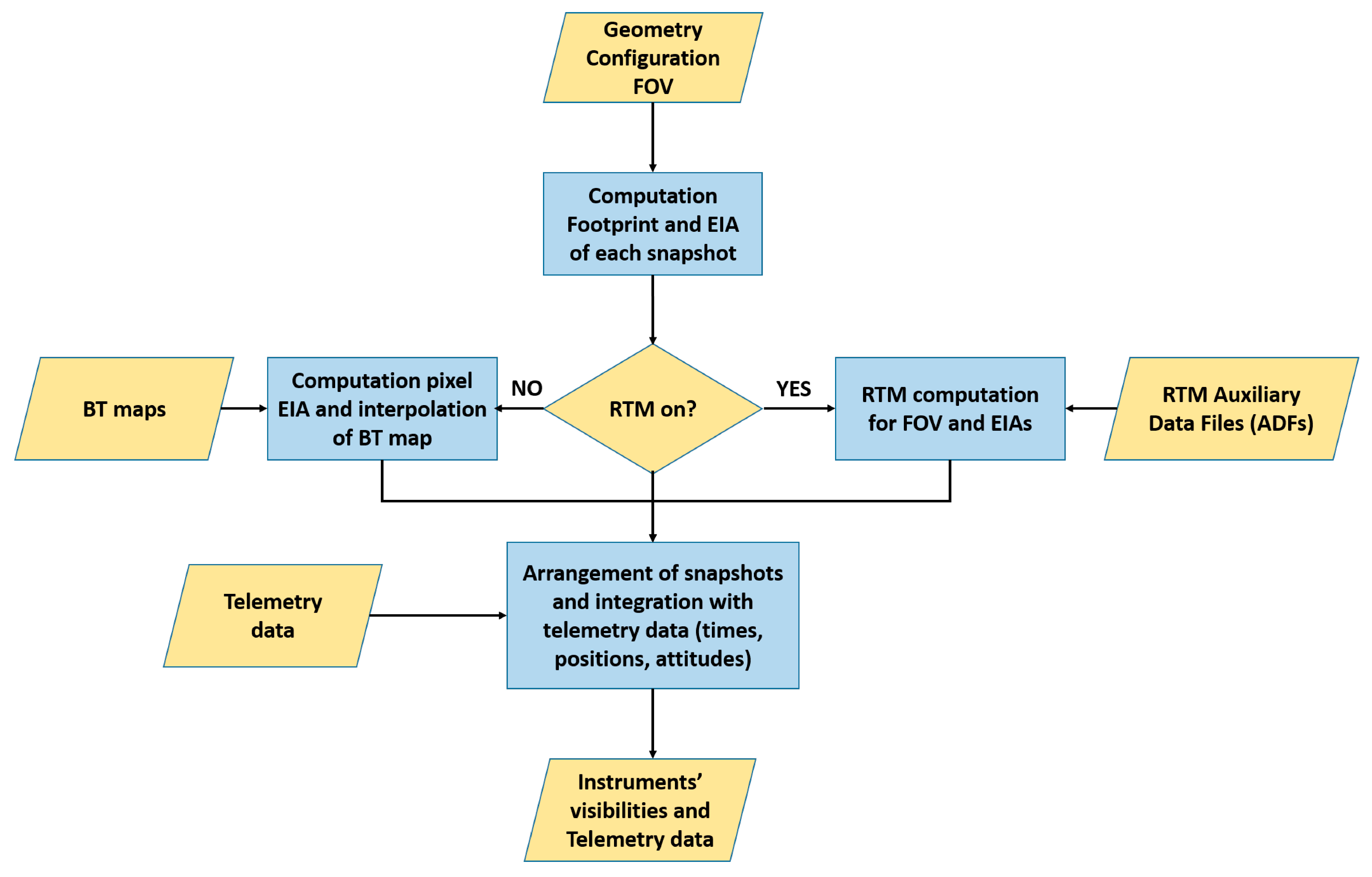
- The Geometry Module, which is capable of simulating arbitrary antenna positions and orientations (i.e., polarization or rotation) in the array, that are also defined individually as time-dependent variables (even within the integration time, which is subdivided in a number of subintervals to allow the simulation of image blurring, for example, due to instrument motion). The most common array configurations are provided as pre-defined standards and include: uniform linear array, Minimum (or Low) Redundancy Linear Array (MRLA or LRLA), star-like arrays with arbitrary number of arms, hexagonal arrays, circular arrays, U- and T-arrays… and the antenna spacing can be arbitrarily selected, or even be non-uniform in which case it will follow a geometric progression. It is also in this module that the orbital parameters are set, with a wide range of choices given to the user.
- -
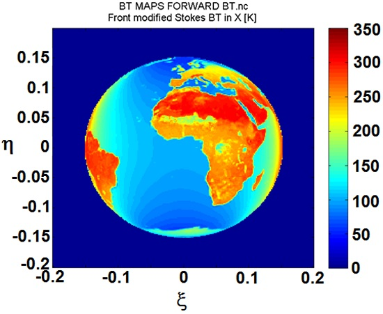
- The RTM and BT Maps Module that either computes the BT maps (4 Stokes parameters) at a given frequency and polarization, as a function of the incident and azimuth angles, and geophysical parameters, or ingests user defined BT maps, computing the FOV of the instrument and the surface area captured in each snapshot, according to the inputs given by the Geometry Module, and provide snapshot-based, interpolated, BT maps to the Instrument module. The RTM and BT maps module is detailed as shown in Figure 2, and it is the object of this manuscript.
- -
- The Instrument Module, which can simulate a generic receiver configuration. It includes the basic SAIR instrument components and their corresponding errors; the noise impact induced by instrument components; the physical temperature change impact; hardware non-idealities and uncertainties in the characterization of the instrument.
- -
- The Calibration Module is able to calculate the calibrated complex visibility samples from the raw observables produced by the Instrument Module. This module is able to simulate both internal and external calibrations.
- -
- The Image Reconstruction Module is able to produce a reconstructed brightness temperature map from the calibrated visibility samples, from the most basic image reconstruction method (a non-uniform FFT) [9], to the more sophisticated G-matrix method [10] (solved using either the Truncated Singular Value Decomposition, or the Conjugate Gradient), and the CLEAN method.Finally,
- -
- The Performance Module is used to evaluate the instrument’s performance in angular and radiometric resolutions.
- -
- Snapshot Mode to process a single BT snapshot, corresponding to the instrument elementary integration period, in order to compare against the reference BT maps,
- -
- Monte-Carlo Mode to evaluate the instrument performance by analyzing a sequence of consecutive snapshots for a given constant brightness temperature map. A set of system/instrument random errors can be included in the simulation and the user has the possibility to select which of the components parameters are fixed and which ones are allowed to vary according to its configuration.
- -
- Time Evolution Mode to analyze instrument’s drifts or to generate synthetic multi-look observations to simulate the actual instrument performance and develop geophysical parameters retrieval algorithms.
2.2. RTM block Design
- -
- Land surface contribution computation, including bare soil emission, vegetation-covered soils emission, ice and snow, and other effects, such as rocky soil, urban areas, inland water bodies, and topography effects,
- -
- Ocean surface contribution computation, including flat sea emission, and wind effects and the induced azimuthal signature in the four Stokes parameters,
- -
- Atmosphere attenuation computation (scattering effects are not included), and
- -
- Sky contribution computation, including direct and reflection contributions over land and over sea.
2.2.1. Earth’s Surface Contribution
Land/Cryosphere Contributions
A. Bare Soil Emission
- Flat soil emission: for smooth bare soils, the reflection coefficients are given by the (power) Fresnel reflection coefficients as given by:where εr is the dielectric constant and the soil is assumed to be a non-magnetic medium (μr = 1).
- Surface’s roughness effects are accounted for by using a “rough” surface reflectivity that is computed using the following empirical relationship:where Q is the so-called polarization mixing factor , HR is an effective surface’s roughness (no units), and NRp is a polarization-dependent integer between 0 and 2 used to parameterize the roughness effects of the incidence angle [19].
- The effective soil temperature (Ts) depends on the soil properties and moisture content profile within the soil volume. The effective temperature is usually computed using a surface temperature and the temperature at a depth where it is almost constant. The actual profile and depth are dependent upon the soil type actual profile and the level at which the deep soil temperature is obtained. The effective soil temperature is written as a function of the soil temperature at depth (Tsoil depth, approximately at 0.5 m depth), and surface soil temperature (Tsoil surf, approximately at 5 cm) as follows:where:is a parameter depending mainly on the frequency and the soil moisture. If the soil is very dry, soil layers at depth (deeper than one meter for dry sand) contribute significantly to the soil emission, and the value of Ct is lower than 0.5. Conversely, if the soil is very wet, the soil emission originates mainly from layers at the soil surface and Ct ≈ 1. In Equation (19) w0 and bw0 are parameters that depend mainly on the soil texture and structure. Often it can be assumed that .
B. Vegetation-Covered Soils Emission
- For low vegetation, the τ-ω model is given by:where the first term corresponds to the soil emission attenuated by the vegetation canopy, the second one corresponds to the vegetation upwelling emission including the first order scattering through the single scattering albedo (), and the third one to the vegetation down-welling emission reflected on the soil surface, and then attenuated and scattered in the vegetation in the upwelling path. The vegetation layer attenuation is , where is the nadir optical depth of the vegetation layer.
- Over forests, a simple τ-ω empirical approach is not entirely appropriate because the emission/scattering processes are more complex. Since trunks and branches are comparable in size to the electromagnetic wavelength, multiple scattering effects cannot be neglected, and a simple first-order approach is not reliable [23,24,25]. Despite the above considerations, from an operational point of view, a simple τ-ω approach is kept here, as it is in the SMOS L2 Soil Moisture processor. Three forest categories are aggregated: (1) needle leaf and broadleaf (including Tropical forests and woodland); (2) mixed forests; and (3) woodlands. The same general procedure is applied for the 3 categories as in the low vegetation case, although the parameters are specific of each category:where FV is the fraction of the LAI corresponding to the understory contribution.
C) Ice and Snow Covered Soils
- Frozen soils cover large areas at high latitudes and sometimes altitudes. At mid latitudes, frozen soil can also be expected in winter, especially for morning-pass orbits (e.g., 6 AM). Experience shows that the dielectric properties of frozen soil are very close to those of dry soil, while vegetation is almost fully transparent [26]. It is often considered that for frozen soils the dielectric constant can be written [27].
- Ice covered soils emission is computed in a similar way [28], but the dielectric constant of the ice layer should be used instead. The input parameters are the temperature (T in [K]) and the frequency (f in [GHz]):
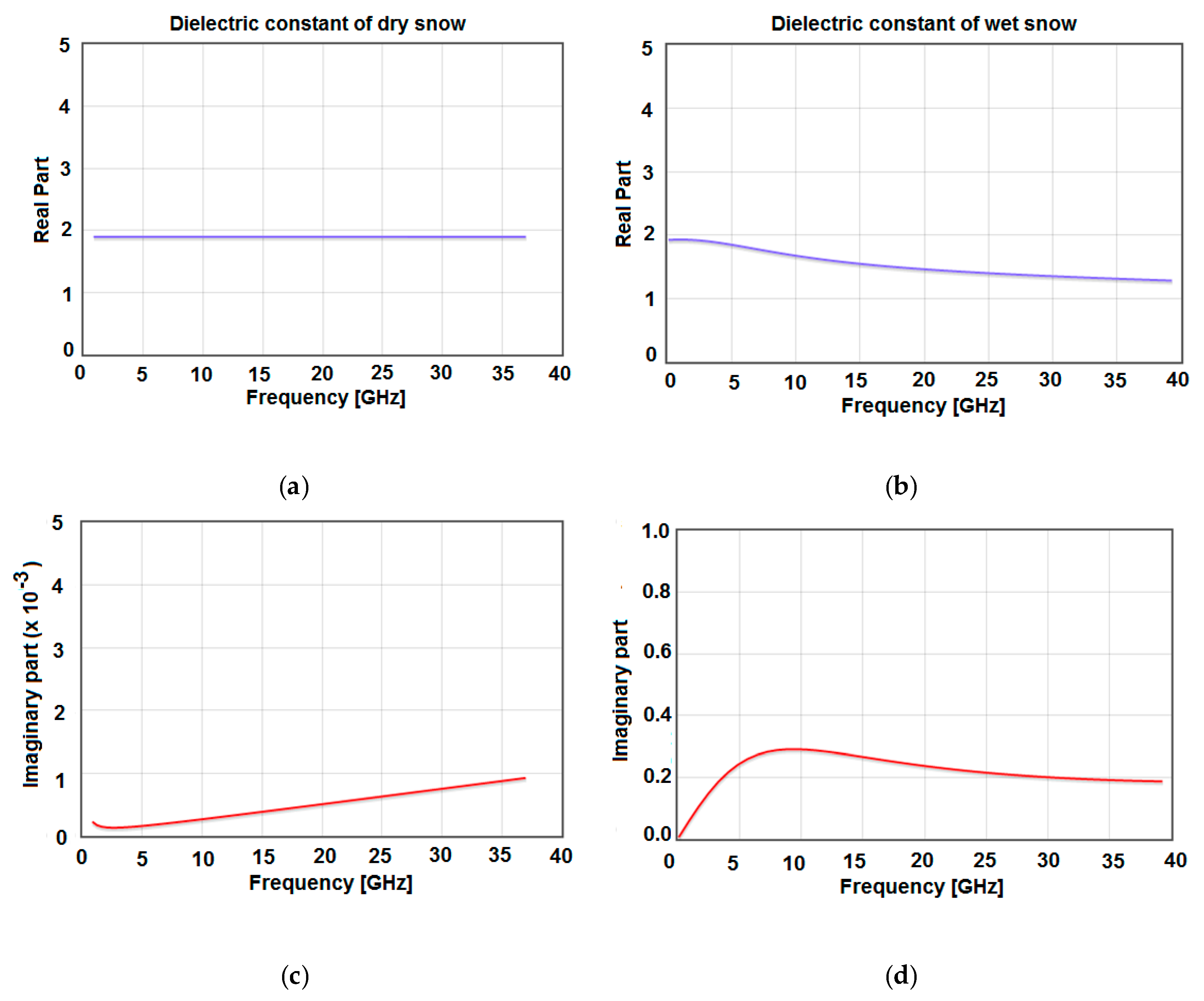
- Snow covered soils account for about 40% of the Northern hemisphere land mass, and it varies seasonally. Dielectric properties depend on its history: while fresh, dry snow is transparent to microwave radiation; as snow melts its dielectric constant increases, snow grain size and liquid water content increase and may be totally opaque (at 0 °C) when wet.
D) Other Effects
- Rocks and rocky outcrops areas are not well modelled at present. They are assumed to behave as very dry soils. Field measurements do not show a significant effect from rocks, which are usually encountered in barren areas or in mountains regions, etc. In [20] permittivity values are given for rocks at 400 MHz and 35 GHz. They range from 2.4 to 9.6. Approximate expressions do exist for rocks, but a default constant dielectric constant value is usually assumed:
- Urban Areas are usually largely covered by concrete and asphalt, therefore a bare soil model is used, but using the dielectric constant of dry asphalt.
- Inland Water Bodies and Rivers are modelled using a “flat” “bare soil model” with (Q = 0) and using the fresh water dielectric constant model, which depends on the frequency and temperature (salinity is assumed to be equal to zero). In [29] a model is presented that has been validated from 19 to 86 GHz data, and in its derivation it included data up to 500 GHz. The implementation used in this project follows that of [28], which is applicable for frequencies (f) up to 1 THz, physical temperature (T) from 0 °C to 30 °C, and salinities (S) from 0 to 40 psu. Please note that the formulas below will be used in the sea surface emissivity calculation with the appropriate value of salinity S (≠0).
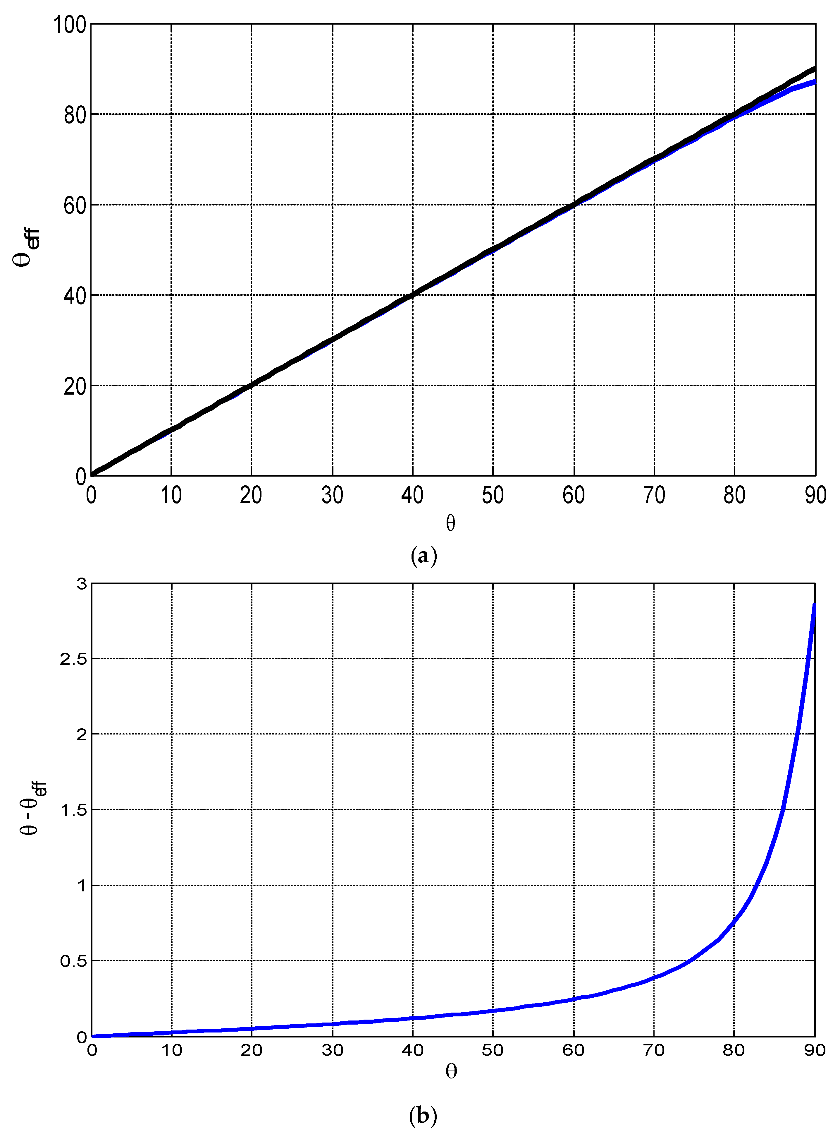
- Topography effects produce a change of the local incidence angle, polarization mixing, and eventually a shadowing and multiple scattering, which are not accounted for in this model. The equations to compute the scattered field components from the illuminating wave components are summarized below [30]:where the effective (electric field amplitude) reflection coefficients are given by:and and are the Fresnel reflection coefficients for the electric field (or the modified ones to account for surface roughness, vegetation, etc.) at v and h polarizations. The power reflection coefficients were derived by taking the square of the module of the (amplitude) electric field reflection coefficients. The angle between the facet and the observation direction is given by:where is the normal to the facet, which exhibits a tilt angle α, oriented by an azimuth angle β with respect to the global plane of incidence. The other unitary vectors are defined as follows:
Ocean Surface Contributions
A) Flat Sea Surface Emissivity
B) Isotropic Wind-induced Emissivity Signal
C) Wind-directional Signal: Stokes Parameters
D) Sea ice
2.2.2. Earth’s Atmosphere Contribution
A) Water Vapor Attenuation
B) Oxygen Attenuation
C) Rain Attenuation
D) Water Clouds Attenuation
E) Ice Clouds Attenuation
2.2.3. Cosmic, Isotropic, and Galactic Noises
- The cosmic background is fairly constant and equal to .
- The isotropic component (extra-galactic term) decreases with frequency roughly as:
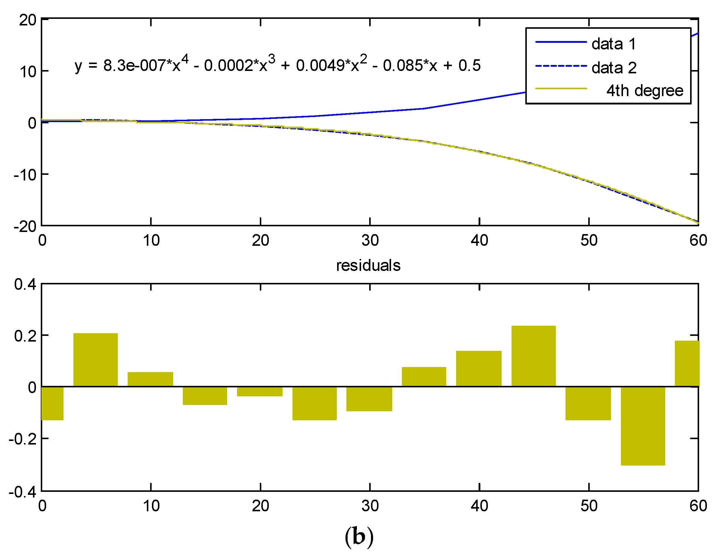
- The galactic component also decreases with frequency roughly as:where β lies between 2.5 and 2.6 between 45 and 408 MHz, and it is equal to 2.81 ± 0.16 from 1.375 to 7.5 GHz. A Global Sky Model derived from all publicly available unpolarized large-area radio surveys can be found at [42]. In the framework of this simulation tool the map used in the SMOS processors, scaled according to Equation (118) with β = 2.81, is used (Figure 9).
2.2.4. Down-Welling Temperature Scattered Towards a Space-Borne Radiometer
A) Over the Land
B) Over the Ocean
2.2.5. RTM Model Outputs
2.3. Input Data Collection and Strategy for Time- Space- Interpolation
- grid point identifier, latitude, longitude, surface height over the ellipsoid [m], land-sea mask (using a 0.5 threshold),
- sea-ice cover [%], sea surface temperature [K], ice surface temperature [K], 10 m height wind speed [m/s], 10 m height neutral equivalent wind speed – zonal and meridional components [m/s], and sea surface salinity [psu],
- volumetric soil water content [m3/ m3], soil surface temperature [K], temperature of the snow layer [K], ice surface temperature [K], snow depth [m], snow water equivalent [m], snow density [kg/m], fractions [%] of vegetated soil, forest, wetlands, open fresh water, open saline water, barren, ice and permanent snow, urban area, strong and moderate topography, leaf area index (LAI) [m2/m2], vegetation opacity at nadir [Np] for low vegetation and forests, surface roughness parameter [-], soil percentage of sand and clay [%], soil bulk density [g/cm3], w0 [m3/m3] and bw0 [-] parameters for the computation of the effective soil temperature, XMVT [-] transition moisture point and field capacity [-] as a function of the sand and clay fractions, surface soil moisture [m3/m3],
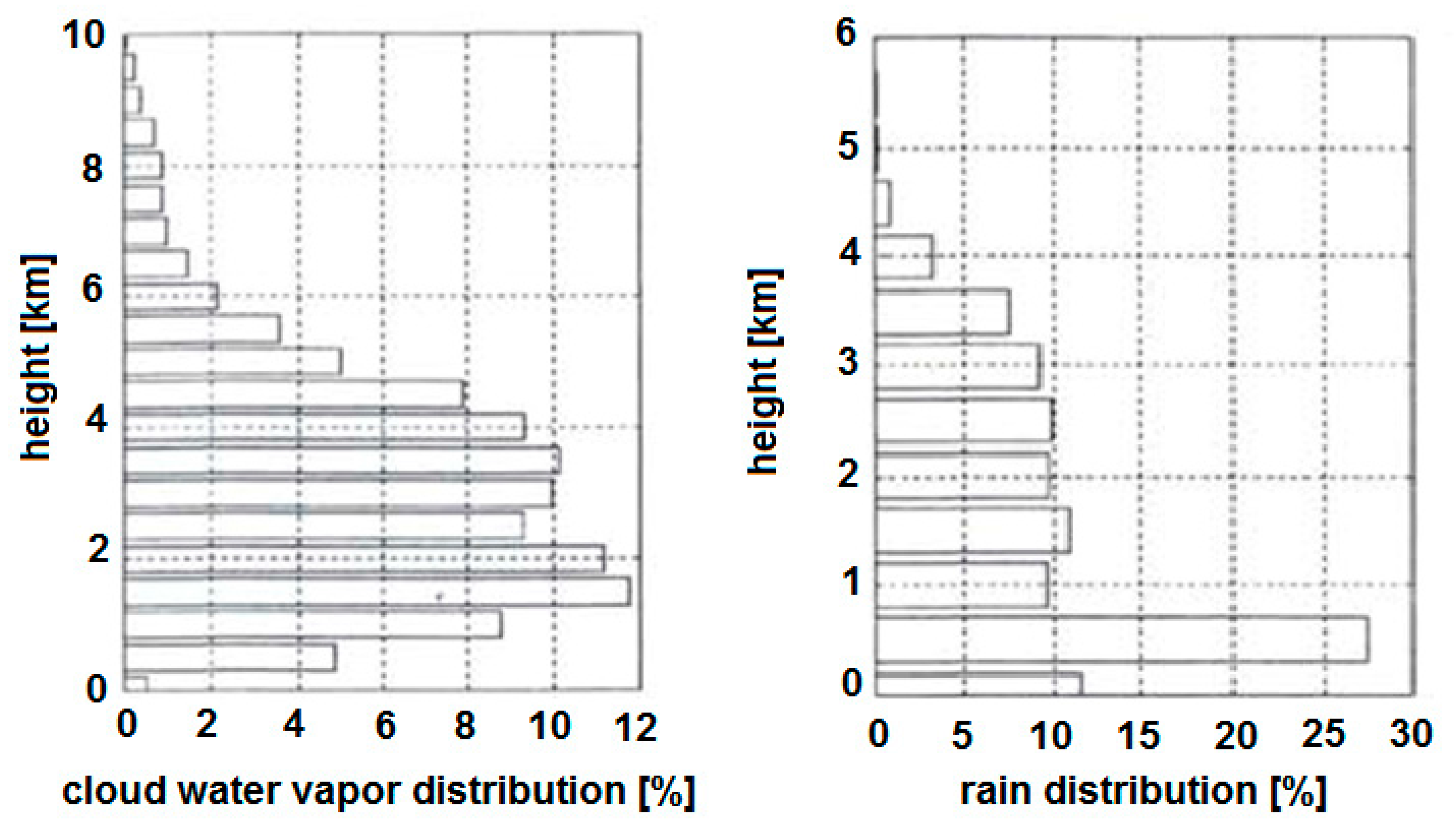
- temperature [K] and relative humidity [%] as a function of the atmospheric pressure [Pa], specific cloud liquid water content [kg/kg], specific cloud ice water content [kg/kg], specific rain water content [kg/kg], and specific snow water content [kg/kg].
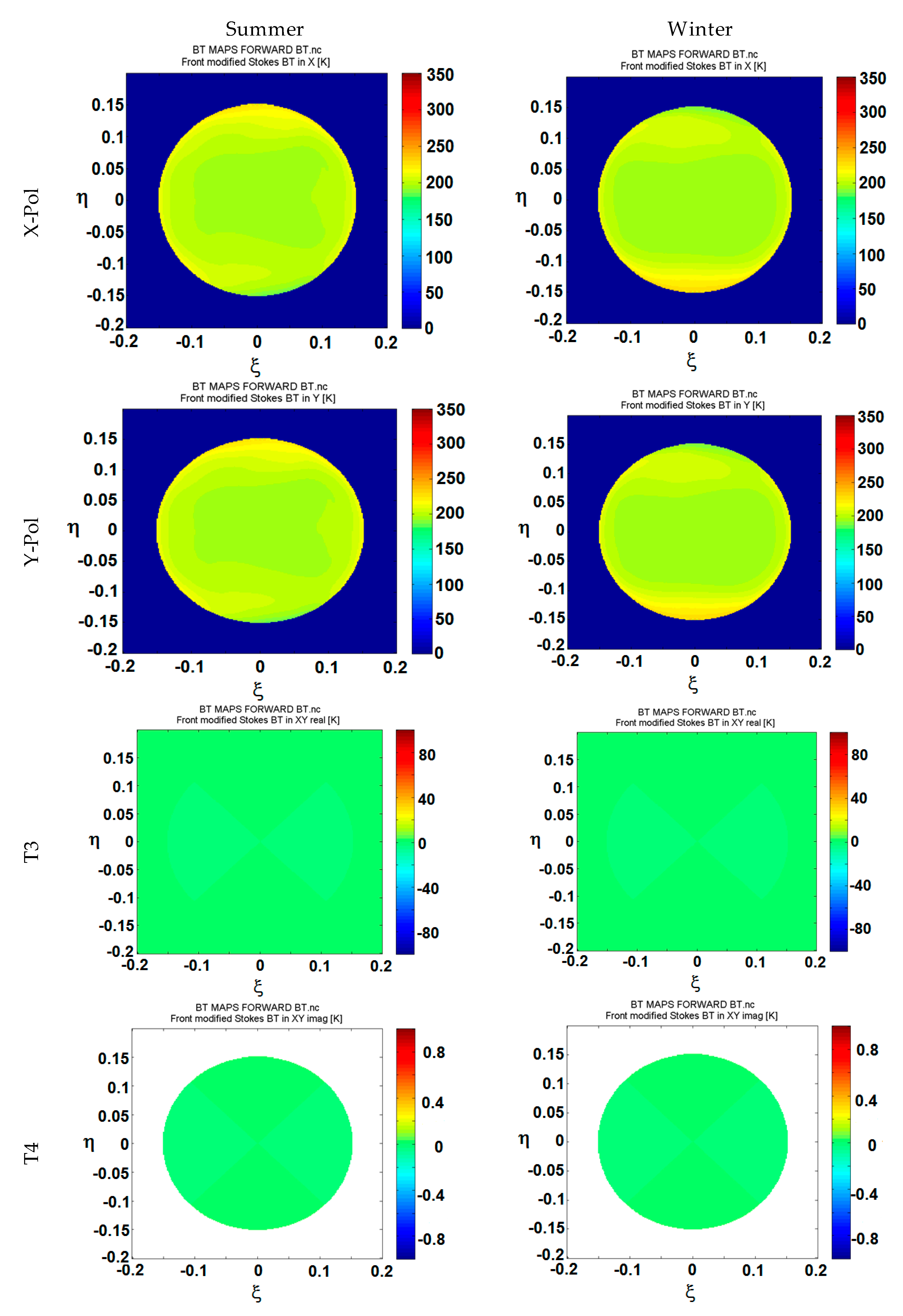
3. Simulation Results and Discussion
4. Conclusions
Acknowledgments
Author Contributions
Conflicts of Interest
Appendix

| νi [GHz] | ai | bi | ci | di | ei | fi |
|---|---|---|---|---|---|---|
| 22,235080 | 0,01130 | 2,143 | 2,811 | 4,80 | 0,69 | 1,00 |
| 67,803960 | 0,00012 | 8,735 | 2,858 | 4,93 | 0,69 | 0,82 |
| 119,995940 | 0,00008 | 8,356 | 2,948 | 4,78 | 0,70 | 0,79 |
| 183,310091 | 0,24200 | 0,668 | 3,050 | 5,30 | 0,64 | 0,85 |
| 321,225644 | 0,00483 | 6,181 | 2,303 | 4,69 | 0,67 | 0,54 |
| 325,152919 | 0,14990 | 1,540 | 2,783 | 4,85 | 0,68 | 0,74 |
| 336,222601 | 0,00011 | 9,829 | 2,693 | 4,74 | 0,69 | 0,61 |
| 380,197372 | 1,15200 | 1,048 | 2,873 | 5,38 | 0,54 | 0,89 |
| 390,134508 | 0,00046 | 7,350 | 2,152 | 4,81 | 0,63 | 0,55 |
| 437,346667 | 0,00650 | 5,050 | 1,845 | 4,23 | 0,60 | 0,48 |
| 439,150812 | 0,09218 | 3,596 | 2,100 | 4,29 | 0,63 | 0,52 |
| 443,018295 | 0,01976 | 5,050 | 1,860 | 4,23 | 0,60 | 0,50 |
| 448,001075 | 1,03200 | 1,405 | 2,632 | 4,84 | 0,66 | 0,67 |
| 470,888947 | 0,03297 | 3,599 | 2,152 | 4,57 | 0,66 | 0,65 |
| 474,689127 | 0,12620 | 2,381 | 2,355 | 4,65 | 0,65 | 0,64 |
| 488,491133 | 0,02520 | 2,853 | 2,602 | 5,04 | 0,69 | 0,72 |
| 503,568532 | 0,00390 | 6,733 | 1,612 | 3,98 | 0,61 | 0,43 |
| 504,482692 | 0,00130 | 6,733 | 1,612 | 4,01 | 0,61 | 0,45 |
| 547,676440 | 0,97010 | 0,114 | 2,600 | 4,50 | 0,70 | 1,00 |
| 552,020960 | 1,47700 | 0,114 | 2,600 | 4,50 | 0,70 | 1,00 |
| 556,936002 | 48,74000 | 0,159 | 3,210 | 4,11 | 0,69 | 1,00 |
| 620,700807 | 0,50120 | 2,200 | 2,438 | 4,68 | 0,71 | 0,68 |
| 645,866155 | 0,00713 | 8,580 | 1,800 | 4,00 | 0,60 | 0,50 |
| 658,005280 | 0,03022 | 7,820 | 3,210 | 4,14 | 0,69 | 1,00 |
| 752,033227 | 23,96000 | 0,396 | 3,060 | 4,09 | 0,68 | 0,84 |
| 841,053973 | 0,00140 | 8,180 | 1,590 | 5,76 | 0,33 | 0,45 |
| 859,962313 | 0,01472 | 7,989 | 3,060 | 4,09 | 0,68 | 0,84 |
| 899,306675 | 0,00605 | 7,917 | 2,985 | 4,53 | 0,68 | 0,90 |
| 902,616173 | 0,00426 | 8,432 | 2,865 | 5,10 | 0,70 | 0,95 |
| 906,207325 | 0,01876 | 5,111 | 2,408 | 4,70 | 0,70 | 0,53 |
| 916,171582 | 0,83400 | 1,442 | 2,670 | 4,78 | 0,70 | 0,78 |
| 923,118427 | 0,00869 | 10,220 | 2,900 | 5,00 | 0,70 | 0,80 |
| 970,315022 | 0,89720 | 1,920 | 2,550 | 4,94 | 0,64 | 0,67 |
| 987,926764 | 13,21000 | 0,258 | 2,985 | 4,55 | 0,68 | 0,90 |
| νi [GHz] | ai (x 10−6) | bi | ci | di | ei | fi |
|---|---|---|---|---|---|---|
| 50,474238 | 0,094 | 9,694 | 0,89 | 0,80 | 0,240 | 0,790 |
| 50,987749 | 0,246 | 8,694 | 0,91 | 0,80 | 0,220 | 0,780 |
| 51,503350 | 0,608 | 7,744 | 0,94 | 0,80 | 0,197 | 0,774 |
| 52,021410 | 1,414 | 6,844 | 0,97 | 0,80 | 0,166 | 0,764 |
| 52,542394 | 3,102 | 6,004 | 0,99 | 0,80 | 0,136 | 0,751 |
| 53,066907 | 6,410 | 5,224 | 1,02 | 0,80 | 0,131 | 0,714 |
| 53,595749 | 12,470 | 4,484 | 1,05 | 0,80 | 0,230 | 0,584 |
| 54,130000 | 22,800 | 3,814 | 1,07 | 0,80 | 0,335 | 0,431 |
| 54,671159 | 39,180 | 3,194 | 1,10 | 0,80 | 0,374 | 0,305 |
| 55,221367 | 63,160 | 2,624 | 1,13 | 0,80 | 0,258 | 0,339 |
| 55,783802 | 95,350 | 2,119 | 1,17 | 0,80 | −0,166 | 0,705 |
| 56,264775 | 54,890 | 0,015 | 1,73 | 0,80 | 0,390 | −0,113 |
| 56,363389 | 134,400 | 1,660 | 1,20 | 0,80 | −0,297 | 0,753 |
| 56,968206 | 176,300 | 1,260 | 1,24 | 0,80 | −0,416 | 0,742 |
| 57,612484 | 214,100 | 0,915 | 1,28 | 0,80 | −0,613 | 0,697 |
| 58,323877 | 238,600 | 0,626 | 1,33 | 0,80 | −0,205 | 0,051 |
| 58,446590 | 145,700 | 0,084 | 1,52 | 0,80 | 0,748 | −0,146 |
| 59,164207 | 240,400 | 0,391 | 1,39 | 0,80 | −0,722 | 0,266 |
| 59,590983 | 211,200 | 0,212 | 1,43 | 0,80 | 0,765 | −0,090 |
| 60,306061 | 212,400 | 0,212 | 1,45 | 0,80 | −0,705 | 0,081 |
| 60,434776 | 246,100 | 0,391 | 1,36 | 0,80 | 0,697 | −0,324 |
| 61,150560 | 250,400 | 0,626 | 1,31 | 0,80 | 0,104 | −0,067 |
| 61,800154 | 229,800 | 0,915 | 1,27 | 0,80 | 0,570 | −0,761 |
| 62,411215 | 193,300 | 1,260 | 1,23 | 0,80 | 0,360 | −0,777 |
| 62,486260 | 151,700 | 0,083 | 1,54 | 0,80 | −0,498 | 0,097 |
| 62,997977 | 150,300 | 1,665 | 1,20 | 0,80 | 0,239 | −0,768 |
| 63,568518 | 108,700 | 2,115 | 1,17 | 0,80 | 0,108 | −0,706 |
| 64,127767 | 73,350 | 2,620 | 1,13 | 0,80 | −0,311 | −0,332 |
| 64,678903 | 46,350 | 3,195 | 1,10 | 0,80 | −0,421 | −0,298 |
| 65,224071 | 27,480 | 3,815 | 1,07 | 0,80 | −0,375 | −0,423 |
| 65,764772 | 15,300 | 4,485 | 1,05 | 0,80 | −0,267 | −0,575 |
| 66,302091 | 8,009 | 5,225 | 1,02 | 0,80 | −0,168 | −0,700 |
| 66,836830 | 3,946 | 6,005 | 0,99 | 0,80 | −0,169 | −0,735 |
| 67,369598 | 1,832 | 6,845 | 0,97 | 0,80 | −0,200 | −0,744 |
| 67,900867 | 0,801 | 7,745 | 0,94 | 0,80 | −0,228 | −0,753 |
| 68,431005 | 0,330 | 8,695 | 0,92 | 0,80 | −0,240 | −0,760 |
| 68,960311 | 0,128 | 9,695 | 0,90 | 0,80 | −0,250 | −0,765 |
| 118,750343 | 94,500 | 0,009 | 1,63 | 0,80 | −0,036 | 0,009 |
| 368,498350 | 6,790 | 0,049 | 1,92 | 0,20 | 0,000 | 0,000 |
| 424,763124 | 63,800 | 0,044 | 1,93 | 0,20 | 0,000 | 0,000 |
| 487,249370 | 23,500 | 0,049 | 1,92 | 0,20 | 0,000 | 0,000 |
| 715,393150 | 9,960 | 0,145 | 1,81 | 0,20 | 0,000 | 0,000 |
| 773,839675 | 67,100 | 0,130 | 1,82 | 0,20 | 0,000 | 0,000 |
| 834,145330 | 18,000 | 0,147 | 1,81 | 0,20 | 0,000 | 0,000 |
| f [GHz] | kh | kv | αh | αv |
|---|---|---|---|---|
| 1 | 0.0000387 | 0.0000352 | 0.9122 | 0.8801 |
| 1.5 | 0.0000868 | 0.0000784 | 0.9341 | 0.8905 |
| 2 | 0.0001543 | 0.0001388 | 0.9629 | 0.9230 |
| 2.5 | 0.0002416 | 0.0002169 | 0.9873 | 0.9594 |
| 3 | 0.0003504 | 0.0003145 | 10.185 | 0.9927 |
| 4 | 0.0006479 | 0.0005807 | 11.212 | 10.749 |
| 5 | 0.001103 | 0.0009829 | 12.338 | 11.805 |
| 6 | 0.001813 | 0.001603 | 13.068 | 12.662 |
| 7 | 0.002915 | 0.002560 | 13.334 | 13.086 |
| 8 | 0.004567 | 0.003996 | 13.275 | 13.129 |
| 9 | 0.006916 | 0.006056 | 13.044 | 12.937 |
| 10 | 0.01006 | 0.008853 | 12.747 | 12.636 |
| 12 | 0.01882 | 0.01680 | 12.168 | 11.994 |
| 15 | 0.03689 | 0.03362 | 11.549 | 11.275 |
| 20 | 0.07504 | 0.06898 | 10.995 | 10.663 |
| 25 | 0.1237 | 0.1125 | 10.604 | 10.308 |
| 30 | 0.1864 | 0.1673 | 10.202 | 0.9974 |
| 35 | 0.2632 | 0.2341 | 0.9789 | 0.9630 |
| 40 | 0.3504 | 0.3104 | 0.9394 | 0.9293 |
| 45 | 0.4426 | 0.3922 | 0.9040 | 0.8981 |
| 50 | 0.5346 | 0.4755 | 0.8735 | 0.8705 |
| 60 | 0.7039 | 0.6347 | 0.8266 | 0.8263 |
| 70 | 0.8440 | 0.7735 | 0.7943 | 0.7948 |
| 80 | 0.9552 | 0.8888 | 0.7719 | 0.7723 |
| 90 | 10.432 | 0.9832 | 0.7557 | 0.7558 |
| 100 | 11.142 | 10.603 | 0.7434 | 0.7434 |
| 120 | 12.218 | 11.766 | 0.7255 | 0.7257 |
| 150 | 13.293 | 12.886 | 0.7080 | 0.7091 |
| 200 | 14.126 | 13.764 | 0.6930 | 0.6948 |
| 300 | 13.737 | 13.665 | 0.6862 | 0.6869 |
| 400 | 13.163 | 13.059 | 0.6840 | 0.6849 |
References
- LeVine, D.M.; Good, J.C. Aperture Synthesis for Microwave Radiometers in Space; NASA-TM-85033, NAS 1.15:85033; NASA Goddard Space Flight Center: Greenbelt, MD, USA, 1 August 1983. Available online: http://ntrs.nasa.gov/archive/nasa/casi.ntrs.nasa.gov/19830028268.pdf (accessed on 4 May 2016).
- SMOS-BEC Data Distribution and Visualization Services. Available online: http://cp34-bec.cmima.csic.es/ (accessed 12 December 2015).
- Font, J.; Camps, A.; Borges, A.; Martín-Neira, M.; Boutin, J.; Reul, N.; Kerr, Y.H.; Hahne, A.; Mecklenburg, S. SMOS: The Challenging Sea Surface Salinity Measurement from Space. Proc. IEEE 2010, 98, 649–665. [Google Scholar] [CrossRef] [Green Version]
- Camps, A.; Zapata, M.; Corbella, I.; Torres, F.; Vall-llossera, M.; Duffo, N.; Barrena, V.; Garcia, C.; Martin, F. SMOS radiometric performance evaluation using SEPS: Evaluation of thermal drifts. In Proceedings of the 2004 IEEE International Geoscience and Remote Sensing Symposium, Anchorage, AK, Canada, 20–24 September 2004; Volume 7, pp. 4508–4511.
- Lambrigtsen, B.; Tanner, A.; Gaier, T.; Kangaslahti, P.; Brown, S. Prototyping GeoSTAR for the PATH Mission. Available online: http://www.esto.nasa.gov/conferences/nstc2007/papers/Lambrigtsen_Bjorn_B1P4_NSTC-07–0020.pdf (accessed on 4 May 2016).
- Prototype mm-Wave Sensor to Offer New View of Europe’s Weather. Available online: http://www.esa.int/Our_Activities/Space_Engineering_Technology/Prototype_mm-wave_sensor_to_offer_new_view_of_Europe_s_weather (accessed on 17 December 2015).
- Zhanz, C.; Liu, H.; Wu, J.; Zhang, S.; Yan, J.; Sun, W.; Li, H. Imaging performance analysis for the Geostationary Interferometric Microwave Sounder (GIMS) demonstrator. In Proceedings of the 2012 12th Specialist Meeting on Microwave Radiometry and Remote Sensing of the Environment (MicroRad), Rome, Italy, 5–9 March 2012; pp. 1–4.
- Open Simulation Framework. Available online: http://eop-cfi.esa.int/ (accessed on 17 December 2015).
- Fessler, J.A.; Sutton, B.P. Non-uniform fast Fourier transforms using min-max interpolation. IEEE Trans. Signal Process. 2003, 51, 560–574. [Google Scholar] [CrossRef]
- Camps, A.; Vall-llossera, M.; Corbella, I.; Duffo, N.; Torres, F. Improved Image Reconstruction Algorithms for Aperture Synthesis Radiometers. IEEE Trans. Geosci. Remote Sens. 2008, 46, 146–158. [Google Scholar] [CrossRef]
- Meissner, T.; Wentz, F.J. The Emissivity of the Ocean Surface between 6 and 90 GHz over a Large Range of Wind Speeds and Earth Incidence Angles. IEEE Trans. Geosci. Remote Sens. 2012, 50, 3004–3026. [Google Scholar] [CrossRef]
- Duffo, N.; Vall llossera, M.; Camps, A.; Corbella, I.; Torres, F. Polarimetric Emission of Rain Events: Simulation and Experimental Results at X-Band. Remote Sens. 2009, 1, 107–121. [Google Scholar] [CrossRef] [Green Version]
- Array Systems Computing Inc. Algorithm Theoretical Basis Document (ATBD) for the SMOS Level 2 Soil Moisture Processor Development Continuation Project. SO-TN-ARR-L2PP-0037. 28 July 2011. Available online: https://earth.esa.int/documents/10174/1854519/SMOS_L2_SM_ATBD (accessed on 4 May 2016).
- Wang, J.R.; Schmugge, T.J. An empirical model for the complex dielectric permittivity of soils as a function of water content. IEEE Trans. Geosci. Remote Sens. 1980, 18, 288–295. [Google Scholar] [CrossRef]
- Mironov, V.L.; Dobson, M.C.; Kaupp, V.H.; Komarov, S.A.; Kleshchenko, V.N. Generalized refractive mixing dielectric model for moist soils. IEEE Trans. Geosci. Remote Sens. 2004, 42, 773–785. [Google Scholar] [CrossRef]
- Dobson, M.C.; Ulaby, F.T.; Hallikainen, M.T.; El-Rayes, M.A. Microwave dielectric behaviour of wet soils, Part II: Dielectric mixing models. IEEE Trans. Geosci. Remote Sens. 1985, 23, 35–46. [Google Scholar] [CrossRef]
- Hallikainen, M.T.; Ulaby, F.T.; Dobson, M.C.; El-Rayes, M.A.; Wu, L.-K. Microwave Dielectric Behavior of Wet Soil 1. Empirical-Models and Experimental-Observations. IEEE Trans. Geosci. Remote Sens. 1985, 23, 25–34. [Google Scholar] [CrossRef]
- Array Systems Computing Inc. Table Generation Requirement Document (TGRD) for the SMOS Level 2 Soil Moisture Processor Development Continuation Project. SO-TN-ARR-GS-4405. 18 January 2011. Available online: http://smos.s3.amazonaws.com/docs/SO-TN-ARR-GS-4405_TGRD_v06.22_150302.pdf (accessed on 4 May 2016).
- Kerr, Y.H.; Waldteufel, P.; Richaume, P.; Wigneron, J.P.; Ferrazzoli, P.; Mahmoodi, A.; Al Bitar, A.; Cabot, F.; Gruhier, C.; Juglea, S.E.; et al. The SMOS Soil Moisture Retrieval Algorithm. IEEE Trans. Geosci. Remote Sens. 2012, 50, 1384–1403. [Google Scholar] [CrossRef]
- Ulaby, F.T.; Moore, R.K.; Fung, A.K. Microwave Remote Sensing: Active and Passive; Artech House: Norwood, MA, USA, 1981; Volume I. [Google Scholar]
- Wegmüller, U.; Mätzler, C.; Njoku, E. Canopy opacity models. In Passive Microwave Remote Sensing of Land-Atmosphere Interactions; CRC Press: Boca Raton, FL, USA, 1995; pp. 375–387. [Google Scholar]
- Jackson, T.J.; Schmugge, T.J. Vegetation Effects on the Microwave Emission of Soils. Remote Sens. Environ. 1991, 36, 203–212. [Google Scholar] [CrossRef]
- Lang, R.H.; Utku, C.; de Matthaeis, P. ESTAR and model brightness temperatures over forests: Effects of soil moisture. In Proceedings of the IEEE 2001 International Geoscience and Remote Sensing Symposium; Sydney, NSW, Australia, 9–13 July 2001; pp. 1300–1302.
- Matzler, C. Microwave Transmissivity of a Forest Canopy—Experiments Made with a Beech. Remote Sens. Environ. 1994, 48, 172–180. [Google Scholar] [CrossRef]
- Ferrazzoli, P.; Guerriero, L. Passive microwave remote sensing of forests: A model investigation. IEEE Trans. Geosci. Remote Sens. 1996, 34, 433–443. [Google Scholar] [CrossRef]
- Matzler, C. Passive Microwave Signatures of Landscapes in Winter. Meteorol. Atmos. Phys. 1994, 54, 241–260. [Google Scholar] [CrossRef]
- Hallikainen, M.T. Retrieval of snow water equivalent from NIMBUS-7 SMMR data—Effect of land-cover categories and weather conditions. IEEE J. Ocean. Eng. 1984, 9, 372–376. [Google Scholar] [CrossRef]
- Ulaby, F.; Long, D. Microwave Radar and Radiometric Remote Sensing; Artech House: Norwood, MA, USA, 2014; ISSN: 978-0-472-11935-6. [Google Scholar]
- Meissner, T.; Wentz, F.J. The complex dielectric constant of pure and sea water from microwave satellite observations. IEEE Trans. Geosci. Remote Sens. 2004, 42, 1836–1849. [Google Scholar] [CrossRef]
- Mätzler, C. (Ed.) Thermal Microwave Radiation: Applications for Remote Sensing; The Institution of Engineering and Technology: Michael Faraday House, UK, 2006; ISSN: 0 86341 573 3.
- Utku, C.; Le Vine, D.M. A Model for Prediction of the Impact of Topography on Microwave Emission. IEEE Trans. Geosci. Remote Sens. 2011, 49, 395–405. [Google Scholar] [CrossRef]
- Yueh, S.H.; Kwok, R.; Li, F.K.; Nghiem, S.V.; Wilson, W.J.; Kong, J.A. Polarimetric Passive Remote Sensing of Ocean Wind Vectors. Radio Sci. 1994, 29, 799–814. [Google Scholar] [CrossRef]
- Peake, W.H. Interaction of Electromagnetic Waves with some Natural Surfaces. IRE Trans. Antennas Propag. (Special Suppl.) 1959, 7, S324–S329. [Google Scholar] [CrossRef]
- Guimbard, S.; Gourrion, J.; Portabella, M.; Turiel, A.; Gabarró, C.; Font, J. SMOS Semi-Empirical Ocean Forward Model Adjustment. IEEE Trans. Geosci. Remote Sens. 2012, 50, 1676–1687. [Google Scholar] [CrossRef]
- Bauch, H.A.; Kassens, H. Arctic Siberian Shelf Environments. In Global and Planetary Change; Elsevier: Amsterdam, The Netherlands, 2005; pp. 1–8. [Google Scholar]
- Kaleschke, L.; Maaß, N.; Haas, C.; Hendricks, S.; Heygster, G.; Tonboe, R.T. A sea-ice thickness retrieval model for 1.4 GHz radiometry and application to airborne measurements over low salinity sea-ice. Cryosphere 2010, 4, 583–592. [Google Scholar] [CrossRef] [Green Version]
- Pablos, M.; Piles, M.; González-Gambau, V.; Camps, A.; Vall-llossera, M. Ice thickness effects on Aquarius brightness temperatures over Antarctica. J. Geophys. Res. Oceans 2015, 120, 2856–2868. [Google Scholar] [CrossRef] [Green Version]
- Density of Air. Available online: http://en.wikipedia.org/wiki/Density_of_air (accessed on 17 December 2015).
- Peng, J.; Kim, E.; Piepmeier, J. Global Simplified Atmospheric Radiative Transfer Model at L-Band. IEEE Geosci. Remote Sens. Lett. 2013, 10, 437–440. [Google Scholar] [CrossRef]
- De Oliveira-Costa, A.; Tegmark, M.; Gaensler, B.M.; Jonas, J.; Landecker, T.L.; Reich, P. A Model of Diffuse Galactic Radio Emission from 10 MHz to 100 GHz. Mon. Not. R. Astron. Soc. 2008, 2008, 1–16. [Google Scholar] [CrossRef]
- Bengoa, B.; Zapata, M. SMOS DPGS: SMOS Level 2 and Auxiliary Data Products Specifications. SO-TN-IDR-GS-0006. 10 September 2014. Available online: https://earth.esa.int/c/document_library/get_file?folderId=127856&name=DLFE-1508.pdf (accessed on 4 May 2016).
- Global Sky Model. Available online: http://space.mit.edu/home/angelica/gsm/ (accessed on 22 April 2016).
- Camps, A.; Corbella, I.; Torres, F.; Vall-llossera, M.; Duffo, N. Polarimetric formulation of the visibility function equation including cross-polar antenna patterns. IEEE Geosci. Remote Sens. Lett. 2005, 2, 292–295. [Google Scholar] [CrossRef]
- International Geomagnetic Reference Field. Available online: http://www.ngdc.noaa.gov/IAGA/vmod/igrf.html (accessed on 17 December 2015).
- International Reference Ionosphere—IRI-2012. Available online: http://omniweb.gsfc.nasa.gov/vitmo/iri2012_vitmo.html (accessed on 17 December 2015).
- Advanced Microwave Sounding Unit-A (AMSU-A) Instrument Guide. Available online: http://disc.sci.gsfc.nasa.gov/AIRS/documentation/amsu_instrument_guide.shtml (accessed on 17 December 2015).
- Special Sensor Microwave Imager/Sounder (SSMIS). Available online: https://nsidc.org/data/docs/daac/ssmis_instrument/ (accessed on 17 December 2015).


| Horizontal Polarization | Vertical Polarization | ||||
|---|---|---|---|---|---|
| bh m,n | n = 0 | n = 1 | n = 2 | n = 1 | n = 2 |
| m = 0 | 0 | −0.122460893858515 | +3.455114823826406 | −0.000511517903314 | +179.5730630722393 |
| m = 1 | 0 | +0.176288320010629 | −8.646060508450626 | +0.617446852896486 | −26.822901249707524 |
| m = 2 | 0 | −0.020931776650219 | +1.227534675249972 | −0.026790745111709 | +1.411166018212129 |
| m = 3 | 0 | +0.000304461693258 | −0.027516878142149 | +0.000919879430723 | −0.055339567468995 |
| m = 4 | 0 | −0.000003690436224 | +0.000494568388880 | −0.000006913628626 | +0.0002743205996988 |
© 2016 by the authors; licensee MDPI, Basel, Switzerland. This article is an open access article distributed under the terms and conditions of the Creative Commons Attribution (CC-BY) license (http://creativecommons.org/licenses/by/4.0/).
Share and Cite
Camps, A.; Park, H.; Bandeiras, J.; Barbosa, J.; Sousa, A.; D’Addio, S.; Martin-Neira, M. Microwave Imaging Radiometers by Aperture Synthesis—Performance Simulator (Part 1): Radiative Transfer Module. J. Imaging 2016, 2, 17. https://doi.org/10.3390/jimaging2020017
Camps A, Park H, Bandeiras J, Barbosa J, Sousa A, D’Addio S, Martin-Neira M. Microwave Imaging Radiometers by Aperture Synthesis—Performance Simulator (Part 1): Radiative Transfer Module. Journal of Imaging. 2016; 2(2):17. https://doi.org/10.3390/jimaging2020017
Chicago/Turabian StyleCamps, Adriano, Hyuk Park, Jorge Bandeiras, Jose Barbosa, Ana Sousa, Salvatore D’Addio, and Manuel Martin-Neira. 2016. "Microwave Imaging Radiometers by Aperture Synthesis—Performance Simulator (Part 1): Radiative Transfer Module" Journal of Imaging 2, no. 2: 17. https://doi.org/10.3390/jimaging2020017