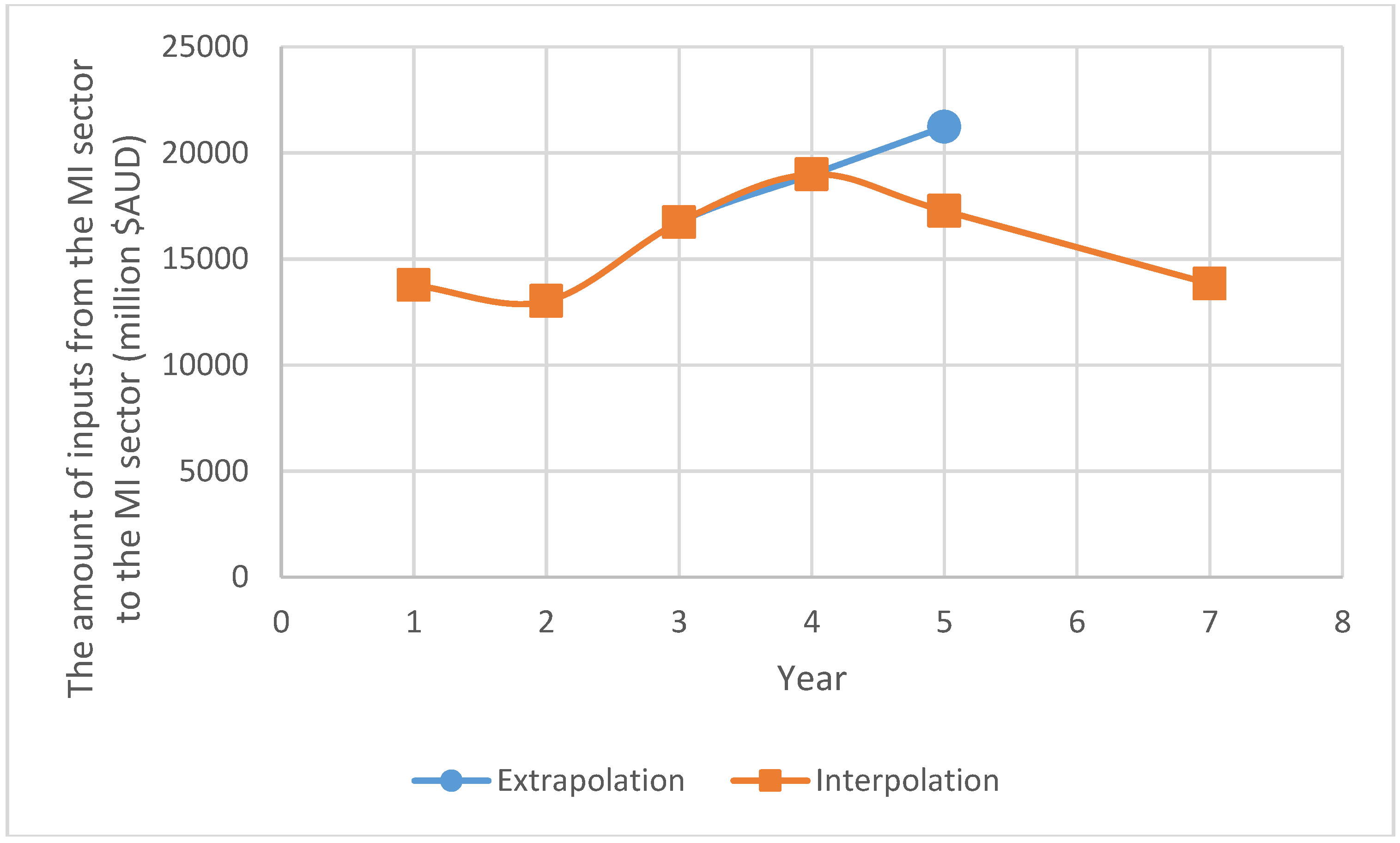
Figure 1.
The comparative analysis for inputs from the MI sector to the MI sector. Mining = MI.
Figure 1.
The comparative analysis for inputs from the MI sector to the MI sector. Mining = MI.
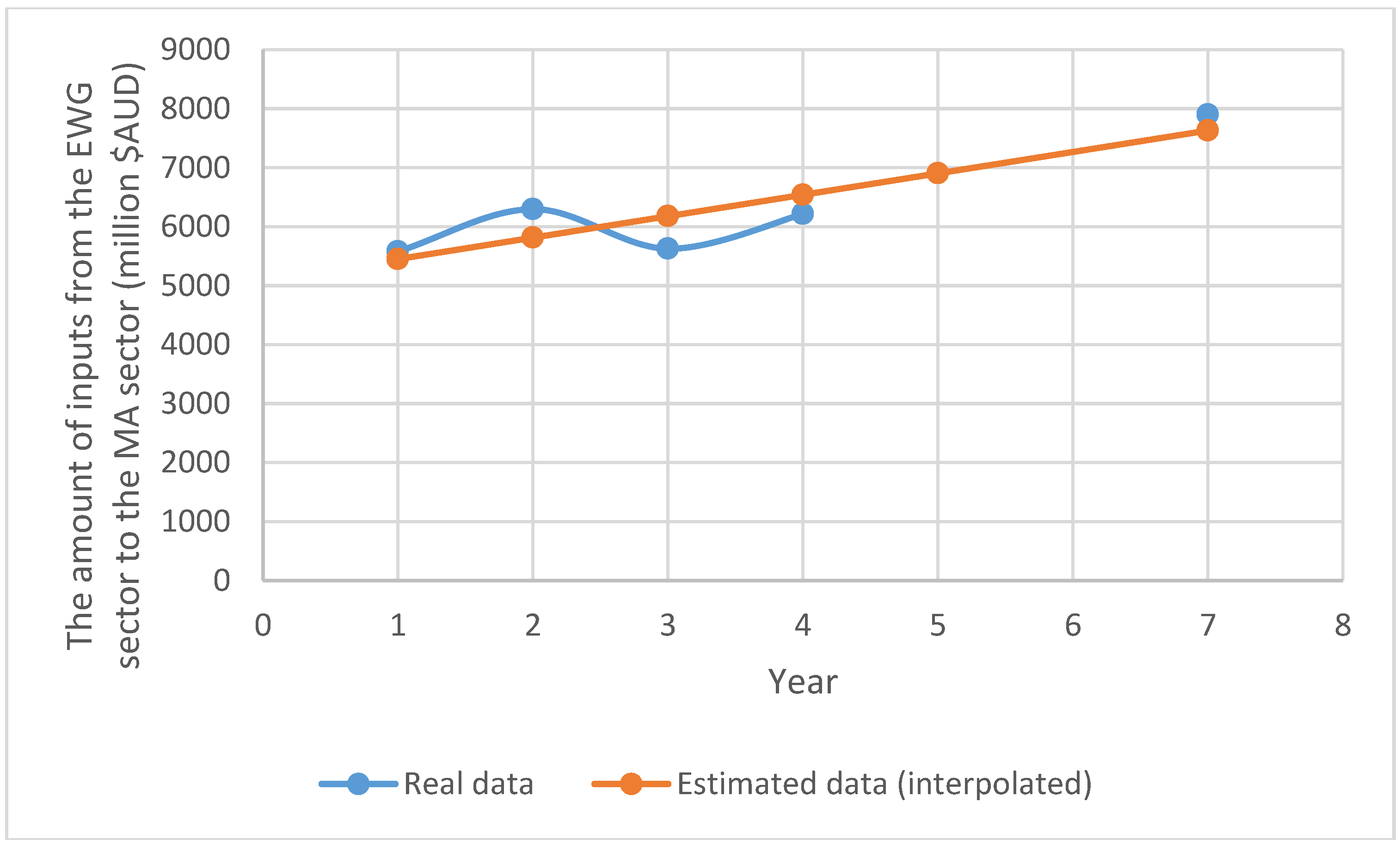
Figure 2.
Inputs from the EWG sector to the MA sector (linear regression equation). Electricity, gas, and water = EGW; Manufacturing = MA.
Figure 2.
Inputs from the EWG sector to the MA sector (linear regression equation). Electricity, gas, and water = EGW; Manufacturing = MA.
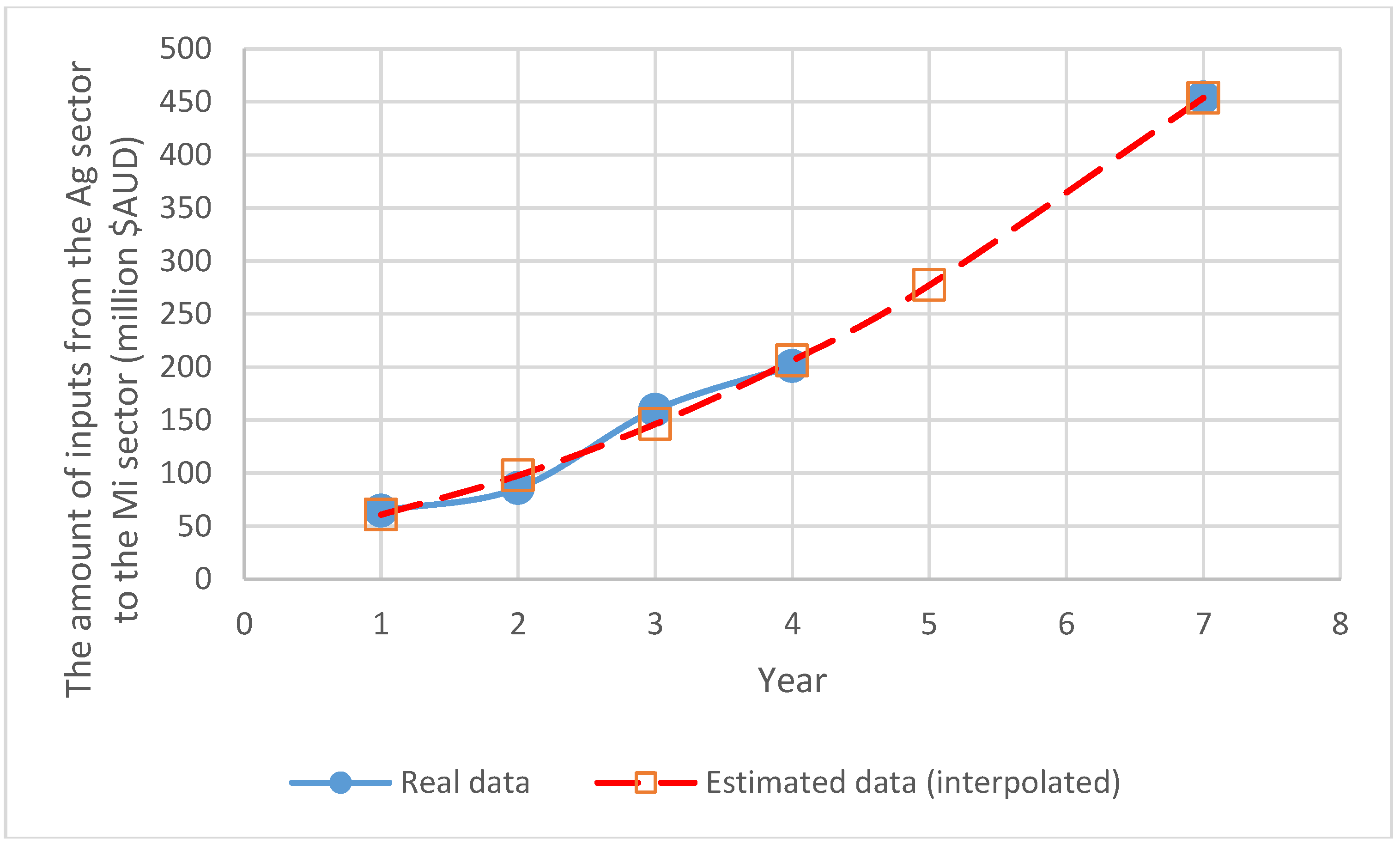
Figure 3.
Inputs from the AG sector to the MI sector (quadratic polynomial equation). Agriculture, forestry, and fishing = AG; Mining = MI.
Figure 3.
Inputs from the AG sector to the MI sector (quadratic polynomial equation). Agriculture, forestry, and fishing = AG; Mining = MI.
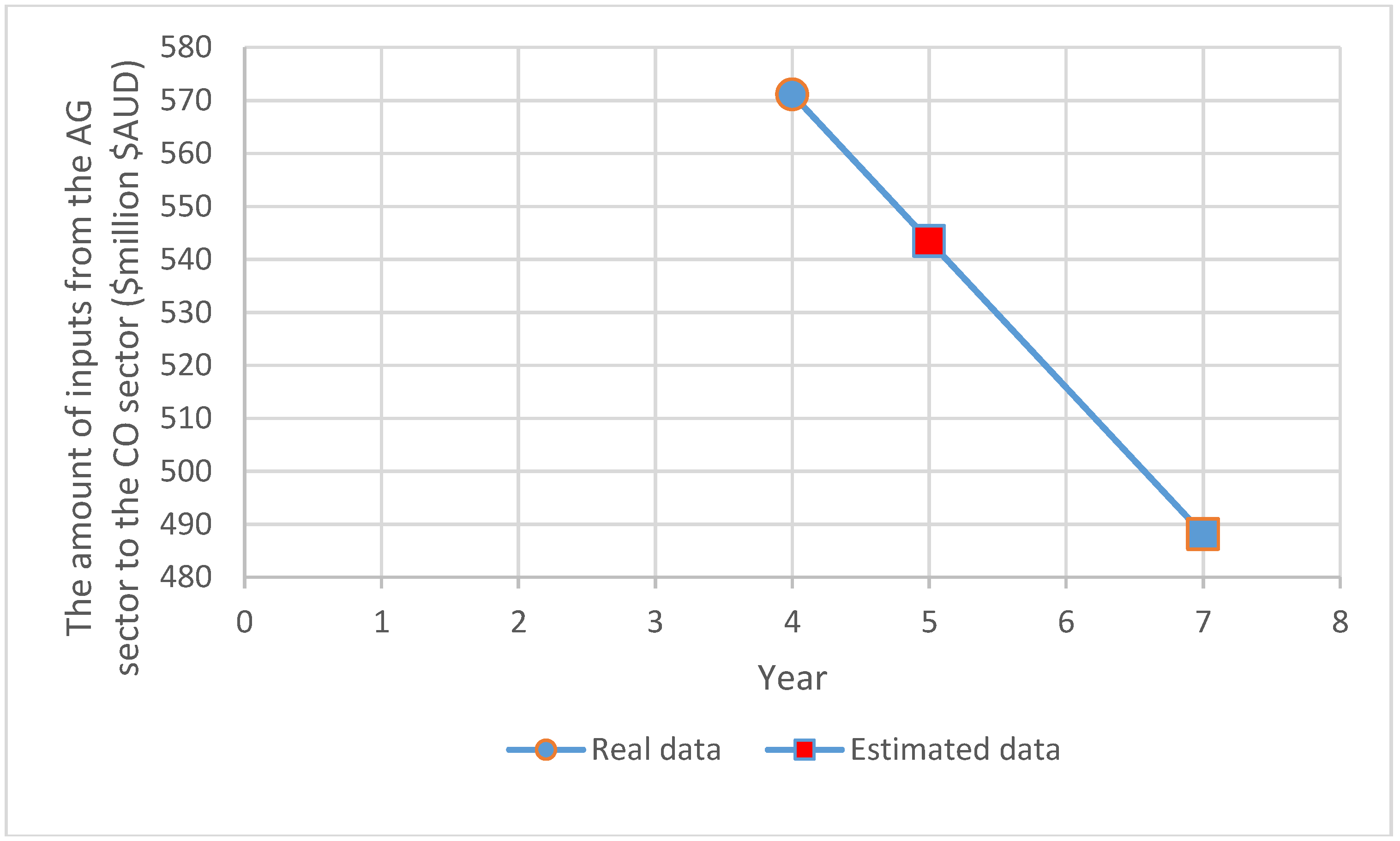
Figure 4.
Inputs from the AG sector to the CO sector in Equation (4). Agriculture, forestry, and fishing = AG; Construction = CO.
Figure 4.
Inputs from the AG sector to the CO sector in Equation (4). Agriculture, forestry, and fishing = AG; Construction = CO.
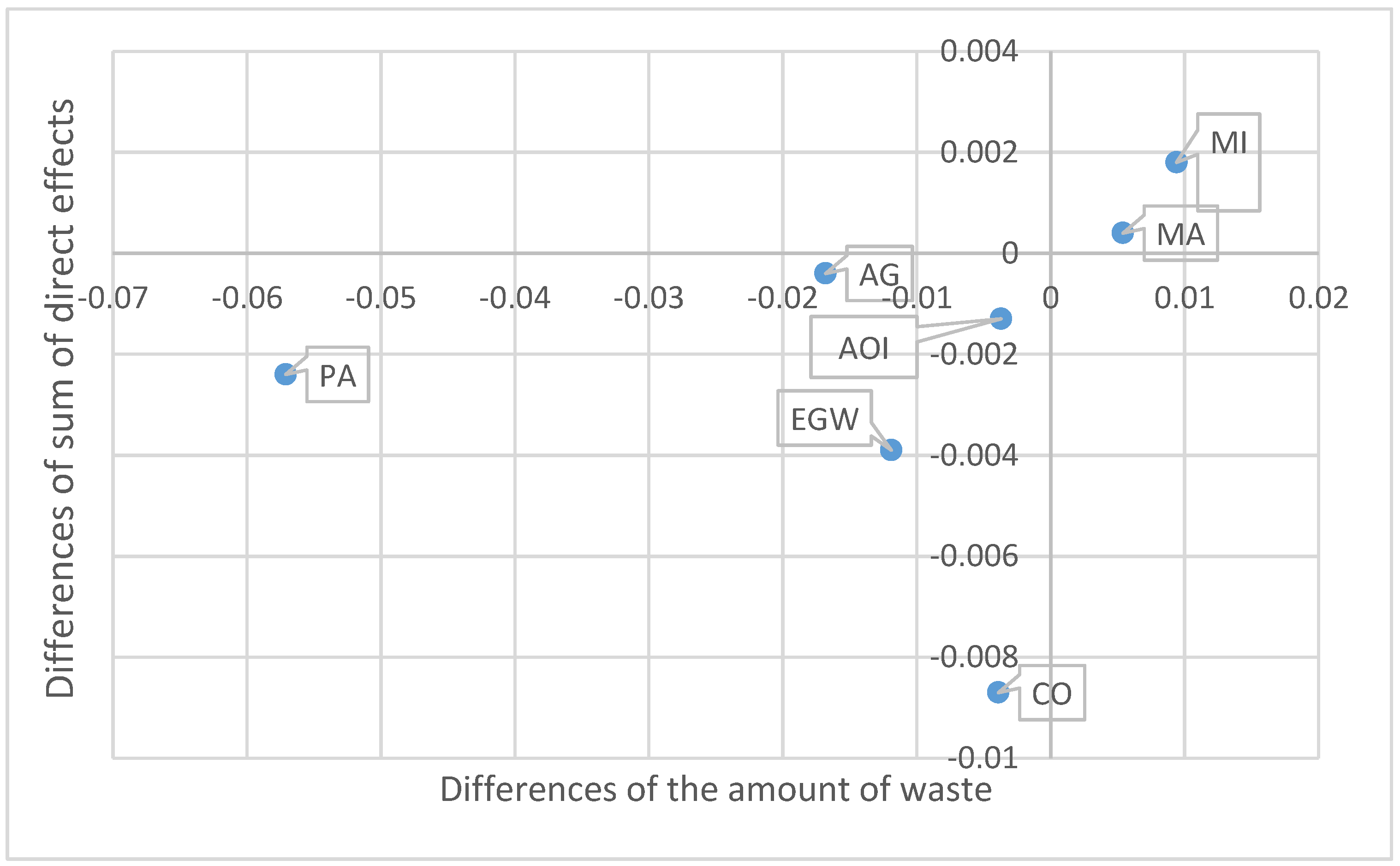
Figure 5.
Relationships between differences of sum of direct effects and the amount of waste generation in various sectors of the Australian economy, YEAR. Agriculture, forestry, and fishing = AG; Mining = MI; Manufacturing = MA; Electricity, gas, and water = EGW; Waste management services = WMS; Construction = CO; Public administration = PA; All other industry = AOI.
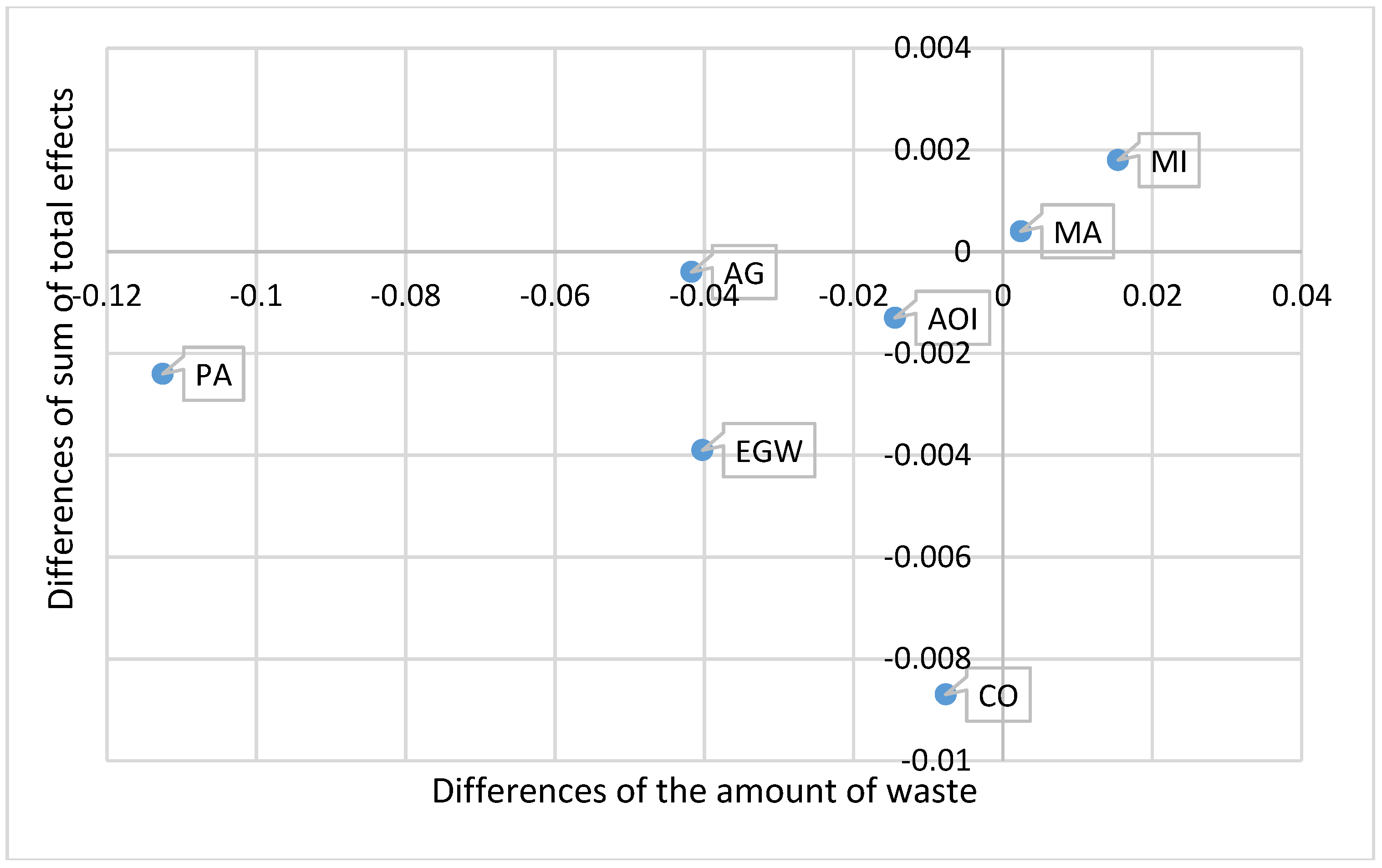
Figure 6.
Relationships between differences of sum of total effects and the amount of waste generation in various sectors of the Australian economy, YEAR. Agriculture, forestry, and fishing = AG; Mining = MI; Manufacturing = MA; Electricity, gas, and water = EGW; Waste management services = WMS; Construction = CO; Public administration = PA; All other industry = AOI.
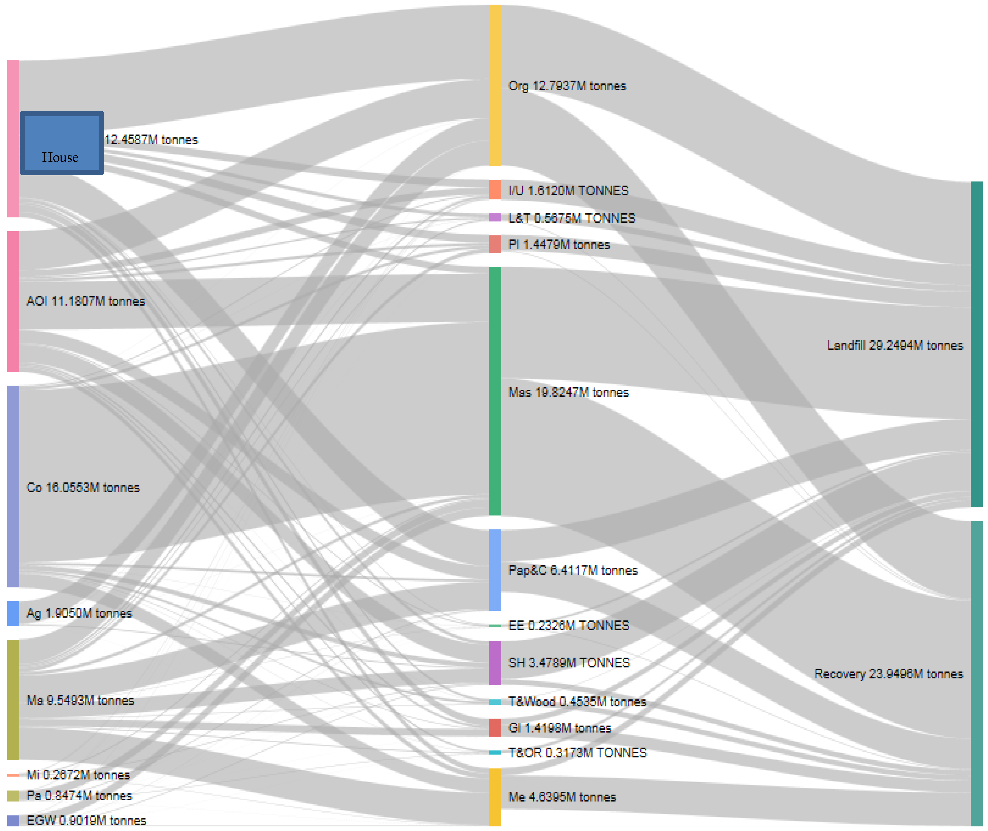
Figure 7.
Physical flow of waste footprints in the Australian WIO table in 2009–2010; waste generated by intermediate sectors (left) and the households (left), sorted into 12 categories (middle), and dealt with by two waste treatment methods (right). Final demand refers to the households. Agriculture, forestry, and fishing = AG; Mining = MI; Manufacturing = MA; Electricity, gas, and water = EGW; Waste management services = WMS; Construction = CO; Public administration = PA; All other industry = AOI.
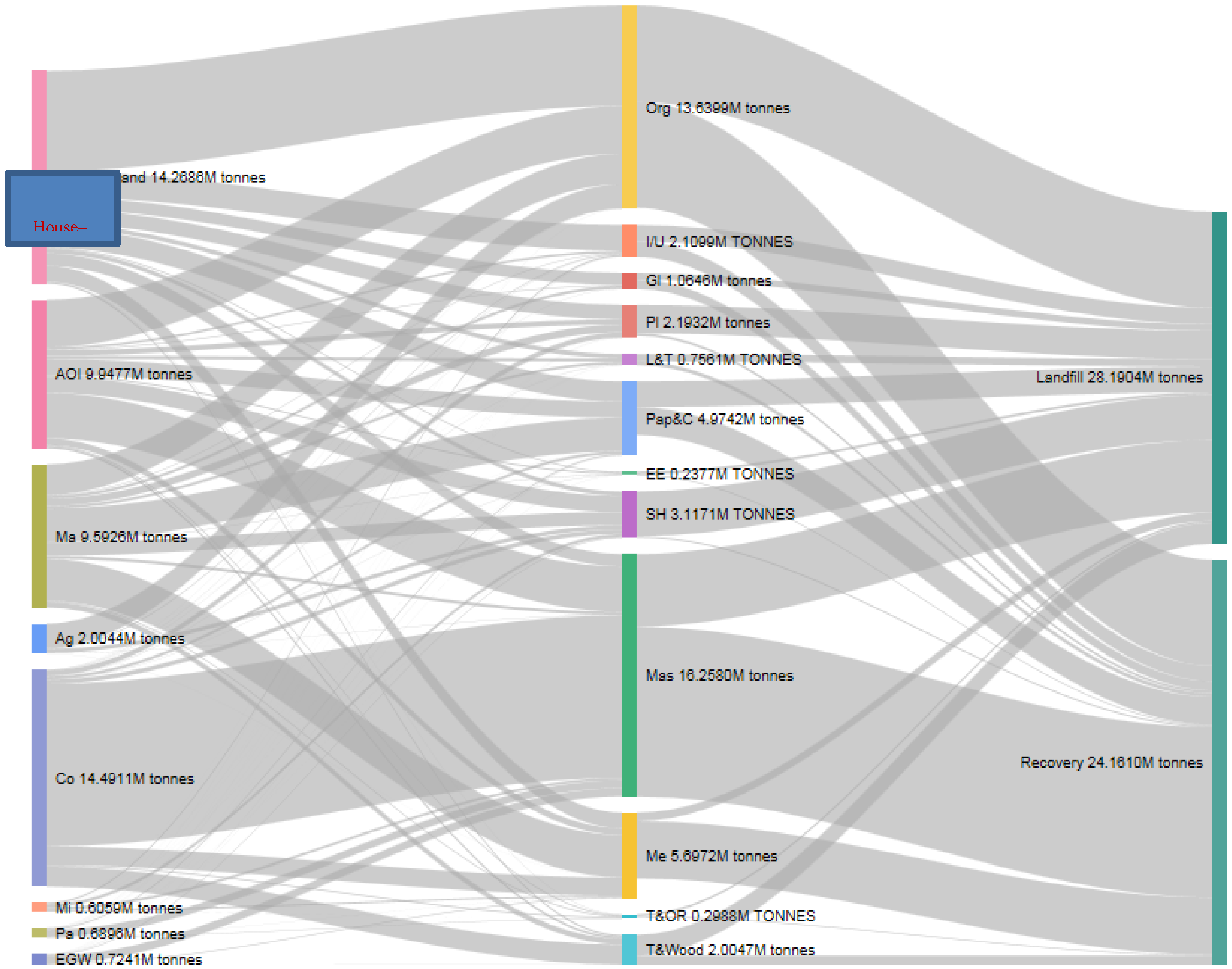
Figure 8.
Physical flow of waste footprints in the Australian waste input output (WIO) table of 2010–2011; waste generated by intermediate sectors (left) and the households (left), sorted into 12 categories (middle), and dealt with by two waste treatment methods (right). Final demand refers to the households. Agriculture, forestry, and fishing = AG; Mining = MI; Manufacturing = MA; Electricity, gas, and water = EGW; Waste management services = WMS; Construction = CO; Public administration = PA; All other industry = AOI.
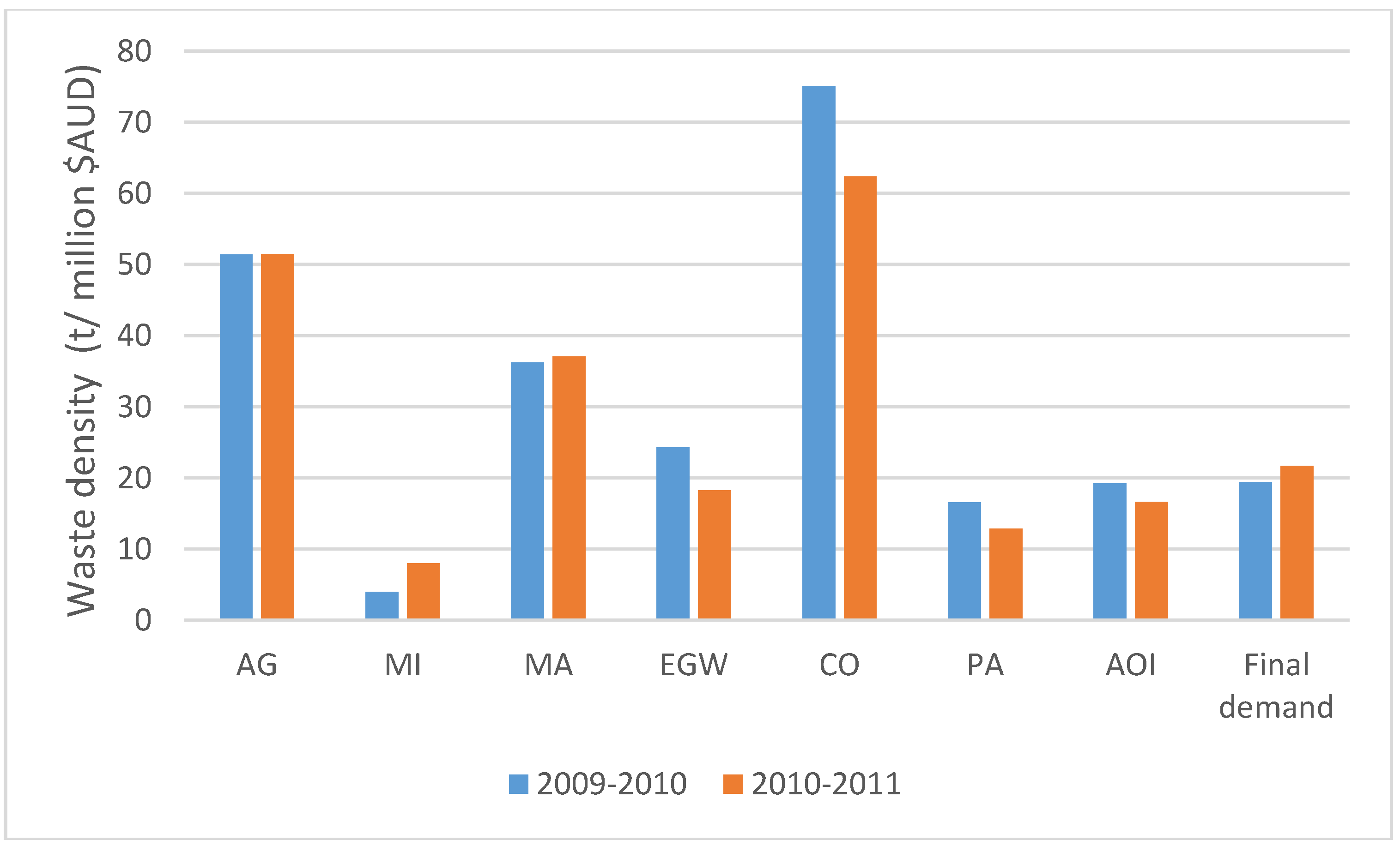
Figure 9.
The waste generation intensity in intermediate sectors and the households in 2009–2010 and 2010−2011, within the Australian economy. Agriculture, forestry, and fishing = AG; Mining = MI; Manufacturing = MA; Electricity, gas, and water = EGW; Waste management services = WMS; Construction = CO; Public administration = PA; All other industry = AOI.
Table 1.
The sector terms and their corresponding abbreviations in the study.
Table 1.
The sector terms and their corresponding abbreviations in the study.
| Terms | Abbreviations |
|---|
| Agriculture, forestry, and fishing | AG |
| Mining | MI |
| Manufacturing | MA |
| Electricity, gas, and water | EGW |
| Waste management services | WMS |
| Construction | CO |
| Public administration | PA |
| All other industry | AOI |
| Paper and cardboard | Pap & C |
| Glass | GL |
| Plastics | PL |
| Metals | ME |
| Organics | Org |
| Masonry | Mas |
| Electrical and electronic waste | EE |
| Solid hazardous waste | SH |
| Leather and textiles | L & T |
| Tyres and other rubber | T & OR |
| Timber and wood products | T & Wood |
| Inseparable/unknown waste | I/U |
| Australian Bureau of Statistics | ABS |
Table 2.
An aggregation waste input-output (WIO) framework based on various sectors of the Australian economy.
Table 2.
An aggregation waste input-output (WIO) framework based on various sectors of the Australian economy.
| | Intermediate Sectors | Treatment Sectors | Final Demand | Total Output |
|---|
| AG | MI | MA | EGW | CO | PA | AOI | Landfill | Recovery | Households |
|---|
| Intermediate sectors | AG | | | | |
| MI |
| MA |
| EGW |
| CO |
| PA |
| AOI |
| Treatment sectors | Landfill | | | | |
| Recovery |
Table 3.
Regression models with their main characteristics for the AOI sector to intermediate sectors using interpolation, coefficients (n = 5).
Table 3.
Regression models with their main characteristics for the AOI sector to intermediate sectors using interpolation, coefficients (n = 5).
| Dependent Variable | Adjusted R2 | p-Value | Independent Variables | Coefficient | p-Value |
|---|
| AOI – AG | | | Constant | 12,020.47 | |
| Year | 157.00 | |
| Year^2 | | |
| AOI – MI | 0.93 | 0.04 | Constant | 16,710.85 | |
| Year | 498.02 | |
| Year^2 | 447.70 | |
| AOI – MA | 0.97 | 0.02 | Constant | 3407.40 | 0.00 |
| Year | −291.97 | 0.01 |
| Year^2 | 16,065.30 | 0.01 |
| AOI – EGW | | | Constant | 1225.05 | |
| Year | 1629.38 | |
| Year^2 | | |
| AOI – CO | 0.97 | 0.02 | Constant | 47,997.12 | 0.00 |
| Year | 9079.35 | 0.02 |
| Year^2 | −826.08 | 0.03 |
| AOI – PA | 1.00 | 0.00 | Constant | 19,642.77 | 0.00 |
| Year | 4131.77 | 0.00 |
| Year^2 | −271.90 | 0.01 |
| AOI – AOI | 0.93 | 0.03 | Constant | 355,732.03 | 0.00 |
| Year | 9864.20 | |
| Year^2 | 1170.11 | |
| AOI – WMS | 0.90 | 0.05 | Constant | 193.38 | |
| Year | 24.58 | |
| Year^2 | 8.96 | |
| AOI – Households | 0.99 | 0.00 | Constant | 397,352.94 | 0.00 |
| Year | 21,404.46 | |
| Year^2 | 1039.74 | |
| AOI – Other final demand | 0.99 | 0.01 | Constant | 210,573.24 | 0.00 |
| Year | 10,616.83 | |
| Year^2 | 59.81 | |
Table 4.
The interpolation of Australian aggregation input-output table (IOT) of 2010–2011.
Table 4.
The interpolation of Australian aggregation input-output table (IOT) of 2010–2011.
| | AG | MI | MA | EGW | CO | PA | AOI | WMS | Households | Other Final Demand | Total Output |
|---|
| (Million $AUD) |
|---|
| AG | 13,881.67 | 277.23 | 24,956.53 | 28.22 | 543.46 | 174.54 | 6054.83 | 0.84 | 6954.43 | 17,070.38 | 69,942.13 |
| MI | 114.39 | 17,264.46 | 33,299.39 | 3115.48 | 2077.38 | 130.89 | 3459.11 | 3.25 | 2276.83 | 117,302.95 | 179,044.12 |
| MA | 5059.59 | 8497.98 | 69,093.36 | 1714.33 | 48,124.90 | 3993.37 | 61,747.67 | 93.42 | 66,304.29 | 104,474.65 | 369,103.56 |
| EGW | 1074.62 | 2813.77 | 6904.17 | 19,755.70 | 1413.32 | 1526.03 | 12,204.49 | 17.43 | 18,074.87 | 7907.22 | 71,691.63 |
| CO | 1348.29 | 8509.97 | 2799.20 | 3882.16 | 90,890.39 | 6384.47 | 29,401.81 | 98.45 | 730.07 | 196,920.53 | 340,965.34 |
| PA | 63.04 | 820.31 | 1327.40 | 153.58 | 1366.49 | 3471.88 | 9116.67 | 2.17 | 1895.53 | 123,398.92 | 141,615.99 |
| AOI | 12,805.48 | 30,393.45 | 68,546.79 | 9371.92 | 72,741.79 | 33,503.98 | 434,305.74 | 540.22 | 530,368.80 | 265,152.52 | 1457,730.69 |
| WMS | 27.33 | 47.77 | 173.65 | 66.99 | 1561.00 | 51.43 | 952.91 | 11.29 | 568.70 | 546.92 | 4007.98 |
| Primary input | 35,567.71 | 110,419.18 | 162,003.06 | 33,603.26 | 122,246.62 | 92,379.40 | 900,487.47 | 3240.92 | 125,292.11 | 87,798.18 | 1673,037.92 |
| Total input | 69,942.13 | 179,044.12 | 369,103.56 | 71,691.63 | 340,965.34 | 141,615.99 | 1457,730.69 | 4007.98 | 752,465.64 | 920,572.28 | 4307,139.37 |
Table 5.
The extrapolation of Australian aggregation input-output table (IOT) of 2010–2011.
Table 5.
The extrapolation of Australian aggregation input-output table (IOT) of 2010–2011.
| | AG | MI | MA | EGW | CO | PA | AOI | WMS | Households | Other Final Demand | Total Output |
|---|
| (Million $AUD) |
|---|
| AG | 15,239.59 | 248.38 | 21,160.68 | 47.56 | 766.92 | 185.10 | 7394.11 | 1.74 | 5834.36 | 12,608.20 | 63,486.64 |
| MI | 50.71 | 21,226.57 | 26,746.83 | 2806.20 | 1942.63 | 136.21 | 3070.96 | 1.31 | 2215.65 | 85,064.27 | 143,261.34 |
| MA | 4468.62 | 5238.63 | 68,817.91 | 1909.33 | 43,217.27 | 3296.43 | 60,070.67 | 90.06 | 70,203.99 | 94,222.78 | 351,535.68 |
| EGW | 1159.01 | 2807.48 | 6800.11 | 21,190.00 | 1322.33 | 676.44 | 12,830.90 | 14.65 | 18,060.18 | 7811.43 | 72,672.53 |
| CO | 749.11 | 8789.97 | 2810.18 | 5887.72 | 88,531.92 | 7827.37 | 33,668.38 | 267.78 | 741.95 | 185,690.64 | 334,965.01 |
| PA | 64.79 | 514.25 | 1443.19 | 179.91 | 1209.16 | 3157.81 | 9018.64 | 1.79 | 1968.98 | 103,499.94 | 121,058.45 |
| AOI | 11,379.83 | 22,194.22 | 69,048.42 | 8762.07 | 76,710.06 | 32,406.08 | 410,306.14 | 352.29 | 523,600.10 | 254,855.82 | 1,409,615.03 |
| WMS | 1.03 | 54.86 | 139.49 | 57.22 | 2306.32 | 34.58 | 324.49 | 0.01 | 782.53 | 424.18 | 4124.73 |
| Primary input | 30,373.95 | 82,186.97 | 154,568.86 | 31,832.52 | 118,958.40 | 73,338.45 | 872,930.74 | 3395.11 | 118,929.80 | 78,648.38 | 1,565,163.17 |
| Total input | 63,486.64 | 14,3261.34 | 351,535.68 | 72,672.53 | 334,965.01 | 121,058.45 | 140,9615.03 | 4124.73 | 742,337.54 | 822,825.63 | 4,065,882.57 |
Table 6.
The Australian waste input output (WIO) table with waste treatment methods, 2009–2010.
Table 6.
The Australian waste input output (WIO) table with waste treatment methods, 2009–2010.
| | AG | MI | MA | EGW | CO | PA | AOI | Landfill | Recovery | Households | Other Final Demand | Total Output |
|---|
| | (Million $AUD) |
| AG | 13,420.64 | 200.87 | 24,772.39 | 34.25 | 571.12 | 175.60 | 6784.67 | 0.57 | 0.43 | 6450.11 | 13,467.36 | 65,878.00 |
| MI | 64.29 | 18,979.43 | 29,647.24 | 3426.72 | 1399.34 | 99.48 | 2826.65 | 0.81 | 0.61 | 2108.02 | 10,3962.42 | 162,515.00 |
| MA | 5099.91 | 7253.39 | 72,764.32 | 1899.70 | 44,135.63 | 4383.00 | 64,633.10 | 58.66 | 44.25 | 67,206.87 | 10,6187.19 | 373,666.00 |
| EGW | 1057.32 | 2499.78 | 6213.25 | 17,311.37 | 1304.40 | 633.32 | 11,422.44 | 7.89 | 5.95 | 16,277.28 | 7493.00 | 64,226.00 |
| CO | 1104.48 | 7569.35 | 3049.72 | 4266.23 | 81,429.02 | 6760.20 | 29,083.91 | 79.18 | 59.74 | 716.71 | 17,9515.46 | 313,634.00 |
| PA | 62.82 | 520.55 | 1275.65 | 150.54 | 1100.35 | 3184.70 | 8717.94 | 1.29 | 0.97 | 1933.61 | 98,802.58 | 115,751.00 |
| AOI | 12,648.48 | 23,691.54 | 69,747.18 | 7742.55 | 71,020.60 | 31,563.06 | 40,4647.88 | 222.25 | 167.67 | 49,7319.66 | 25,1529.13 | 1,370,300.00 |
| Treatment methods | (units: 000 tonnes) |
| Landfill | 1163.69 | 180.45 | 4667.27 | 501.17 | 8205.45 | 475.88 | 6829.83 | 12.09 | 9.00 | 7204.62 | 0 | 29,249.45 |
| Recovery | 741.32 | 86.71 | 4882.03 | 400.75 | 7849.80 | 371.56 | 4350.84 | 7.17 | 5.35 | 5254.03 | 365.03 | 27,602.59 |
Table 7.
The interpolated Australian waste input output (WIO) table with waste treatment methods, 2010–2011.
Table 7.
The interpolated Australian waste input output (WIO) table with waste treatment methods, 2010–2011.
| | AG | MI | MA | EGW | CO | PA | AOI | Landfill | Recovery | Households | Other Final Demand | Total Output |
|---|
| | (Million $AUD) |
| AG | 13,881.67 | 277.23 | 24,956.53 | 28.22 | 543.46 | 174.54 | 6054.83 | 0.48 | 0.36 | 6954.43 | 17,070.38 | 69,942.13 |
| MI | 114.39 | 17,264.46 | 33,299.39 | 3115.48 | 2077.38 | 130.89 | 3459.11 | 1.87 | 1.38 | 2276.83 | 117,302.90 | 179,044.12 |
| MA | 5059.59 | 8497.98 | 69,093.36 | 1714.33 | 48,124.90 | 3993.37 | 61,747.67 | 53.71 | 39.70 | 66,304.29 | 104,474.60 | 369,103.56 |
| EGW | 1074.62 | 2813.77 | 6904.18 | 19,755.70 | 1413.32 | 1526.03 | 12,204.49 | 10.02 | 7.41 | 18,074.87 | 7907.22 | 71,691.63 |
| CO | 1348.29 | 8509.97 | 2799.20 | 3882.16 | 90,890.39 | 6384.47 | 29,401.81 | 56.61 | 41.84 | 730.07 | 196,920.50 | 340,965.34 |
| PA | 63.04 | 820.31 | 1327.41 | 153.58 | 1366.49 | 3471.88 | 9116.67 | 1.25 | 0.92 | 1895.53 | 123,398.90 | 141,615.99 |
| AOI | 12,805.48 | 30,393.45 | 68,546.79 | 9371.92 | 72,741.79 | 33,503.98 | 434,305.70 | 310.63 | 229.59 | 530,368.80 | 265,152.50 | 1457,730.70 |
| Treatment methods | (units: 000 tonnes) |
| Landfill | 1323.11 | 375.42 | 4817.43 | 338.26 | 6781.24 | 322.16 | 5787.22 | 9.00 | 6.67 | 8429.86 | 0.00 | 28,190.37 |
| Recovery | 681.33 | 230.48 | 4775.18 | 385.85 | 7709.83 | 367.39 | 4160.47 | 6.72 | 4.99 | 5838.78 | 3677.05 | 27,838.07 |
Table 8.
The input coefficient matrix of Australian waste input output (WIO) table with waste treatment methods, 2009–2010.
Table 8.
The input coefficient matrix of Australian waste input output (WIO) table with waste treatment methods, 2009–2010.
| | AG | MI | MA | EGW | CO | PA | AOI | Landfill | Recovery |
|---|
| Products and services input coefficients (units: million $AUD per million $AUD of output for intermediate sectors, million $AUD per 1000 tonnes of waste for waste treatment sectors) |
| AG | 0.2037 | 0.0012 | 0.0663 | 0.0005 | 0.0018 | 0.0015 | 0.0050 | 0.0000 | 0.0000 |
| MI | 0.0010 | 0.1168 | 0.0793 | 0.0534 | 0.0045 | 0.0009 | 0.0021 | 0.0000 | 0.0000 |
| MA | 0.0774 | 0.0446 | 0.1947 | 0.0296 | 0.1407 | 0.0379 | 0.0472 | 0.0020 | 0.0016 |
| EGW | 0.0160 | 0.0154 | 0.0166 | 0.2695 | 0.0042 | 0.0055 | 0.0083 | 0.0003 | 0.0002 |
| CO | 0.0168 | 0.0466 | 0.0082 | 0.0664 | 0.2596 | 0.0584 | 0.0212 | 0.0027 | 0.0022 |
| PA | 0.0010 | 0.0032 | 0.0034 | 0.0023 | 0.0035 | 0.0275 | 0.0064 | 0.0000 | 0.0000 |
| AOI | 0.1920 | 0.1458 | 0.1867 | 0.1206 | 0.2264 | 0.2727 | 0.2953 | 0.0076 | 0.0061 |
| Treatment input coefficients (units: 1000 tonnes per million AUS dollar of output for intermediate sectors, 1000 tonnes per 1000 tonnes of waste for waste treatment sectors) |
| Landfill | 0.0177 | 0.0011 | 0.0125 | 0.0078 | 0.0262 | 0.0041 | 0.0050 | 0.0004 | 0.0003 |
| Recovery | 0.0113 | 0.0005 | 0.0131 | 0.0062 | 0.0250 | 0.0032 | 0.0032 | 0.0002 | 0.0002 |
Table 9.
The input coefficient matrix of Australian waste input output (WIO) table with waste treatment methods, 2010–2011.
Table 9.
The input coefficient matrix of Australian waste input output (WIO) table with waste treatment methods, 2010–2011.
| | AG | MI | MA | EGW | CO | PA | AOI | Landfill | Recovery |
|---|
| Products and services input coefficients (units: million $AUD per million $AUD of output for intermediate sectors, million $AUD per 1000 tonnes of waste for waste treatment sectors) |
| AG | 0.1985 | 0.0015 | 0.0676 | 0.0004 | 0.0016 | 0.0012 | 0.0042 | 0.0000 | 0.0000 |
| MI | 0.0016 | 0.0964 | 0.0902 | 0.0435 | 0.0061 | 0.0009 | 0.0024 | 0.0001 | 0.0000 |
| MA | 0.0723 | 0.0475 | 0.1872 | 0.0239 | 0.1411 | 0.0282 | 0.0424 | 0.0019 | 0.0014 |
| EGW | 0.0154 | 0.0157 | 0.0187 | 0.2756 | 0.0041 | 0.0108 | 0.0084 | 0.0004 | 0.0003 |
| CO | 0.0193 | 0.0475 | 0.0076 | 0.0542 | 0.2666 | 0.0451 | 0.0202 | 0.0020 | 0.0015 |
| PA | 0.0009 | 0.0046 | 0.0036 | 0.0021 | 0.0040 | 0.0245 | 0.0063 | 0.0000 | 0.0000 |
| AOI | 0.1831 | 0.1698 | 0.1857 | 0.1307 | 0.2133 | 0.2366 | 0.2979 | 0.0110 | 0.0082 |
| Treatment input coefficients (units: 1000 tonnes per million AUS dollar of output for intermediate sectors, 1000 tonnes per 1000 tonnes of waste for waste treatment sectors) |
| Landfill | 0.0189 | 0.0021 | 0.0131 | 0.0047 | 0.0199 | 0.0023 | 0.0040 | 0.0003 | 0.0002 |
| Recovery | 0.0097 | 0.0013 | 0.0129 | 0.0054 | 0.0226 | 0.0026 | 0.0029 | 0.0002 | 0.0002 |
Table 10.
The Leontief inverse matrix of the Australian waste input output (WIO) analysis, 2009–2010.
Table 10.
The Leontief inverse matrix of the Australian waste input output (WIO) analysis, 2009–2010.
| | AG | MI | MA | EGW | CO | PA | AOI | Landfill | Recovery |
|---|
| (units: million $AUD per million $AUD of output for intermediate sectors, million $AUD per 1000 tonnes of waste for waste treatment sectors) |
| AG | 1.2717 | 0.0121 | 0.1106 | 0.0119 | 0.0297 | 0.0131 | 0.0175 | 0.0005 | 0.0004 |
| MI | 0.0190 | 1.1441 | 0.1198 | 0.0939 | 0.0345 | 0.0122 | 0.0138 | 0.0005 | 0.0004 |
| MA | 0.1577 | 0.0986 | 1.2928 | 0.1016 | 0.2781 | 0.0956 | 0.0984 | 0.0041 | 0.0033 |
| EGW | 0.0370 | 0.0306 | 0.0395 | 1.3782 | 0.0218 | 0.0163 | 0.0201 | 0.0007 | 0.0005 |
| CO | 0.0475 | 0.0853 | 0.0407 | 0.1411 | 1.3750 | 0.0984 | 0.0473 | 0.0042 | 0.0034 |
| PA | 0.0048 | 0.0065 | 0.0080 | 0.0067 | 0.0097 | 1.0321 | 0.0103 | 0.0002 | 0.0001 |
| AOI | 0.4161 | 0.3013 | 0.4207 | 0.3336 | 0.5390 | 0.4654 | 1.4755 | 0.0137 | 0.0109 |
| Treatment input coefficients (units: 1000 tonnes per million AUS dollar of output for intermediate sectors, 1000 tonnes per 1000 tonnes of waste for waste treatment sectors) |
| Landfill | 0.0281 | 0.0067 | 0.0218 | 0.0177 | 0.0429 | 0.0107 | 0.0104 | 1.0007 | 0.0005 |
| Recovery | 0.0191 | 0.0053 | 0.0208 | 0.0147 | 0.0403 | 0.0088 | 0.0075 | 0.0005 | 1.0004 |
Table 11.
The Leontief inverse matrix of the Australian waste input output (WIO) analysis, 2010–2011.
Table 11.
The Leontief inverse matrix of the Australian waste input output (WIO) analysis, 2010–2011.
| | AG | MI | MA | EGW | CO | PA | AOI | Landfill | Recovery |
|---|
| (units: million $AUD per million $AUD of output for intermediate sectors, million $AUD per 1000 tonnes of waste for waste treatment sectors) |
| AG | 1.2620 | 0.0126 | 0.1104 | 0.0100 | 0.0286 | 0.0099 | 0.0152 | 0.0005 | 0.0003 |
| MI | 0.0198 | 1.1197 | 0.1313 | 0.0770 | 0.0392 | 0.0109 | 0.0140 | 0.0006 | 0.0004 |
| MA | 0.1441 | 0.1002 | 1.2784 | 0.0849 | 0.2738 | 0.0722 | 0.0879 | 0.0040 | 0.0030 |
| EGW | 0.0359 | 0.0316 | 0.0435 | 1.3892 | 0.0226 | 0.0227 | 0.0204 | 0.0009 | 0.0006 |
| CO | 0.0499 | 0.0860 | 0.0401 | 0.1185 | 1.3863 | 0.0776 | 0.0450 | 0.0034 | 0.0026 |
| PA | 0.0046 | 0.0082 | 0.0084 | 0.0064 | 0.0103 | 1.0284 | 0.0101 | 0.0002 | 0.0001 |
| AOI | 0.3960 | 0.3355 | 0.4224 | 0.3409 | 0.5193 | 0.3989 | 1.4760 | 0.0183 | 0.0137 |
| Treatment input coefficients (units: 1000 tonnes per million AUS dollar of output for intermediate sectors, 1000 tonnes per 1000 tonnes of waste for waste treatment sectors) |
| Landfill | 0.0286 | 0.0071 | 0.0218 | 0.0117 | 0.0340 | 0.0067 | 0.0083 | 1.0005 | 0.0004 |
| Recovery | 0.0167 | 0.0060 | 0.0202 | 0.0124 | 0.0369 | 0.0067 | 0.0067 | 0.0004 | 1.0003 |
Table 12.
Direct, total, and the change of direct and total effects of sectors on waste treatment method (Landfill) in the Australian economy.
Table 12.
Direct, total, and the change of direct and total effects of sectors on waste treatment method (Landfill) in the Australian economy.
| | Direct Effects | Differences of Direct Effects | Total Effects | Differences of Total Effects |
|---|
| 2009–2010 | 2010–2011 | 2009–2010 | 2010–2011 |
|---|
| (units: 1000 tonnes per million $AUD of output for intermediate sectors) |
| AG | 0.0177 | 0.0189 | 0.0012 | 0.0281 | 0.0286 | 0.0005 |
| MI | 0.0011 | 0.0021 | 0.0010 | 0.0067 | 0.0071 | 0.0004 |
| MA | 0.0125 | 0.0131 | 0.0006 | 0.0218 | 0.0218 | 0.0000 |
| EGW | 0.0078 | 0.0047 | −0.0031 | 0.0177 | 0.0117 | −0.0060 |
| CO | 0.0262 | 0.0199 | −0.0063 | 0.0429 | 0.0340 | −0.0089 |
| PA | 0.0041 | 0.0023 | −0.0018 | 0.0107 | 0.0067 | −0.0040 |
| AOI | 0.0050 | 0.0040 | −0.0010 | 0.0104 | 0.0083 | −0.0021 |
| Sum | 0.0744 | 0.0650 | −0.0094 | 0.1383 | 0.1182 | −0.0201 |
Table 13.
Direct, total, and the change of direct and total effects of sectors on waste treatment method (Recovery) in the Australian economy.
Table 13.
Direct, total, and the change of direct and total effects of sectors on waste treatment method (Recovery) in the Australian economy.
| | Direct Effects | Differences of Direct Effects | Total Effects | Differences of Total Effects |
|---|
| 2009–2010 | 2010–2011 | 2009–2010 | 2010–2011 |
|---|
| (units: 1000 tonnes per million $AUD of output for intermediate sectors) |
| AG | 0.0113 | 0.0097 | −0.0016 | 0.0191 | 0.0167 | −0.0024 |
| MI | 0.0005 | 0.0013 | 0.0008 | 0.0053 | 0.0060 | 0.0007 |
| MA | 0.0131 | 0.0129 | −0.0002 | 0.0208 | 0.0202 | −0.0006 |
| EGW | 0.0062 | 0.0054 | −0.0008 | 0.0147 | 0.0124 | −0.0023 |
| CO | 0.025 | 0.0226 | −0.0024 | 0.0403 | 0.0369 | −0.0034 |
| PA | 0.0032 | 0.0026 | −0.0006 | 0.0088 | 0.0067 | −0.0021 |
| AOI | 0.0032 | 0.0029 | −0.0003 | 0.0075 | 0.0067 | −0.0008 |
| Sum | 0.0625 | 0.0574 | −0.0051 | 0.1165 | 0.1056 | −0.0109 |


