Parameterization and Validation of an Electrochemical Thermal Model of a Lithium-Ion Battery


DLR Institute of Networked Energy Systems, 26123 Oldenburg, Germany
*
Author to whom correspondence should be addressed.
Batteries 2019, 5(3), 62; https://doi.org/10.3390/batteries5030062
Submission received: 15 July 2019
/
Revised: 20 August 2019
/
Accepted: 2 September 2019
/
Published: 6 September 2019
/
Corrected: 23 October 2023
(This article belongs to the Special Issue Thermal Characteristics of Batteries 2019)
Abstract
:The key challenge in developing a physico-chemical model is the model parameterization. The paper presents a strategic model parameterization procedure, parameter values, and a developed model that allows simulating electrochemical and thermal behavior of a commercial lithium-ion battery with high accuracy. Steps taken are the analysis of geometry details by opening a battery cell under argon atmosphere, building upon reference data of similar material compositions, incorporating cell balancing by a quasi-open-circuit-voltage experiment, and adapting the battery models reaction kinetics behavior by comparing experiment and simulation of an electrochemical impedance spectroscopy and hybrid pulse power characterization. The electrochemical-thermal coupled model is established based on COMSOL Multiphysics® platform (Stockholm, Sweden) and validated via experimental methods. The parameterized model was adopted to analyze the heat dissipation sources based on the internal states of the battery at different operation modes. Simulation in the field of thermal management for lithium-ion batteries highly depends on state of charge-related thermal issues of the incorporated cell composition. The electrode balancing is an essential step to be performed in order to address the internal battery states realistically. The individual contribution of the cell components heat dissipation has significant influence on the temperature distribution pattern based on the kinetic and thermodynamic properties.
1. Introduction
Lithium-ion batteries have evolved to be a dependable energy storage technology for mobile and stationary applications due to their high operating voltage and high energy density. To ensure enhanced performance, whilst the applications demand is met, is an increasing challenge on their durability and safety [1,2]. The operating conditions, such as environment temperature, applied current, state of charge (SoC), and mechanical stress within the battery design induce component degradation and can individually or in combination with each other influence the lifetime performance of the battery [3,4,5,6]. Hence, the classification, prediction, and minimization of these stress factors have emerged as important but challenging topics in the field of battery research [7,8,9,10,11].
Different kinds of models were developed to simulate lithium-ion batteries at varying internal states. Simple electrical-circuit models are used to address control strategies within battery management systems. Impedance models are more complex and can be used to map physical processes, which allow for separation of internal physical phenomena and analyzing their dependence on operating conditions. Physico-chemical models are based on fundamental equations describing the migration and diffusion process, as well as the intercalation reaction kinetics within the batteries. Hence, they can be used to understand the impact of changes in material properties on the system’s behavior and improve it. Several papers have been published based on the initial work of Newman and Tiedemann in 1975, and others [12,13,14,15,16]. Further approaches including temperature distributions, first in 2D and later in 3D, are reported in literature [17,18].
However, the key challenge in developing a physico-chemical model is the model parameterization. If conclusions on the battery performance should be drawn based on the internal battery states, the parameter set for the material under consideration is of major importance. Several study approaches have been witnessed on this topic, which range from simple estimations and literature-based parameterization [4,19,20], parameter determination by nonlinear-regression [21,22], to dedicated electrode experiments and full cell evaluation [23,24,25]. The problem with electrode material data is that small changes in the composition and microstructure of the coating can greatly influence the electrode behavior. Electrode performance related to the reaction kinetics is especially problematic, since referenced data is either not available or deviates within several orders of magnitude in comparison to the actual material used [24]. Therefore, several scientific gaps remain to be filled regarding the most appropriate parameterization approach and the accuracy of the model predictions with respect to parameter interdependencies and the model’s application [12].
In this study, a commercially available 40 Ah nickel–manganese–cobalt (NMC) lithium-ion battery cell was selected as the research target, for which no interior construction plan or detailed information on material composition is given. We contribute with this paper by proposing a strategic model parameterization procedure to replicate the heuristic electrical and thermal behavior of the battery, while unrealistic behavior, especially induced at limiting operation modes, is avoided. Four mandatory parameter evaluation groups are identified: “Cell geometry details, thermo-physical properties, cell balancing, and reaction kinetics” and accompanied methods are introduced and executed. The model is established based on the COMSOL Multiphysics® simulation platform and validated via experimental methods. The main advantage of the proposed model is to quickly and non-invasively identify a wide range of parameter values dependent on the choice of operating conditions during the parametrization and thereafter. Finally, the parameterized model was adopted to analyze the heat dissipation sources based on the internal states of the battery.
2. Theory
The conversion and transport theory behind electrochemistry and heat transfer will be introduced from an application-oriented point of view. This model is implemented in the COMSOL Multiphysics® v5.4 environment using the “lithium-ion battery” submodule to describe the electrochemical behavior and an ordinary differential equation to respect heuristic thermal behavior of the battery.
The schematic of the model implemented is shown in Figure 1.
2.1. Lithium Ion Battery
The implementation rests on porous electrode theory, concentrated solution theory, and kinetics equations [12,13,16]. The partial differential equations of the electrochemical and temperature propagation are reported in similar applications [20,26].
The intercalation and de-intercalation processes of the lithium-ions in each electrode are evaluated on the surface of spherical particles (-axis), while the transfer processes are considered unidirectional between the cell layer (-axis). The variables solved within the electrochemical model are the solid-phase lithium-ion particle concentration (), the liquid-phase lithium-ion particle concentration (), the solid-phase potential (), and the liquid-phase potential () [12].
The physical phenomena considered are current and mass conservation in the solid and liquid phase. For the electrodes, Fick’s Law of diffusion for spherical particles is used to derive the solid phase lithium-ion particle concentration (). The determination of the liquid phase lithium-ion particle concentration () is done using mass conservation within the electrolyte in each domain. The derivation of solid-phase potential () in the electrodes is accounted for by Ohm’s law. The calculation of the liquid-phase potential () in the electrolyte is done by using Kirchhoff’s and Ohm’s laws. The calculation of the pore wall flux of the lithium-ions () into the electrodes is performed with help of the Butler–Volmer reactions kinetics equation [12,27].
A complete derivation of the model equations, including initial and continuity conditions, is beyond the scope of the paper. Derivation and discussions of the model type [28,29,30,31] and the implementation in COMSOL Multiphysics® [20] can be found within the reference list.
The governing equations are shown in Table 1. For the sake of simplicity, whenever a parameter is modified with respect to the underlying degrees of freedom, it is denoted by . The phase and domain indices are denoted by and respectively. The parameter definition and parameterization are referred to in Section 5.5.
Heat dissipation sources will be quantified based on the solution variables. The total battery heat dissipation density is implemented in this study as the sum of the integrated heat dissipation sources resulting during energy transfer processes [20,32]. Heat generated by side reactions and particle mixing within the electrode domains is considered negligible [2,33]. The heat dissipation density variable is defined based on [20,31,32] and is shown in Table 2.
The specific parameter definition and parameterization is referred to in Section 5.5.
2.2. Heat Transfer
The following ordinary differential equation accounts for the heuristic temperature calculation and is defined with respect to [34]:
where is temperature, is the external temperature, is the battery density, is the battery heat capacity, is the battery volume, is the total heat dissipation density, is the electrode stack volume, is the battery surface with cooling by convection, is the convective heat transfer coefficient, A is the surface area-dependent effective emissivity, and is the Stefan–Boltzmann constant.
2.3. Coupling of the Physics
The governing equations shown in Table 1 represent the electrochemical behavioral model of the battery with respect to the operations modes: , , and SoC. The total heat dissipation density of the battery with respect to the aforementioned setting is defined in Table 2. In Equation (1) the thermal behavior of the battery is calculated in dependence of the heat dissipated, while simultaneously exchanging the temperature T with the electrochemical variables in the particle, electrode, and electrolyte domains.
3. Experimental Techniques
A model parameterization includes multiple steps: “Opening a battery cell, sample extraction and preparation, measurement execution, and evaluation [23,24,25,35,36].” Special focus was taken on an accurate pre-set of the initial SoC of the battery cell before each measurement objective. The initial SoC of 100% was approached by a 1 C constant current–constant voltage charge to 4.2 V with a cut-off current of C. The initial SoC of 0% was approached by stepwise constant current discharge phases with C, C, C, C, C, and C until the cut-off voltage of 2.8 V was reached. Between each measurement, there was at least two hours’ wait for a full thermal and electrochemical homogenization at the initial state of the test environment.
In this section, measurement techniques used for the battery under investigation are described.
3.1. Battery Description
The commercially available prismatic format (PHEV2) battery used for the model parameterization is labelled to be an NMC/Graphite type with a nominal theoretical capacity of 40 Ah and 144 Wh, measured at C constant current rate. A voltage range between 2.8 V to 4.2 V is recommended with a nominal voltage of 3.6 V. Charging within a temperature range of 0 to 45 °C up to a maximal discharge current rate of 5 C, as well as discharging with 10 C within −10 °C to 65 °C, is approved.
3.2. Pre-Mortem Techniques
The cycling for the electrical measurements was performed by a Maccor series 4000 Potentiostat, multiple cell tester with 0 to 8 V (0.02% accuracy) for voltage and 0 to 150 A current (0.05% accuracy) range each. The climate was controlled by a Vötsch climate chamber, VC 7018 with a temperature range of −75 to 180 °C, and temperature was measured by an Agilent 34972A with PT100 sensors, −40 to 85 °C ( K accuracy) temperature range. The chamber has active air circulation to ensure accurate conditions dependent on each measurement style. The electrical impedance spectroscopy (EIS) was performed by a Solartron Analytical Modulab, XM ECS System, Potentiostat.
3.2.1. Quasi-Open-Circuit Voltage (qOCV)—Low Current Method
The battery was measured during a separated charge and discharge phase with a C rate and a constant temperature environment of 25 °C.
3.2.2. Open-Circuit Voltage (OCV)—Rest Method
The battery was measured during a discharge and a charge phase. Each stepwise discharge of 10% nominal capacity was followed by a break until a voltage change of smaller than 2 mV occurred or 1 h duration was reached. The initial state during the charge phase was the last state of charge during the discharge phase, after relaxation, when a cut-off voltage of 2.8 V was reached.
3.2.3. Electrochemical Impedance Spectroscopy (EIS)
The potentiostatic measurement was performed at the battery at 50% SoC, roughly at 22.5 °C, with 10 mV amplitude and a maximal current of 2 A within a frequency range of 10 mHz to 1 kHz.
3.2.4. Internal Resistance Measurement by Hybrid Pulse Power Characterization (HPPC)
The resistance of the battery within a 3 C discharge pulse for 30 s, measured after 2 s, 10 s, and 18 s, and within a 2 C charge pulse, measured after 10 s, was evaluated at nine different SoCs (10% to 90%), roughly at a temperature of 22.5 °C. After the first and second pulse, a relaxation time of 40 s was performed. Each stepwise discharge of 10% nominal capacity was followed by a break until a voltage change of smaller than 2 mV occurred, or 0.5 h duration was reached.
3.2.5. Electrical/Thermal Validation
Three batteries were measured during separate charge and discharge phases at 0.5 C, 1 C, and 2 C constant current profiles with an initial temperature set to 25 °C. While the battery was charged/discharged, the chambers climate control was turned off to avoid undesired fan cooling. The exterior environment temperature of 22.5 °C and imposed reflective radiation by the chambers interior metal surfaces are assumed to have a negligible effect on the measurement results.
3.3. Post-Mortem Techniques
3.3.1. Cell Opening and Sample Preparation
The battery was opened at a SoC of 0% and an ambient temperature of 22 °C. Due to the possibility of undesired material modification by contact to air, a full disassembly of the battery cell is recommended to be done under argon atmosphere within a glovebox [37]. However, to be able to separate the electrode stack and terminal from the metal casing of the prismatic battery cell, a cut at the top edge of the battery cell was performed first with a Dremel® tool (Racine, WI, USA) under a fume hood [38]. During this process, the batteries’ temperature and voltage were carefully measured. Fast changes would have indicated the activation of electrode stack internal chemical heating processes due to the reaction with air or due to the heating by the cutting process. A voltage drop above 0.1 V or a high temperature increase above 5 K difference did not happen. Thereafter, the lower part of the metal casing could be detached from the terminal and electrode stack carefully with no excessive force.
The final disassembly step of the electrode stack and terminal was done within a glovebox under an inert argon atmosphere on non-conducting ground, atmospheric pressure, and with water and oxygen below 5 ppm. Due to the electrode stack design, a clean cut with a sharp ceramic knife between terminal and stack was executed. This step has to be done with care, however, to avoid cross-contamination or short circuits by metal dust and swarfs between the electrode types. The double-sided electrodes and the separator are detached from each other and stored and sealed in separate containers. In these conditions, the electrode materials quality is not stable, since the material’s fraction of active lithium might still react with small amounts of oxygen or water and electrolyte might evaporate even when the bags are sealed airtight. Therefore, further measurements should be performed within days to avoid the effect of uncertain sample dissipation.
For measurement methods outside the glovebox or when material is intended to be stored for a longer duration, however, a washing process with solvent is recommended to reduce the impact of sample dissipation. The procedure chosen within this study consists of two bathing steps per material sheet with 10 mL pure dimethyl carbonate (DMC) and 1 min duration each, always performed in exactly the same way. The procedure chosen within this study consist of two bathing steps per material sheet with 10 mL pure DMC and 1 min duration each, always performed in exactly the same way [37].
3.3.2. Geometrical Data Measurement
The total thickness of the electrode sheets and the separator were measured with a micrometer-screw at five different points of each material and an average was taken.
X-ray micro-computed (µ-CT, SkyScan 1172, Bruker, Belgium) and nano-computed tomography (-CT, SkyScan 2011, Bruker, Belgium) was used to access the electrodes layer and coating configuration. All tests were done at room temperature with a set voltage of 80 kV for the µ-CT and 40 kV for the -CT. The recorded data sets were reconstructed and selected volume of interest(s) (VOI) and region of interest(s) (ROI) were quantitatively analyzed using associated software products (SkyScan, Bruker, Belgium):
- NRecon: The obtained datasets of recorded images are reconstructed to a 3D cross-Section image stack. The ring artefact and beam hardening values are kept constant for all the samples.
- Data Viewer: The reconstructed images are adjusted parallel to their respective viewing plane, coronal and sagittal, and the VOI is defined.
- CTAn: For the 3D morphometric analysis, the shape and sheet number of ROI are defined.
For the determination of the current collector thickness, the electrode sheets were measured by the µ-CT at a resolution of 1.17 µm/pixel with a rotation step of 0.75° per projection, each projection being an average of four image frames. The 3D reconstructed data set was viewed at coronal and sagittal planes, the thickness was determined at a minimum of ten different points on each plane, and an average was taken.
For the analysis of particle size and porosity percentage, the negative and positive electrode coatings were detached from the current collector foils. The negative electrode coating was measured by the µ-CT with a resolution of 1 µm/pixel and a rotation step of 0.18° per projection, with each projection being an average of six frames, while the positive electrode coating was measured by the n-CT with a resolution of 0.2 µm/pixel and a rotation step of 0.2° per projection, with each projection being an average of four frames. The morphometric analysis was done on the defined VOI and square shaped ROI of 500 µm × 500 µm for the negative electrode coating and ROI of 100 µm × 100 µm for the positive electrode coating.
Scanning electron microscopy (SEM) was utilized to visualize and confirm the particle sizes and homogenization at the electrode’s surfaces. An InLens electron detector and an accelerator voltage of 20 kV were used for both electrode measurements.
3.3.3. Thermal Parameter Measurement
The cell components double coated graphite anode on copper foil, double coated NMC cathode on aluminum foil, and separator of the electrode stack were characterized using differential scanning calorimetry (DSC 204 F1, Netzsch, Germany) to determine their heat capacities .
The DSC device setup and measurement fundamentals for the evaluation of are described in [39]. The anode and cathode coating were scrapped from the copper and aluminum foil using a scalpel. The scrapped samples were loaded and sealed in hermetic aluminum pans. The measurements parameters were defined on the DSC 204 F1 phoenix software (Netzsch, Germany). The measurements were performed from a temperature of 25 °C to 60 °C with a heating rate of 10 K/min. The baseline correction measurement was performed with an empty pan and the calibration measurement with a sapphire standard of 12.73 mg, a thickness of 0.25 mm, and a diameter of 4 mm. The obtained data was loaded onto the proteus analysis software (Netzsch, Germany) for evaluation. A similar application of the methods for the characterization of lithium-ion battery components is shown in [1].
4. Simulation Techniques
The focus in this section is to assess the types of simulation methods that are needed to analyze the design key parameters that define the correlation of the electrode and cell voltage. The determination of the contributing factors on the cell voltage due to the current flow is separated in the following standardized way, as shown in [40]:
Therein represents the cell voltage, is the open circuit voltage without an applied load, is a pure ohmic voltage drop, is a voltage drop due to passivation film or layers on each electrode respectively, are the polarization voltage drops due to interfacial charge-transfer reactions at each electrode, and is a concentration-related effect like particle diffusion, migration, or convection [40]. Each of the different phenomena is reported to occur on different time scales within the battery’s application and deviate dependent on the considered chemistry [40].
At the start, the behavior of the electrode vs. cell balancing ratio is analyzed in Section 5.3, when no current applied. Hence, in Equation (2) is solely defined by the electrode’s contributions:
Afterward, reaction kinetics methods are considered that are able to separate contributing factors on the battery voltage in Section 4.2, when a current is applied. In both sections, a set of subsequent equations is provided that point out modifications for the application in the model.
4.1. Cell and Electrode Examination
The aim within this examination is to find a suitable and realistic representative function of the negative electrode equilibrium potential under the assumption of a known positive electrode equilibrium potential and a measured quasi-equilibrium cell voltage . A similar approach is reported in previous studies [3,25]. The stoichiometry of both electrodes at 100% and 0% SoC (four parameters: , and ) are initially chosen to be the same as in [25]. The following steps one to three are performed to examine the electrode potentials based on the investigated cell SoC:
- The qOCV potential for the cell is measured during a charge and discharge phase to investigate the actual capacity . The OCV potential of the cell is approximated by the average of the qOCV profiles at normalized time, since the overvoltage error is canceled with respect to the direction of the energy transfer:The overvoltage error cancels out with respect to the direction of each energy transfer.
- The positive electrodes potential in dependence of the electrode SoC is chosen to be taken from literature [25]:The positive electrode potential profile is known to show no extreme characteristic slopes in comparison to the negative electrode potential within the mean SoC range.
- By applying Equations (4) and (5) to Equation (3), the negative electrodes potential is calculated as follows:
By shifting and rescaling parts of the electrode potential curves to fit to the difference of the cell potential the parameters and are derived that uniquely define the electrode SoC windows. A shift of the function is happening, when the threshold values for are transformed by the same value, while rescaling of the function is happening, when the difference is altered. The characteristic potential slope S2, which is localized at a theoretical electrode SoC of 50%, is considered as fit criterion to uniquely define the final thresholds values [41]. A discussion of this step and the results is referred to in Section 5.3. The data processing and implementation of the potential profiles is referred to in Appendix A.
Based on the SoC thresholds of the electrodes and with respect to the maximal lithium particle concentrations of each electrode, the following equations are established with respect to ideas of [28,36] and can be used to define the initial lithium particle concentration of the electrodes at the initial state of charge :
The upcoming set of equations are derived and used to reproduce the design specification of the full cell based on the electrode’s properties () and are used similarly by [23,24,25]:
- The inactive fraction of the electrodes SoC windows is calculated by:
- The actual electrode capacities and are calculated based on the fact that the usable capacity represents the active material loading, while the counterparts in each electrode remain inactive:
- The theoretical electrode capacities are calculated as follows:
- The electrodes active material fraction is received by calculating the ratio of the actual electrode capacity of the theoretical electrode capacity:
- The specific surface area is calculated as follows:
- Similarly, the actual surface area is calculated as follows:
The final results are reported in Table 6 in Section 5.5.
4.2. Reaction Kinetics Examination
Several studies reported on EIS experiments of lithium-ion batteries and half-cells to evaluate cell performance, as shown in Equation (2), and employed the method as reliable to separate the dynamic effects based on the measured impedance response [25,40,42,43,44,45,46]. A small sinusoidal current signal is imposed on the battery at a given frequency and induces a sinusoidal voltage response. Using complex numbers to represent the sinusoidal current and voltage, the complex impedance of the battery at a given frequency can be calculated as follows:
In fact, two characteristic points and corresponding resistance values will be assessed that roughly describe the dynamic behavior of the battery [46]:
- : The impedance spectrum crosses the -axis at the frequency, when the inductive behavior is compensated by capacitive behavior of battery components. Hence, the battery impedance at this point is nearly the pure ohmic resistance of the battery.
- : The negative imaginary part of the impedance spectrum shows a local minimum at the end of a large semicircle at low frequencies. The semicircle is usually associated with interfacial charge transfer reaction combined with double layer capacitance.
The entire impedance spectrum of the battery is evaluated based on the frequencies in the given frequency range 1000 Hz to 0.01 Hz, when a sinusoidal voltage response with 10 mV is produced. The COMSOL Multiphysics® physico-chemical modeling approach [45,47] will be introduced based on the model study one needs to perform to evaluate equation (15). The model study is a stationary frequency analysis and requires modifications of the governing equations:
- The time-dependent model variables, here represented by , are modified by a sinusoidal perturbation and solved in the complex-valued domain for predefined frequencies
- Where is the initial time-dependent value at time zero and is the complex-valued extension of . The particle concentration time derivative mentioned in Table 1 is exchanged by a frequency mode as follows:where incorporates the double layer capacitance at each electrode:Correspondingly, instead of in the governing equations in Table 1.
- Thus, the cell impedance is calculated dependent on the perturbed boundary flux variables and and incorporated conditions defined at the positive current collector:Therein and are a resistance and inductance component, is equal to the applied current density in the solid domain, is the potential within the solid domain, and are the initial time-dependent values at time zero, is the normal boundary flux vector, is the amplitude of the potential perturbation and is the amplitude of the current perturbation induced by .
The model results are initiated based on reference values [25] and refined with respect to the EIS experiment at cell SoC 50% and temperature at 25 °C. The final fitting results are shown in Table 6 in Section 5.5.
For the characterization of low frequency battery dynamics, a HPPC experiment and simulation is considered, as suggested in literature [48,49]. The pulse methodology is not able to separate dynamic contributing factors to the internal resistance value, but it is able to show its evolution and is considered to be the more standardized way in present battery diagnostics and scientific evaluations [40]. To analyze the internal resistance progression at multiple time constants and different SoC levels, the internal resistance is evaluated as the battery’s voltage response of a constant current pulse during a discharge and charge phase:
where is time, is the voltage measured at time is the voltage measured the pulse initiation, and is the applied current.
The following set of equations were chosen and partially refined to reproduce the reaction kinetics of the cell with respect to the governing equations and underlying domains defined in Table 1:
- The temperature dependence of model variables is considered by applying the Arrhenius relation as considered in [25]:where is the variable, is the variables value at the reference temperature , is the activation energy, is the universal gas constant, and is the temperature variable.
- Each electrode’s exchange current density is defined temperature-dependent with respect to [25]:
- Each electrode’s diffusion coefficient is dependent on the electrodes SoC and temperature. Therefore, the following equations are defined with respect to [25]:whereand
- The Li+ transference number is defined as follows, as taken from [50]:
- The effective diffusional electrolyte conductivity is defined as follows, similar to [3]:
The final results are reported in Table 6 in Section 5.5.
4.3. Thermal Behaviour Examination
Effective parameter sets for the density and heat capacity are considered with respect to the geometry of the cell and are calculated based on volume, averaging similar to [1]. Therefore, the geometry was reconstructed based on volumetric measurements of each material component of the battery cell:
where is the volume fraction, is the density, and is the heat capacity of the -th material component of the battery cell.
Convective cooling by air is considered material-independent and the surface area is simply the sum of each material surfaces exposed to air. Cooling by radiation, however, is dependent on the materials surface emissivity. Therefore, the effective emissivity is calculated as follows:
where is the surface-area dependent emissivity, is a surface with applied cooling by radiation, and is the -th material emissivity.
The final results are reported in Table 6 in Section 5.5.
5. Results and Discussion
In this section, the experimental characterization results and evaluated key parameters are gathered and incorporated into the simulation model of the commercially available 40 Ah battery cell. It is investigated how the electrodes balancing and reaction kinetics related phenomena can be derived from full cell measurements and used to define the electrodes characteristics. The simulations are compared with validation experiments to evaluate the electrical and thermal model behavior under the influence of simulated heat dissipation.
5.1. Electrode Geometry Evaluation
The geometry parameters presented in this section are analyzed by post-mortem analysis of the commercial battery cell. The experimental procedures undertaken for this step are explained in Section 3.3.
Based on the material analysis by SEM and data sheet description of the manufacturer, the negative electrode is considered to be graphite, while the material of the positive electrode is supposed to be of the NMC class. The negative electrode consists of flake-shaped particles and the positive electrode consists of agglomerates of smaller particle types as shown in SEM pictures in Figure 2:
The electrode stack of the battery cell is constructed based on a z-folding of the separator with each electrode contained within the folds in alternate order. All electrode sheets are double-coated, even the exterior negative electrode sheets, although no counter electrode is present. Only the interior electrode area is considered to be electrochemically active, therefore the electrode surface area with counter electrode is chosen to be used for the parameterization. Electrodes material properties considered for the parameterization are the thicknesses, particles sizes, and the porosities. The coating thickness is recalculated based on the current collector thickness. The evaluated geometry properties are listed in Table 3.
5.2. Battery Thermal Parameter Examination
Within each component of the battery, thermo-physical properties are different; hence, each component has to be taken into account. The thermal parameters for the battery are listed in Table 4.
The obtained values for the single components are in good agreement with data reported for a NMC/Graphite battery [2]. Temperature dependence of the heat capacity is not considered for the model parameterization, since the analysis of the cell sheet components have shown almost constant behavior within the range from 25 °C to 60 °C. Therefore, the mean value is taken instead.
5.3. Cell Balancing Evaluation
The purpose of the cell balancing evaluation is to access electrode SoC and cell SoC vice versa for SoC-dependent model application and evaluation.
The capacity in the qOCV-experiment during the discharge-phase is Ah and during the charge-phase is Ah. The measured capacity difference of 0.5 Ah might be attributed to one of the following reasons:
- Due to the difficulty to set up the initial cell SoC at 0%, as described in Section 3.2, an off-set within the experiment is realistic.
- An overhang effect at the negative electrode during a prior charge-phase lead to an increased discharge capacity after relaxation [54].
Since this effect is not reproducible with this model type, the cell capacity is defined based on the discharge phase result.
The existence of characteristic potential slopes in the interim SoC range of the full cell are reported to occur within the Graphite OCV profile rather than the positive electrode of different Graphite/Li-Metal-Oxides [23,25,41]. A typical graphite electrodes OCV profile shows several potential slopes dependent of the SoC stages. This is caused by the structure of graphite, where the lithium intercalation between the graphene layers occurs in an ordered pattern [41,55]. The potential profiles for the cell balancing evaluation, a simulation variant, and an experimentally determined OCV profile by rest method are shown for comparison with the suggested lithiation stages within the calculated graphite electrode OCV profile in Figure 3:
The lithium distribution is numerated by a stage number, which indicates the number of graphene layers between the layers of intercalated lithium. Areas of coexisting intercalation phases are seen as plateaus and single-phase areas as change in potential. The intercalation stages are named with an increase in lithium-ion concentration as follows: dilute stage-1 (S1’), stage-4 (S4), stage-3 (S3), liquid-like-stage 2 (S2L), ordered-stage-2 (S2), and ordered stage-1 (S1) [41,56]. S2 is considered as characteristic potential change for the electrode SoC threshold evaluation, since it is located at the theoretical electrode SoC of 50% [25,56,57].
5.4. Reaction Kinetics Evaluation
By fitting the experimental EIS results at cell SoC 50% and temperature 25 °C, the initial electrode exchange current densities taken from [25] are updated.
The Nyquist plot obtained from the experiment and the cell impedance model are shown together, with each contributing impedance part in the frequency domain in Figure 4.
Three different processes with the identified frequency ranges are annotated in Figure 4a: region : 100 Hz up to 1000 Hz, region : 1 Hz up to 100 Hz, and region : 0.01 Hz up to 1 Hz. Each region is reported to coincide with a separate underlying physical phenomenon: experimental test-setup (region ), charge-transfer processes (Region ), and diffusion processes (region ) [58]. In region , an inductive component is existent. A deviation between the simulation and the experiment results is visible. The combination of an inductive component connected in series with a resistance is not able to reproduce the slope of the experimental pattern. The effect however can be interpreted as measurement artifacts that originate from connections at high frequencies and might be attributed to the wiring of the experimental test setup and not necessarily to the battery cell [59].
The semicircle of the charge transfer region is fully resolved and can be fitted to derive values for the reaction rate constants and their double layer capacitances. [43].
The diffusion process within region cannot be fully analyzed due to the limitations in the frequency range of the experimental setup below Hz. Hence, a diffusion-induced contribution on the cells internal resistance will be evaluated based on the pulse methodology. The absolute mean errors for the fitting procedure are shown in Figure 4b,c. The refined values are denoted in Table 6 in Section 5.5.
The evaluation of the HPPC test of the internal resistance is performed based on Equation (22). In Figure 5, mean experimental results and deviations of four different battery cells of the same kind are compared against the simulation results of the battery that is considered for the model’s parameterization.
The general trend visible is an increase of the internal resistance with an increasing time constant to at all SoC levels during the discharge and charge pulse in the simulation and in the experiment. By comparing the magnitude of within the EIS experiment in Figure 4 at the SoC level 0.5 and temperature 25 °C, it can be concluded that the internal resistance value already comprises the ohmic resistance, the complete charge-transfer-resistance, and parts of the diffusion resistance. Hence, the resistance increases between and within the considered temperature regime can mainly be attributed to the effect of electrolyte salt diffusion and electrode diffusion [40,59,60].
At the SoC 0.1, the experimental resistance values are increased at all time constants within comparison to the SoC window . Similarly, the mean error within the SoC window is increased in comparison to the SoC 0.1.The simulation results are located within the error margin of the experimental results in Figure 5a and remain close to or within the error margin in Figure 5b,c. Two distinct peaks are visible within the simulation results that are located at each time constant within the SoC range 0.1 to 0.4 and 0.6 to 0.8, called peak one and peak two, respectively. Their location coincides with the potential slopes due to the structural changes of S4 and S2 within the negatives electrode, as seen in Figure 3. A shift of the peak might be attributed to a SoC change during the applied pulse profile.
The peaks, although heavily shaved, are also visible within the experimental results, around the peaks SoC windows. There are two major reasons that would indicate a peak shaving behavior within the experimental result:
- Each nominal SoC level of the batteries could comprise a deviation in their real capacity that cannot be captured by the experiment setup.
- Each battery contains ninety cells gathered in a parallelized electrode stack. Non-uniformity of the cell SoCs within the stack would indicate a variation in duration and time until the slopes S2 or S4 are passed. Since the batteries’ internal resistance comprises the contributions of each of the cell’s contribution, a slight shift within the peak’s potential would shave the peak magnitude and move its location.
The model is not capable of reproducing the peak shaving behavior, since only one cell sheet is considered; however, the model accurately predicts the increase of the internal resistance dependent on the Cell SoC within comparable magnitude.
5.5. Model Parameterization
In the following, the model’s setup is demonstrated.
5.6. Cell Voltage Validation
The model validation considers both electrochemical and thermal properties. The experimental test procedures considered electrochemical and thermal constant current tests, as described in Section 3.2. For electrical validation, both the voltage curves during a 0.5 C, 1 C, and 2 C discharge and charge phases were taken into account, as shown in Figure 6a–f. The simulated curves match well with the experimental curve and show a relative error within 1% deviation.
More pronounced deviations are visible at the end of the discharge phase and at the beginning of the charge phase. These regions are correlated with a low SoC of the negative electrode and a high SoC of the positive electrode.
5.7. Temperature Validation
For the thermal validation, both the temperature curves during a 0.5 C, 1 C, and 2 C discharge and charge phases were taken into account. The experiments were conducted as mentioned in Section 3.2. The battery temperature was measured by fourteen thermocouples, positioned at different locations on the batteries surface. The average battery temperature and maximal temperature variability of the experiment were compared with the simulation as shown in Figure 7a–f:
The range within the variability of the experimental values and the simulation are basically the same at each constant current rate. However, the relative error increases from 0.5 C to 2 C and the model tends to overestimate the experimental results at elevated current rates. The deviations between the experimental and the simulated temperature values might be attributed to one of the three upcoming reasons:
- No spatial resolution of the battery cell is considered. Hence, no thermal gradient based on the interior cell component connection is created.
- The environment conditions of the battery could affect the experimental results. The climate chamber was turned off, when the experiment was initialized at a constant temperature to prevent weak forced cooling, but fluctuations could still arise by the buoyancy effect within air [64]. The wires and fastener connected to the battery cell could influence the experimental thermal behavior of the battery cell by inducing a thermal outflow [2].
5.8. The Effect of Heat Dissipation on Thermal Behaviour
The heat dissipation sources resulting from effects from each layer and the current collectors within the electrochemical model are categorized into two categories: reversible heat , originated from entropy change of the electrode materials, and irreversible heat, divided into polarization heat and ohmic heat. The simulated heat dissipation densities and temperature curves during 0.5 C, 1 C, and 2 C discharge and charge phases are simulated and shown in Figure 8a–f:
The total heat dissipation is visible as sum of the several contributions. The hatched area depicts compensated dissipation by the mix of endothermic and exothermic heat sources.
The irreversible ohmic heat is almost constant at each C-rate, independent of the charge or discharge direction, and increases from 0.5 C to 2 C practically 15 times.
The irreversible polarization heat has two characteristic peaks within the interims SoC and increases at SoC below 10% significantly at all current rates. The peaks are shifted from their original location at 0.5 C dependent on the charge and discharge direction. They grow and widen with increased current rate up to 15 times their original magnitude. The existence and origin of the peaks is discussed in Section 5.4 based on the resistance evaluation.
The reversible heat dissipation comprises the electrodes entropy profiles [32,63]. The SoC-dependency in this study, however, solely originated from the negative electrode, since the NMC-based electrodes contribution is assumed to be constant [63]. The reversible heat source acts as a coolant at low current SoC during the charge phase and at the interims SoC range during the discharge phase. The first case is reported to correlate to a transition between ordered and disordered states, while the second case is correlated to the transition between the stages S2L and S2 within the lithiation of the negative electrode, as mentioned in Section 5.3.
With increasing current rate, irreversible heat dissipation is dominant. The result is represented by the fact that the characteristic thermal pattern, which is originated from reversible heat dissipation, almost vanished at the 2 C rate; both visible in the simulation and in the experiments.
6. Conclusions
The strategic model parameterization procedure and the developed model established in this study allow simulating electrochemical and thermal behavior of a commercial lithium-ion battery cell with high accuracy.
This work shows that commercially available battery cell models can be parametrized by a sophisticated mixture of material characterization, literature review, and model refinement. This has been confirmed by multiple experimental characterization approaches focused on the battery cell at hand. The hierarchical model parameterization procedure starting from geometry details, incorporating cell balancing and adapting the model to reaction kinetics behavior might be applied by other model developers as well, when data of the considered electrodes are not available.
Under consideration of the heuristic battery thermal properties, this model has proven to be a trustworthy tool to investigate the heat dissipation during diverse battery operation modes. It could be confirmed that the thermal behavior of the battery cell at lower current rates is dominated by reversible heat dissipation. With increasing current rates, a shift towards the dominance of irreversible heat dissipation has been profound.
Author Contributions
Conceptualization, G.L., F.S., and C.A.; Data curation, G.L. and G.G.; Formal analysis, G.L.; Funding acquisition, F.S.; Investigation, G.L., G.G., and U.K.; Methodology, G.L.; Project administration, U.K. and F.S.; Resources, U.K. and F.S.; Software, G.L.; Supervision, C.A.; Validation, G.L. and G.G.; Visualization, G.L.; Writing—original draft, G.L.; Writing—review and editing, G.G., U.K., F.S., and C.A.
Funding
This research “BaSyMo” (FKZ: 03ET6087I) was funded by the Federal Ministry of Economic Affairs and Energy (BMWi).
Acknowledgments
The authors gratefully acknowledge the financial support provided by BMWi, the German Federal Ministry of Economic Affairs and Energy, for funding of the project BaSyMo (FKZ: 03ET6087I). We like to thank our project partner for their excellent collaboration on the topic of battery research: ElringKlinger AG. The authors thank O. Zahid for the geometric characterization of the commercial battery cell and the derived thermal parameters, the properties of which were further investigated in this study by numerical analysis.
Conflicts of Interest
The authors declare no conflict of interest. The founding sponsors had no role in the design of the study; in the collection, analyses, or interpretation of data; in the writing of the manuscript, and in the decision to publish the results.
Appendix A
OCV Profiles
For the use of interpolated functions within COMSOL Multiphysics®, a reduced set of nodes and corresponding function values are required. Within the simulation platform, the piecewise cubic interpolation method is considered within the node interpolation functions. The method generates a Hermite polynomial , index set, which preserves the shape of the data, respects monotonicity, and has a continuous first derivative. The interpolation values of the positive electrode profile are created based on the coefficient data taken from literature [25]. The derivation of the negative electrode profile is described in Section 4.1.

Table A1.
Values of the interpolation nodes of the electrode equilibrium potential profiles.
| 0.0100 | 0.8391 | 0.4150 | 4.2754 |
| 0.0178 | 0.6452 | 0.4204 | 4.2626 |
| 0.0255 | 0.5368 | 0.4258 | 4.2497 |
| 0.0333 | 0.4587 | 0.4312 | 4.2369 |
| 0.0410 | 0.3983 | 0.4366 | 4.2242 |
| 0.0488 | 0.3493 | 0.4420 | 4.2116 |
| 0.0565 | 0.3082 | 0.4474 | 4.1993 |
| 0.0643 | 0.2736 | 0.4528 | 4.1873 |
| 0.0720 | 0.2447 | 0.4582 | 4.1754 |
| 0.0798 | 0.2271 | 0.4636 | 4.1636 |
| 0.0875 | 0.2226 | 0.4690 | 4.1519 |
| 0.0953 | 0.2211 | 0.4744 | 4.1404 |
| 0.1030 | 0.2200 | 0.4798 | 4.1290 |
| 0.1108 | 0.2190 | 0.4852 | 4.1177 |
| 0.1185 | 0.2178 | 0.4906 | 4.1066 |
| 0.1263 | 0.2163 | 0.4960 | 4.0956 |
| 0.1340 | 0.2142 | 0.5014 | 4.0847 |
| 0.1418 | 0.2114 | 0.5068 | 4.0739 |
| 0.1495 | 0.2070 | 0.5122 | 4.0633 |
| 0.1573 | 0.2007 | 0.5176 | 4.0527 |
| 0.1650 | 0.1941 | 0.5230 | 4.0423 |
| 0.1728 | 0.1884 | 0.5284 | 4.0320 |
| 0.1805 | 0.1821 | 0.5338 | 4.0219 |
| 0.1883 | 0.1754 | 0.5392 | 4.0119 |
| 0.1960 | 0.1699 | 0.5446 | 4.0022 |
| 0.2038 | 0.1658 | 0.5500 | 3.9926 |
| 0.2115 | 0.1617 | 0.5554 | 3.9832 |
| 0.2193 | 0.1574 | 0.5608 | 3.9738 |
| 0.2270 | 0.1528 | 0.5662 | 3.9646 |
| 0.2348 | 0.1500 | 0.5716 | 3.9555 |
| 0.2425 | 0.1480 | 0.5770 | 3.9465 |
| 0.2503 | 0.1459 | 0.5824 | 3.9378 |
| 0.2580 | 0.1440 | 0.5878 | 3.9294 |
| 0.2658 | 0.1426 | 0.5932 | 3.9212 |
| 0.2735 | 0.1413 | 0.5986 | 3.9133 |
| 0.2813 | 0.1399 | 0.6040 | 3.9057 |
| 0.2890 | 0.1391 | 0.6094 | 3.8982 |
| 0.2968 | 0.1383 | 0.6148 | 3.8910 |
| 0.3045 | 0.1378 | 0.6202 | 3.8839 |
| 0.3123 | 0.1374 | 0.6256 | 3.8770 |
| 0.3200 | 0.1369 | 0.6310 | 3.8703 |
| 0.3278 | 0.1367 | 0.6364 | 3.8639 |
| 0.3355 | 0.1363 | 0.6418 | 3.8577 |
| 0.3433 | 0.1358 | 0.6472 | 3.8519 |
| 0.3510 | 0.1354 | 0.6526 | 3.8464 |
| 0.3588 | 0.1350 | 0.6580 | 3.8410 |
| 0.3665 | 0.1347 | 0.6634 | 3.8359 |
| 0.3743 | 0.1343 | 0.6688 | 3.8309 |
| 0.3820 | 0.1339 | 0.6742 | 3.8261 |
| 0.3898 | 0.1333 | 0.6796 | 3.8215 |
| 0.3975 | 0.1329 | 0.6850 | 3.8171 |
| 0.4053 | 0.1323 | 0.6904 | 3.8128 |
| 0.4130 | 0.1316 | 0.6958 | 3.8088 |
| 0.4208 | 0.1310 | 0.7012 | 3.8048 |
| 0.4285 | 0.1301 | 0.7066 | 3.8011 |
| 0.4363 | 0.1293 | 0.7120 | 3.7975 |
| 0.4440 | 0.1282 | 0.7174 | 3.7941 |
| 0.4518 | 0.1269 | 0.7228 | 3.7907 |
| 0.4595 | 0.1254 | 0.7282 | 3.7875 |
| 0.4673 | 0.1242 | 0.7336 | 3.7844 |
| 0.4750 | 0.1225 | 0.7390 | 3.7813 |
| 0.4828 | 0.1205 | 0.7444 | 3.7783 |
| 0.4905 | 0.1180 | 0.7498 | 3.7753 |
| 0.4983 | 0.1141 | 0.7552 | 3.7724 |
| 0.5060 | 0.1092 | 0.7606 | 3.7696 |
| 0.5138 | 0.1037 | 0.7660 | 3.7669 |
| 0.5215 | 0.0989 | 0.7714 | 3.7642 |
| 0.5293 | 0.0954 | 0.7768 | 3.7616 |
| 0.5370 | 0.0931 | 0.7822 | 3.7589 |
| 0.5448 | 0.0915 | 0.7876 | 3.7563 |
| 0.5525 | 0.0905 | 0.7930 | 3.7537 |
| 0.5603 | 0.0894 | 0.7984 | 3.7510 |
| 0.5680 | 0.0886 | 0.8038 | 3.7483 |
| 0.5758 | 0.0879 | 0.8092 | 3.7456 |
| 0.5835 | 0.0873 | 0.8146 | 3.7429 |
| 0.5913 | 0.0864 | 0.8200 | 3.7402 |
| 0.5990 | 0.0857 | 0.8254 | 3.7375 |
| 0.6068 | 0.0851 | 0.8308 | 3.7347 |
| 0.6145 | 0.0848 | 0.8362 | 3.7319 |
| 0.6223 | 0.0846 | 0.8416 | 3.7291 |
| 0.6300 | 0.0844 | 0.8470 | 3.7262 |
| 0.6378 | 0.0843 | 0.8524 | 3.7232 |
| 0.6455 | 0.0843 | 0.8578 | 3.7201 |
| 0.6533 | 0.0840 | 0.8632 | 3.7171 |
| 0.6610 | 0.0841 | 0.8686 | 3.7140 |
| 0.6688 | 0.0840 | 0.8740 | 3.7109 |
| 0.6765 | 0.0838 | 0.8794 | 3.7076 |
| 0.6843 | 0.0840 | 0.8848 | 3.7043 |
| 0.6920 | 0.0838 | 0.8902 | 3.7008 |
| 0.6998 | 0.0838 | 0.8956 | 3.6971 |
| 0.7075 | 0.0837 | 0.9010 | 3.6933 |
| 0.7153 | 0.0838 | 0.9064 | 3.6893 |
| 0.7230 | 0.0836 | 0.9118 | 3.6852 |
| 0.7308 | 0.0835 | 0.9172 | 3.6810 |
| 0.7385 | 0.0834 | 0.9226 | 3.6765 |
| 0.7463 | 0.0833 | 0.9280 | 3.6718 |
| 0.7540 | 0.0835 | 0.9334 | 3.6669 |
| 0.7618 | 0.0834 | 0.9388 | 3.6616 |
| 0.7695 | 0.0832 | 0.9442 | 3.6560 |
| 0.7773 | 0.0829 | 0.9496 | 3.6500 |
| 0.7850 | 0.0808 | 0.9550 | 3.6434 |
References
- Bohn, P.; Liebig, G.; Komsiyska, L.; Wittstock, G. Temperature propagation in prismatic lithium-ion-cells after short term thermal stress. J. Power Sources 2016, 313, 30–36. [Google Scholar] [CrossRef]
- Mei, W.; Chen, H.; Sun, J.; Wang, Q. The effect of electrode design parameters on battery performance and optimization of electrode thickness based on the electrochemical–thermal coupling model. Sustain. Energy Fuels 2019, 3, 148–165. [Google Scholar] [CrossRef]
- Bucci, G.; Swamy, T.; Chiang, Y.-M.; Carter, W.C. Modeling of internal mechanical failure of all-solid-state batteries during electrochemical cycling, and implications for battery design. J. Mater. Chem. A 2017, 5, 19422–19430. [Google Scholar] [CrossRef]
- Cheng, X.B.; Zhang, R.; Zhao, C.Z.; Wei, F.; Zhang, J.G.; Zhang, Q. A Review of Solid Electrolyte Interphases on Lithium Metal Anode. Adv. Sci. 2016, 3, 1500213. [Google Scholar] [CrossRef]
- Peabody, C.; Arnold, C.B. The role of mechanically induced separator creep in lithium-ion battery capacity fade. J. Power Sources 2011, 196, 8147–8153. [Google Scholar] [CrossRef]
- Shim, J.; Kostecki, R.; Richardson, T.; Song, X.; Striebel, K.A. Electrochemical analysis for cycle performance and capacity fading of a lithium-ion battery cycled at elevated temperature. J. Power Sources 2002, 112, 222–230. [Google Scholar] [CrossRef]
- Von Srbik, M.-T.; Marinescu, M.; Martinez-Botas, R.F.; Offer, G.J. A physically meaningful equivalent circuit network model of a lithium-ion battery accounting for local electrochemical and thermal behaviour, variable double layer capacitance and degradation. J. Power Sources 2016, 325, 171–184. [Google Scholar] [CrossRef]
- Bizeray, A.M.; Zhao, S.; Duncan, S.R.; Howey, D.A. Lithium-ion battery thermal-electrochemical model-based state estimation using orthogonal collocation and a modified extended Kalman filter. J. Power Sources 2015, 296, 400–412. [Google Scholar] [CrossRef]
- Safari, M.; Morcrette, M.; Teyssot, A.; Delacourt, C. Life-Prediction Methods for Lithium-Ion Batteries Derived from a Fatigue Approach. J. Electrochem. Soc. 2010, 157, A713. [Google Scholar] [CrossRef]
- Behrou, R.; Maute, K. Numerical Modeling of Damage Evolution Phenomenon in Solid-State Lithium-Ion Batteries. J. Electrochem. Soc. 2017, 164, A2573–A2589. [Google Scholar] [CrossRef]
- Liu, C.; Liu, L. Optimal Design of Li-Ion Batteries through Multi-Physics Modeling and Multi-Objective Optimization. J. Electrochem. Soc. 2017, 164, E3254–E3264. [Google Scholar] [CrossRef]
- Jokar, A.; Rajabloo, B.; Désilets, M.; Lacroix, M. Review of simplified Pseudo-two-Dimensional models of lithium-ion batteries. J. Power Sources 2016, 327, 44–55. [Google Scholar] [CrossRef]
- Cai, L.; White, R.E. Mathematical modeling of a lithium ion battery with thermal effects in COMSOL Inc. Multiphysics (MP) software. J. Power Sources 2011, 196, 5985–5989. [Google Scholar] [CrossRef]
- Arora, P.; Doyle, M.; Gozdz, A.S.; White, R.E.; Newman, J. Comparison between computer simulations and experimental data for high-rate discharges of plastic lithium-ion batteries. J. Power Sources 2000, 88, 219–231. [Google Scholar] [CrossRef]
- Ji, Y.; Zhang, Y.; Wang, C.-Y. Li-Ion Cell Operation at Low Temperatures. J. Electrochem. Soc. 2013, 160, A636–A649. [Google Scholar] [CrossRef]
- Newman, J.; Tiedemann, W. Porous-electrode theory with battery applications. AIChE J. 1975, 21, 25–41. [Google Scholar] [CrossRef]
- Guo, M.; Sikha, G.; White, R.E. Single-Particle Model for a Lithium-Ion Cell: Thermal Behavior. J. Electrochem. Soc. 2011, 158, A122. [Google Scholar] [CrossRef]
- Kim, G.-H.; Smith, K.; Lee, K.-J.; Santhanagopalan, S.; Pesaran, A. Multi-Domain Modeling of Lithium-Ion Batteries Encompassing Multi-Physics in Varied Length Scales. J. Electrochem. Soc. 2011, 158, A955. [Google Scholar] [CrossRef]
- Meyer, M.; Komsiyska, L.; Lenz, B.; Agert, C. Study of the local SOC distribution in a lithium-ion battery by physical and electrochemical modeling and simulation. Appl. Math. Model. 2013, 37, 2016–2027. [Google Scholar] [CrossRef]
- Lundgren, H.; Svens, P.; Ekström, H.; Tengstedt, C.; Lindström, J.; Behm, M.; Lindbergh, G. Thermal Management of Large-Format Prismatic Lithium-Ion Battery in PHEV Application. J. Electrochem. Soc. 2015, 163, A309–A317. [Google Scholar] [CrossRef]
- Reimers, J.N.; Shoesmith, M.; Lin, Y.S.; Valoen, L.O. Simulating High Current Discharges of Power Optimized Li-Ion Cells. J. Electrochem. Soc. 2013, 160, A1870–A1884. [Google Scholar] [CrossRef]
- Wang, C.Y.; Gu, W.B.; Liaw, B.Y. Micro-Macroscopic Coupled Modeling of Batteries and Fuel Cells: I. Model Development. J. Electrochem. Soc. 1998, 145, 3407–3417. [Google Scholar] [CrossRef]
- Ecker, M.; Tran, T.K.D.; Dechent, P.; Kabitz, S.; Warnecke, A.; Sauer, D.U. Parameterization of a Physico-Chemical Model of a Lithium-Ion Battery: I. Determination of Parameters. J. Electrochem. Soc. 2015, 162, A1836–A1848. [Google Scholar] [CrossRef]
- Ecker, M.; Kabitz, S.; Laresgoiti, I.; Sauer, D.U. Parameterization of a Physico-Chemical Model of a Lithium-Ion Battery: II. Model Validation. J. Electrochem. Soc. 2015, 162, A1849–A1857. [Google Scholar] [CrossRef]
- Schmalstieg, J. Physikalisch-elektrochemische Simulation von Lithium-Ionen-Batterien: Implementierung, Parametrierung und Anwendung. Ph.D. Thesis, RWTH Aachen University, Aachen, Germany, 2017. [Google Scholar] [CrossRef]
- Reimers, J.N. Algorithmic Improvements and PDE Decoupling, for the Simulation of Porous Electrode Cells. J. Electrochem. Soc. 2013, 160, A811–A818. [Google Scholar] [CrossRef]
- Doyle, M.; Fuller, T.F.; Newman, J. Modeling of Galvanostatic Charge and Discharge of the Lithium/Polymer/Insertion Cell. J. Electrochem. Soc. 1993, 140, 1526–1533. [Google Scholar] [CrossRef]
- Uddin, K.; Perera, S.; Widanage, W.; Somerville, L.; Marco, J. Characterising Lithium-Ion Battery Degradation through the Identification and Tracking of Electrochemical Battery Model Parameters. Batteries 2016, 2, 13. [Google Scholar] [CrossRef]
- Dao, T.-S.; Vyasarayani, C.P.; McPhee, J. Simplification and order reduction of lithium-ion battery model based on porous-electrode theory. J. Power Sources 2012, 198, 329–337. [Google Scholar] [CrossRef]
- Hadigol, M.; Maute, K.; Doostan, A. On uncertainty quantification of lithium-ion batteries: Application to an LiC 6/LiCoO 2 cell. J. Power Sources 2015, 300, 507–524. [Google Scholar] [CrossRef]
- Zhu, C.; Li, X.; Song, L.; Xiang, L. Development of a theoretically based thermal model for lithium ion battery pack. J. Power Sources 2013, 223, 155–164. [Google Scholar] [CrossRef]
- Thomas, K.E.; Newman, J. Heats of mixing and of entropy in porous insertion electrodes. J. Power Sources 2003, 119–121, 844–849. [Google Scholar] [CrossRef]
- Liu, G.; Ouyang, M.; Lu, L.; Li, J.; Han, X. Analysis of the heat generation of lithium-ion battery during charging and discharging considering different influencing factors. J. Therm. Anal. Calorim. 2014, 116, 1001–1010. [Google Scholar] [CrossRef]
- Schuster, E.; Ziebert, C.; Melcher, A.; Rohde, M.; Seifert, H.J. Thermal behavior and electrochemical heat generation in a commercial 40 Ah lithium ion pouch cell. J. Power Sources 2015, 286, 580–589. [Google Scholar] [CrossRef]
- Ecker, M. Lithium Plating in Lithium-Ion Batteries: An Experimental and Simulation Approach. Ph.D. Thesis, RWTH Aachen University, Aachen, Germany, 2016. [Google Scholar]
- Erhard, S. Mehrdimensionale Elektrochemisch-Thermische Modellierung von Lithium-Ionen-Batterien. Ph.D. Thesis, Technische Universität München, München, Germany, 2017. [Google Scholar]
- Waldmann, T.; Iturrondobeitia, A.; Kasper, M.; Ghanbari, N.; Aguesse, F.; Bekaert, E.; Daniel, L.; Genies, S.; Gordon, I.J.; Löble, M.W.; et al. Review—Post-Mortem Analysis of Aged Lithium-Ion Batteries: Disassembly Methodology and Physico-Chemical Analysis Techniques. J. Electrochem. Soc. 2016, 163, A2149–A2164. [Google Scholar] [CrossRef]
- Williard, N.; Sood, B.; Osterman, M.; Pecht, M. Disassembly methodology for conducting failure analysis on lithium–ion batteries. J. Mater. Sci. Mater. Electron. 2011, 22, 1616–1630. [Google Scholar] [CrossRef]
- Höhne, G.W.H.; Hemminger, W.F.; Flammersheim, H.-J. Theoretical Fundamentals of Differential Scanning Calorimeters. In Differential Scanning Calorimetry; Springer: Berlin/Heidelberg, Germany, 2003; pp. 31–63. [Google Scholar] [CrossRef]
- Piłatowicz, G.; Marongiu, A.; Drillkens, J.; Sinhuber, P.; Sauer, D.U. A critical overview of definitions and determination techniques of the internal resistance using lithium-ion, lead-acid, nickel metal-hydride batteries and electrochemical double-layer capacitors as examples. J. Power Sources 2015, 296, 365–376. [Google Scholar] [CrossRef]
- Jalkanen, K.; Aho, T.; Vuorilehto, K. Entropy change effects on the thermal behavior of a LiFePO 4/graphite lithium-ion cell at different states of charge. J. Power Sources 2013, 243, 354–360. [Google Scholar] [CrossRef]
- Dai, H.; Jiang, B.; Wei, X. Impedance Characterization and Modeling of Lithium-Ion Batteries Considering the Internal Temperature Gradient. Energies 2018. [Google Scholar] [CrossRef]
- Pastor-Fernández, C.; Uddin, K.; Chouchelamane, G.H.; Widanage, W.D.; Marco, J. A Comparison between Electrochemical Impedance Spectroscopy and Incremental Capacity-Differential Voltage as Li-ion Diagnostic Techniques to Identify and Quantify the Effects of Degradation Modes within Battery Management Systems. J. Power Sources 2017, 360, 301–318. [Google Scholar] [CrossRef]
- Tröltzsch, U.; Kanoun, O.; Tränkler, H.-R. Characterizing aging effects of lithium ion batteries by impedance spectroscopy. Electrochim. Acta 2006, 51, 1664–1672. [Google Scholar] [CrossRef]
- Maryam Ghalkhania, M.M. Modeling the Impedance Characterization of Prismatic Lithium Ion Batteries. Procedia Manuf. 2019, 32, 762–767. [Google Scholar] [CrossRef]
- Waag, W.; Käbitz, S.; Sauer, D.U. Experimental investigation of the lithium-ion battery impedance characteristic at various conditions and aging states and its influence on the application. Appl. Energy 2013, 102, 885–897. [Google Scholar] [CrossRef]
- COMSOL Multiphysics®. Electrochemical Impedance Spectroscopy. Available online: https://www.comsol.de/model/download/538831/models.edecm.impedance_spectroscopy.pdf (accessed on 16 August 2019).
- Schweiger, H.G.; Obeidi, O.; Komesker, O.; Raschke, A.; Schiemann, M.; Zehner, C.; Gehnen, M.; Keller, M.; Birke, P. Comparison of several methods for determining the internal resistance of lithium ion cells. Sensors 2010, 10, 5604–5625. [Google Scholar] [CrossRef]
- Ye, Y.; Shi, Y.; Cai, N.; Lee, J.; He, X. Electro-thermal modeling and experimental validation for lithium ion battery. J. Power Sources 2012, 199, 227–238. [Google Scholar] [CrossRef]
- Nyman, A.; Behm, M.; Lindbergh, G. Electrochemical characterisation and modelling of the mass transport phenomena in LiPF6–EC–EMC electrolyte. Electrochim. Acta 2008, 53, 6356–6365. [Google Scholar] [CrossRef]
- Zavalis, T.G.; Behm, M.; Lindbergh, G. Investigation of Short-Circuit Scenarios in a Lithium-Ion Battery Cell. J. Electrochem. Soc. 2012, 159, A848–A859. [Google Scholar] [CrossRef]
- Kim, S.U.; Albertus, P.; Cook, D.; Monroe, C.W.; Christensen, J. Thermoelectrochemical simulations of performance and abuse in 50-Ah automotive cells. J. Power Sources 2014, 268, 625–633. [Google Scholar] [CrossRef]
- Optris. Basic Principles of Non-Contact Temperature Measurement. Available online: https://www.optris.de/lexikon?file=tl_files/pdf/Downloads/Zubehoer/IR-Grundlagen.pdf (accessed on 3 July 2019).
- Gyenes, B.; Stevens, D.A.; Chevrier, V.L.; Dahn, J.R. Understanding Anomalous Behavior in Coulombic Efficiency Measurements on Li-Ion Batteries. J. Electrochem. Soc. 2014, 162, A278–A283. [Google Scholar] [CrossRef]
- Winter, M.; Besenhard, J.O.; Spahr, M.E.; Novák, P. Insertion Electrode Materials for Rechargeable Lithium Batteries. Adv. Mater. 1998, 10, 725–763. [Google Scholar] [CrossRef]
- Dahn, J.R. Phase diagram ofLixC6. Phys. Rev. B 1991, 44, 9170–9177. [Google Scholar] [CrossRef]
- Dahn, H.M.; Smith, A.J.; Burns, J.C.; Stevens, D.A.; Dahn, J.R. User-Friendly Differential Voltage Analysis Freeware for the Analysis of Degradation Mechanisms in Li-Ion Batteries. J. Electrochem. Soc. 2012, 159, A1405–A1409. [Google Scholar] [CrossRef]
- Alavi, S.M.M.; Birkl, C.R.; Howey, D.A. Time-domain fitting of battery electrochemical impedance models. J. Power Sources 2015, 288, 345–352. [Google Scholar] [CrossRef]
- Momma, T.; Matsunaga, M.; Mukoyama, D.; Osaka, T. Ac impedance analysis of lithium ion battery under temperature control. J. Power Sources 2012, 216, 304–307. [Google Scholar] [CrossRef]
- Baker, D.R.; Li, C.; Verbrugge, M.W. Similarities and Differences between Potential-Step and Impedance Methods for Determining Diffusion Coefficients of Lithium in Active Electrode Materials. J. Electrochem. Soc. 2013, 160, A1794–A1805. [Google Scholar] [CrossRef]
- Pierson, H.O. Handbook of Carbon, Graphite, Diamonds and Fullerenes-Processing, Properties and Applications; Noyes Publications: Park Ridge, NJ, USA, 1993. [Google Scholar]
- Villars, P.; Cenzual, K. Li[Ni1/3Co1/3Mn1/3]O2 Crystal Structure: Datasheet from “PAULING FILE Multinaries Edition—2012”. SpringerMaterials. 2016. Available online: https://materials.springer.com/isp/crystallographic/docs/sd_1125611 (accessed on 5 September 2019).
- Viswanathan, V.V.; Choi, D.; Wang, D.; Xu, W.; Towne, S.; Williford, R.E.; Zhang, J.-G.; Liu, J.; Yang, Z. Effect of entropy change of lithium intercalation in cathodes and anodes on Li-ion battery thermal management. J. Power Sources 2010, 195, 3720–3729. [Google Scholar] [CrossRef]
- Ye, B.; Rubel, M.; Li, H. Design and Optimization of Cooling Plate for Battery Module of an Electric Vehicle. Appl. Sci. 2019, 9, 754. [Google Scholar] [CrossRef]
Figure 1.
Schematics of the lithium-ion battery and heat transfer model.
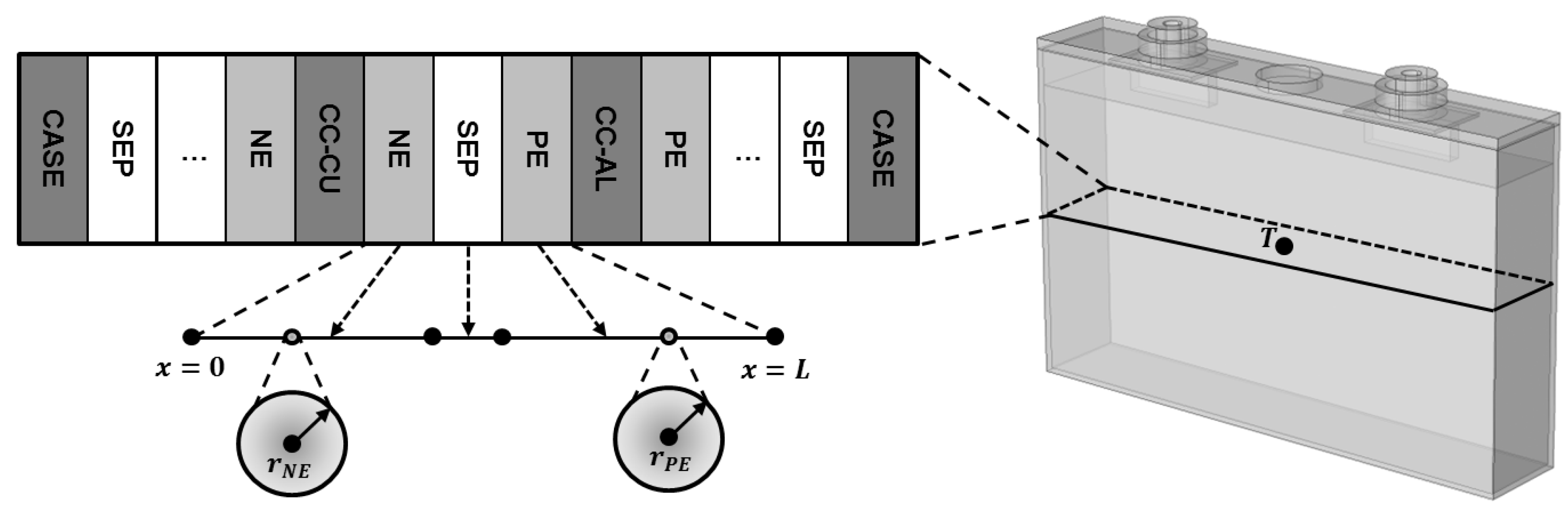
Figure 2.
SEM images of (a) the negative electrode and (b) the positive electrode.
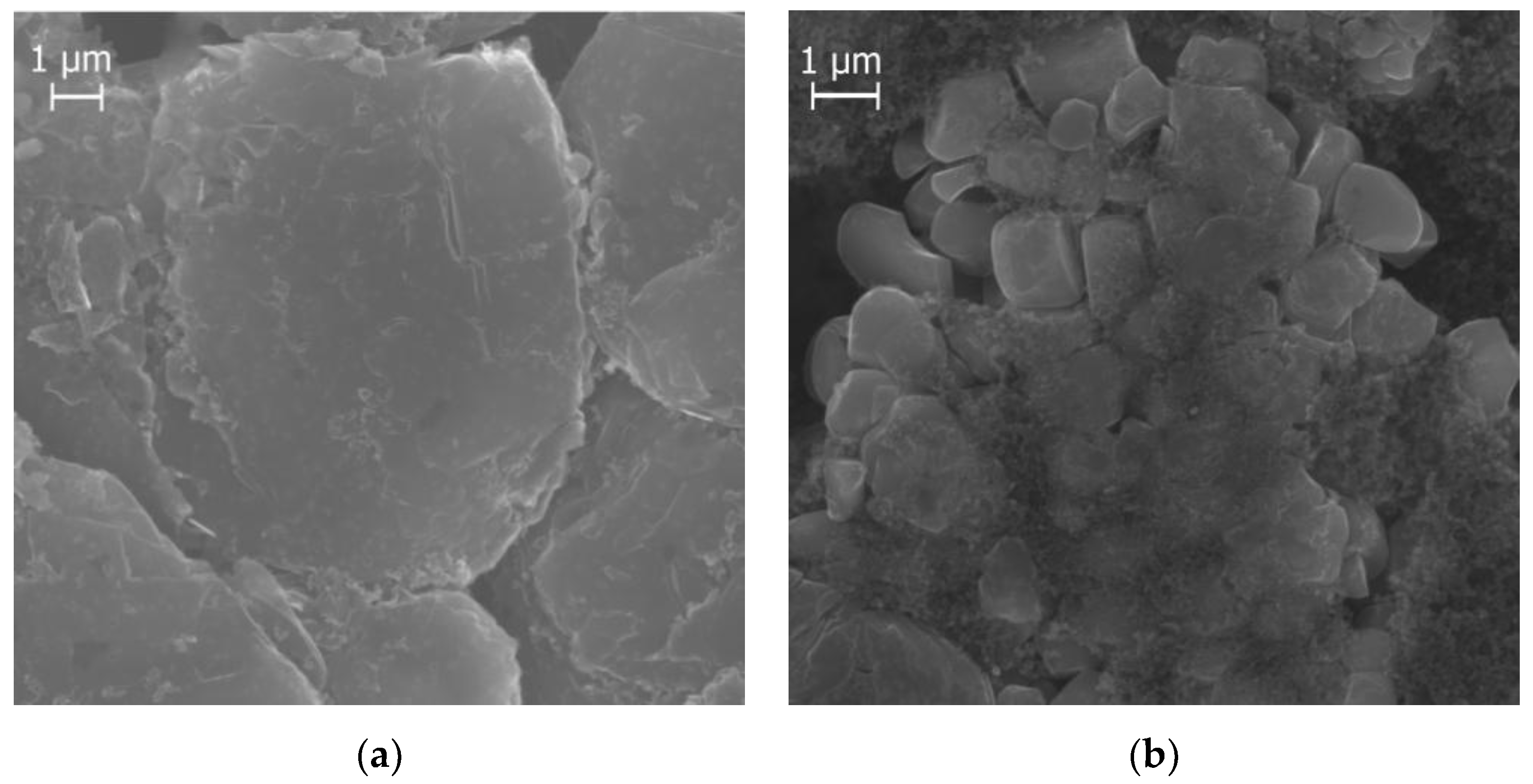
Figure 3.
Experimental and simulated OCV and qOCV profiles (V) as a function of cell SoC and OCV profiles (V) as a function of electrode SoC and intercalation stages at the negative electrode profile.
Figure 3.
Experimental and simulated OCV and qOCV profiles (V) as a function of cell SoC and OCV profiles (V) as a function of electrode SoC and intercalation stages at the negative electrode profile.

Figure 4.
Experimental vs. fitting results of the cell impedance model: (a) Nyquist plot (b) Contribution of real impedance (mΩ) and (c) negative imaginary impedance (mΩ) as function of frequency (Hz).
Figure 4.
Experimental vs. fitting results of the cell impedance model: (a) Nyquist plot (b) Contribution of real impedance (mΩ) and (c) negative imaginary impedance (mΩ) as function of frequency (Hz).
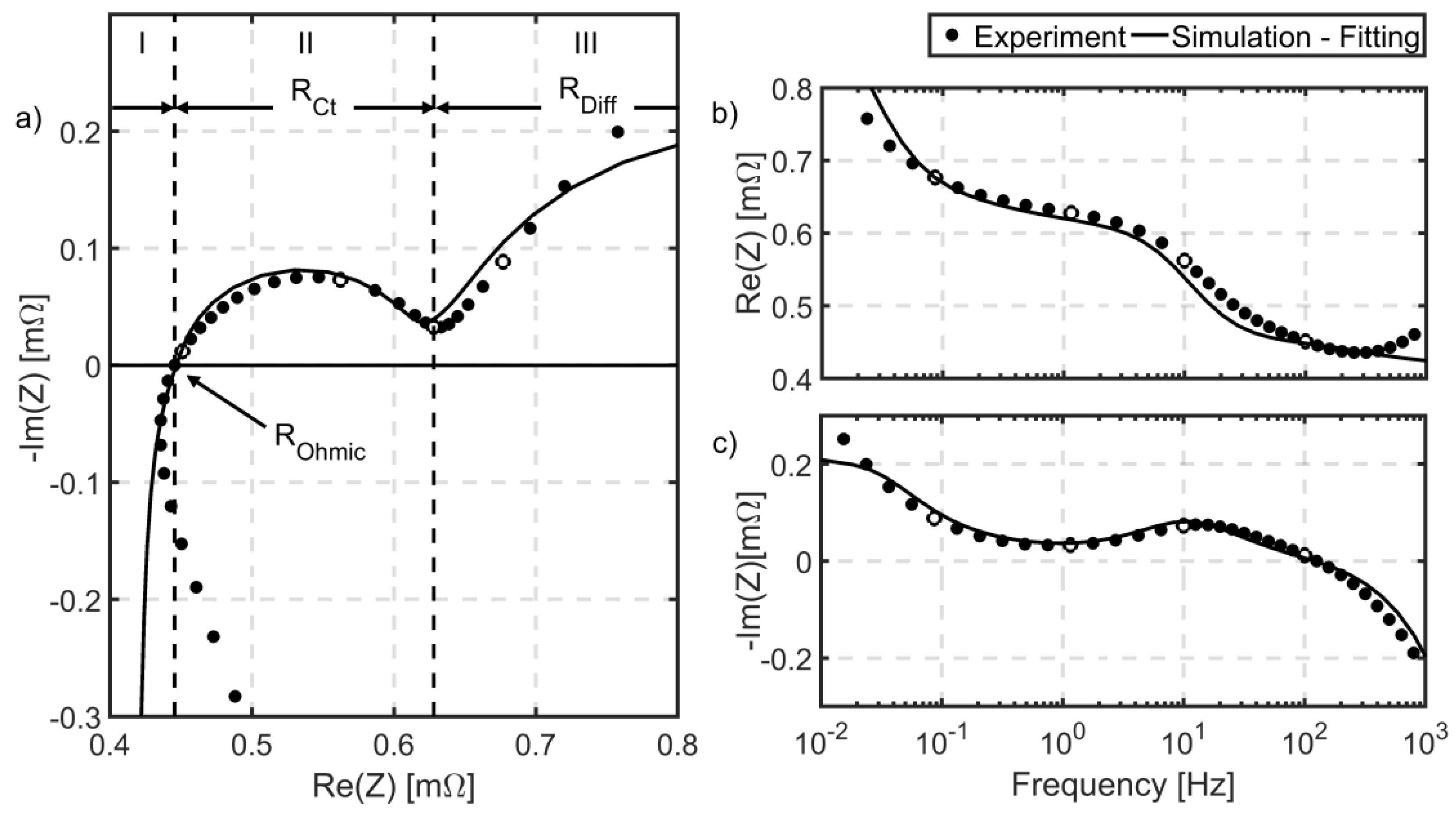
Figure 5.
Experimental and simulated direct current resistance profiles R (mΩ) as a function of cell SoC at the times t = 2 s (a), 10 s (b), 18 s (c) after discharge initialization and t = 10 s (d) after charge initialization.
Figure 5.
Experimental and simulated direct current resistance profiles R (mΩ) as a function of cell SoC at the times t = 2 s (a), 10 s (b), 18 s (c) after discharge initialization and t = 10 s (d) after charge initialization.

Figure 6.
Experimental and simulated cell voltage profile () of the cell as a function of time (s) during a discharge and charge phase at: (a,b) 0.5 C, (c,d) 1 C, and (e,f) 2 C current rates. The cells were initially kept at a constant temperature of 25 °C for multiple hours in a fully charged/fully discharged state.

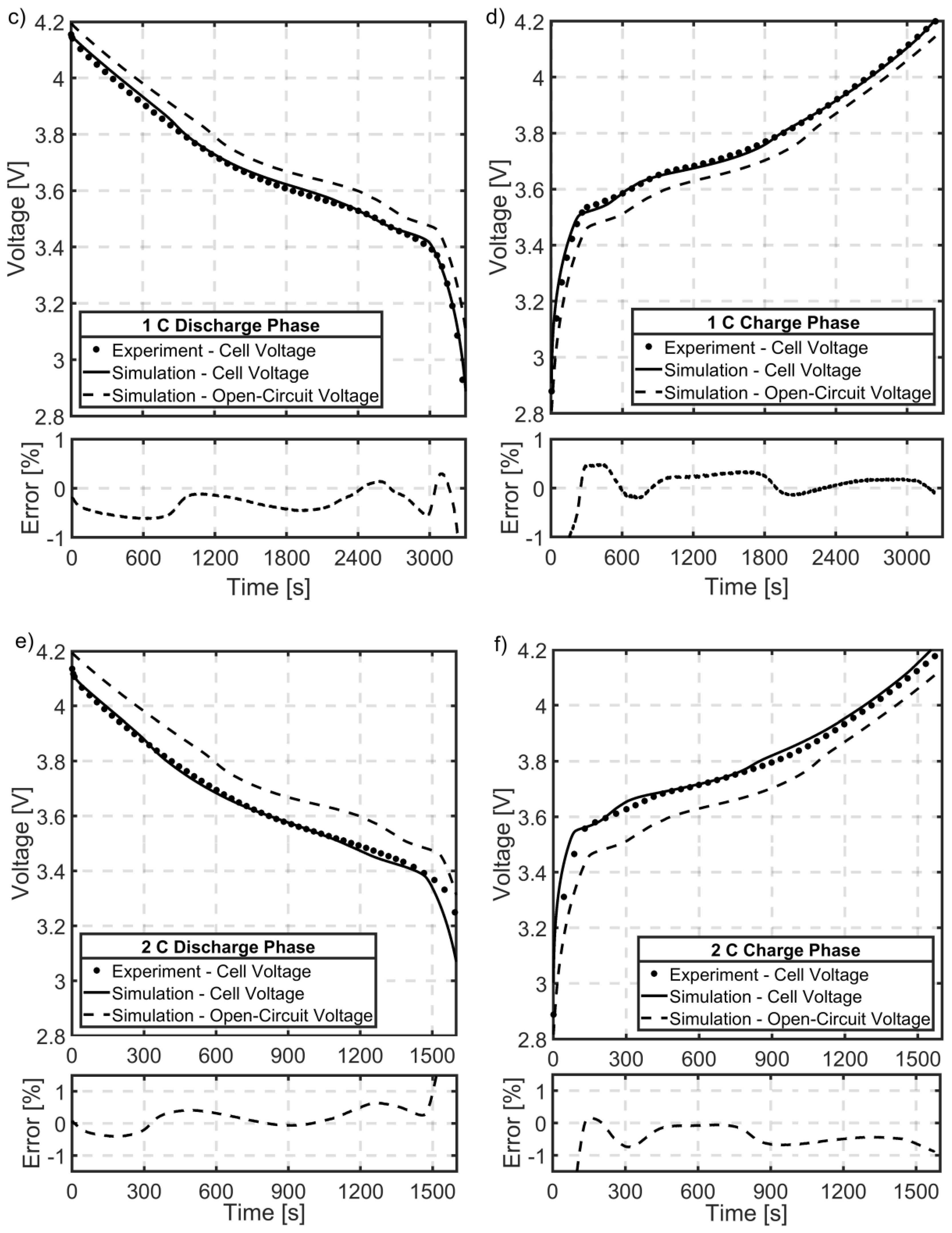
Figure 7.
Experimental and simulated cell temperature profiles () of the cell as a function of time (s) during a discharge and charge phase at: (a,b) 0.5 C, (c,d) 1 C, and (e,f) 2 C current rates. The cells were initially kept at a constant temperature of 25 °C for multiple hours in a fully charged/fully discharged state.
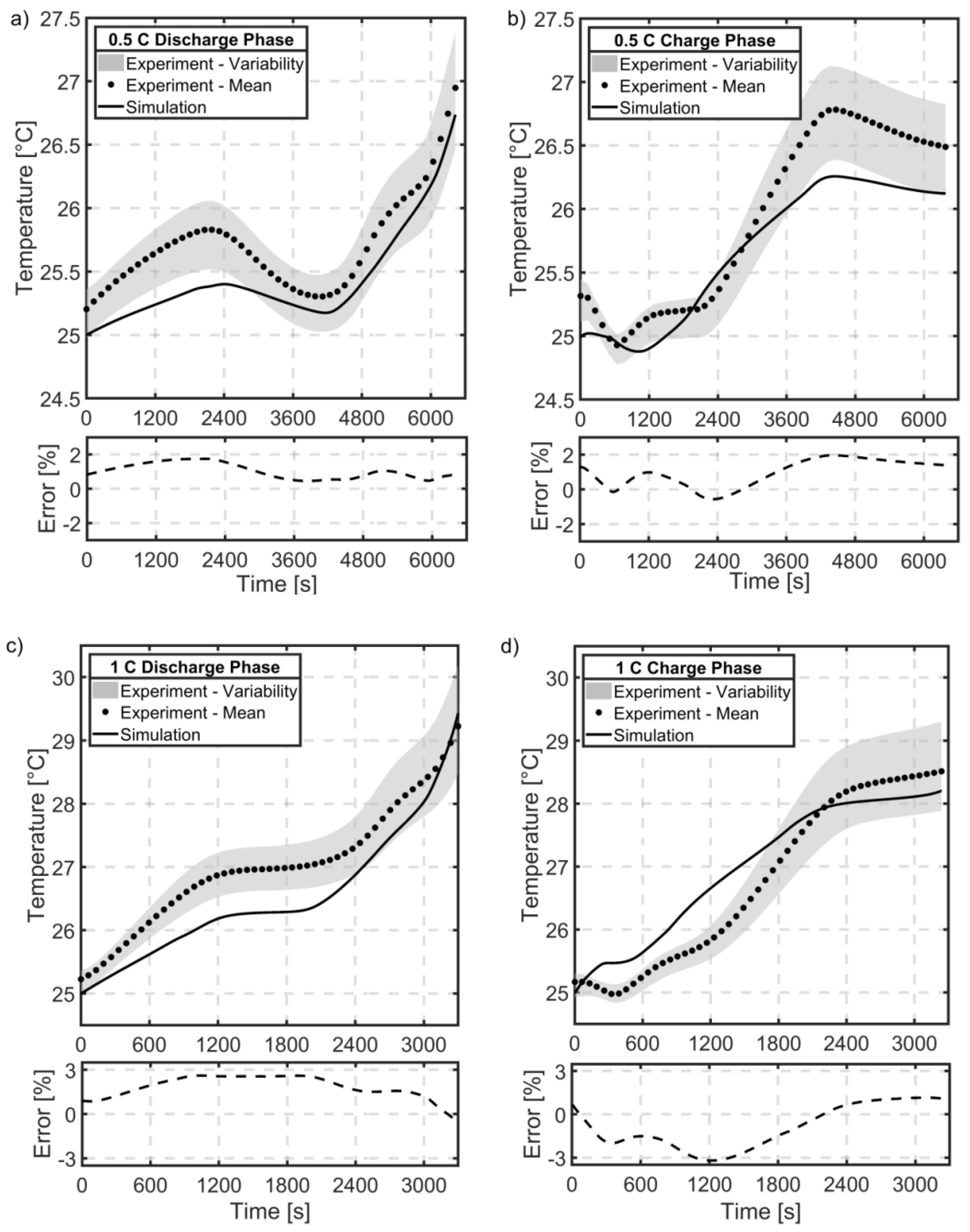

Figure 8.
Simulated heat dissipation density profiles (kW/m3) of the cell as a function of cell SoC (%) during a discharge and charge phase at: (a,b) 0.5 C, (c,d) 1 C, and (e,f) 2 C current rates. The simulated cell temperature profile () is shown for comparison in each case.
Figure 8.
Simulated heat dissipation density profiles (kW/m3) of the cell as a function of cell SoC (%) during a discharge and charge phase at: (a,b) 0.5 C, (c,d) 1 C, and (e,f) 2 C current rates. The simulated cell temperature profile () is shown for comparison in each case.
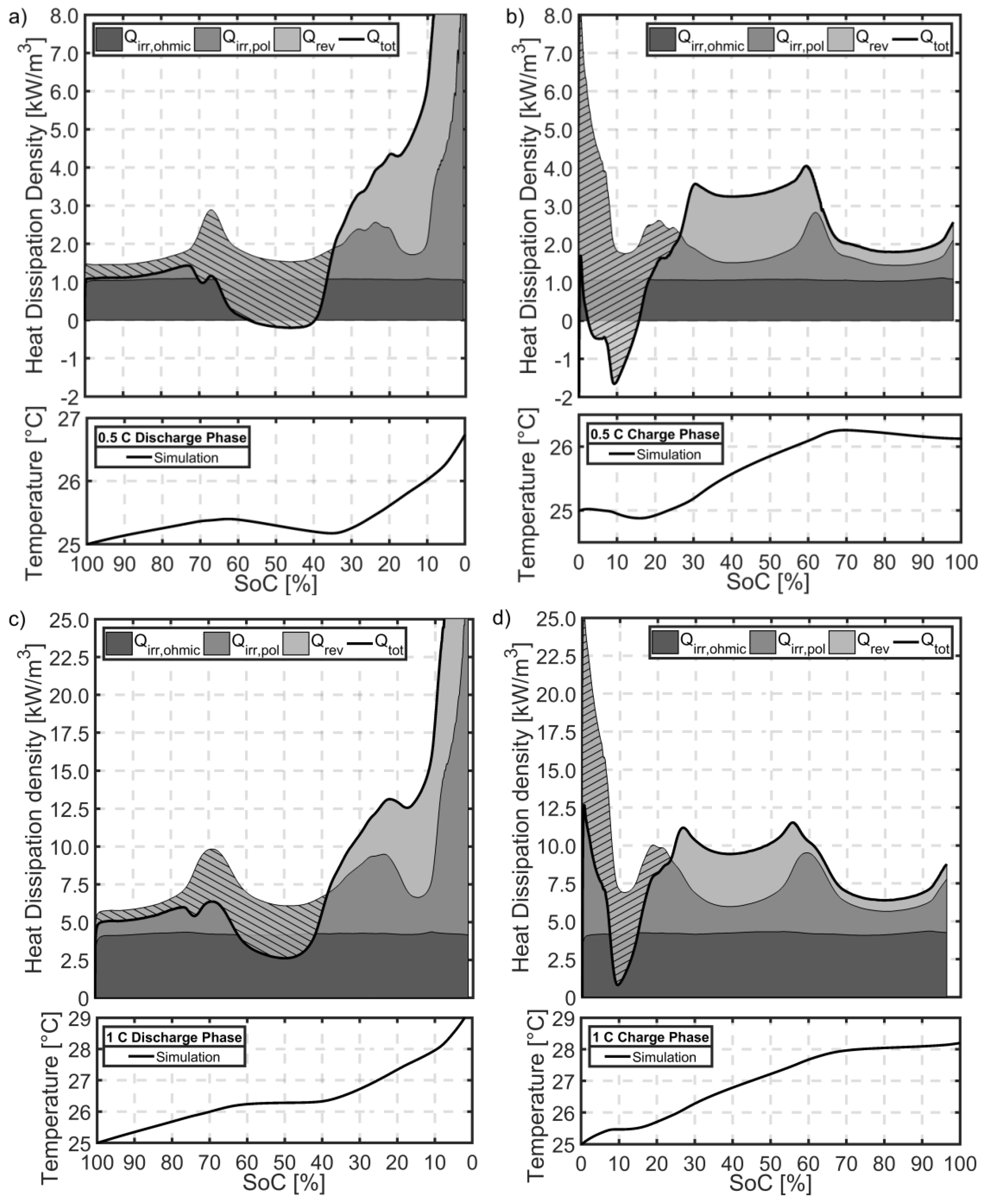
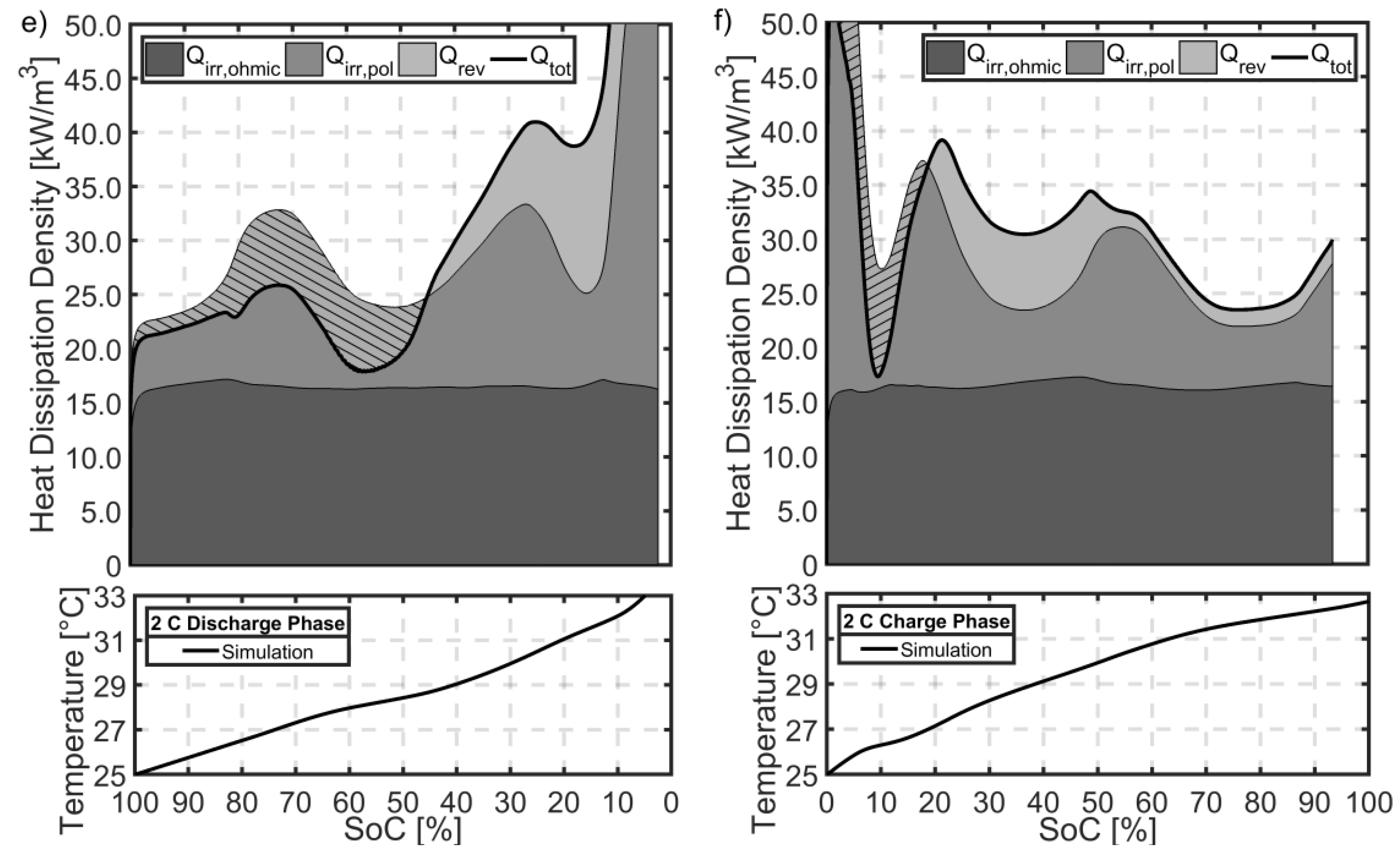
Table 1.
The governing equations of the physico-chemical model.
| Domain/Meaning | Governing Equation | Boundary Condition |
|---|---|---|
| Solid Phase/Electrodes | ||
| Mass Conservation | ||
| Charge Conservation | ||
| Liquid-Phase/Electrolyte | ||
| Mass Conservation | ||
| Charge Conservation | ||
| Reaction Kinetics | ||
| Reaction Rate Pore Wall Flux | ||
| Over-Potential | ||
| Battery | ||
| Terminal Voltage | ||
Table 2.
The heat dissipation sources within the physico-chemical model.
| Domain/Meaning | Equation |
|---|---|
| Electrode | |
| Reversible Heat | |
| Irreversible Polarization Heat | |
| Irreversible Ohmic Heat | |
| Separator | |
| Irreversible Ohmic Heat | |
| Terminal/Current Collector | |
| Irreversible Ohmic Heat | |
| Battery | |
| Total Heat Dissipation | |
Table 3.
Geometrical data of the 40 Ah battery cell.
| Parameter | Symbol | Unit | Anode | Separator | Cathode |
|---|---|---|---|---|---|
| Number of electrode sheets | # | (pc.) | 91 | 90 | |
| Total thickness of one sheet *1 | (µm) | 110.0 | 24.0 | 129.0 | |
| Height for one electrode sheet | (cm) | 8.0 | 8.0 | 8.0 | |
| Width for one electrode sheet | (cm) | 14.6 | 14.6 | ||
| Electrode surface area | (cm2) | 21,258 | 21,024 *2 | ||
| Thickness of current collector *2 | (µm) | 19.01 ± 0.12 *3 | 17.78 ± 1.20 *3 | ||
| Coating thickness | (µm) | 47.5 | 24.7 | 54.5 | |
| Particle Size | (µm) | 9.89 ± 3.31 *3 | 1.72 ± 0.54 *4 | ||
| Porosity | (%) | 30.79 *3 | 19.73 *4 |
*1 measured with µm-screw; *2 , active surface area; *3 measured with µ-CT; *4 measured with n-CT.
Table 4.
The parameter list of volumetric thermo-physical properties of the battery cell for the reference temperature 25 °C.
Table 4.
The parameter list of volumetric thermo-physical properties of the battery cell for the reference temperature 25 °C.
| Material | Density ρ (kg·m−3) | Heat Capacity Cp (J·kg−1K−1) | Volume Fraction (%) |
|---|---|---|---|
| Positive Electrode Coating | 4670 [25] | 940 | 29.29 |
| Negative Electrode Coating | 2260 [25] | 1040 | 25.53 |
| Aluminum [1] | 2700 | 900 | 4.03 *1 |
| 0.26 *2 | |||
| Copper [1] | 8700 | 385 | 5.37 *1 |
| 0.26 *2 | |||
| Separator | 1009 | 1907 | 12.9 |
| Steel [52] | 8030 | 502.48 | 13 |
| Synthetic (Acrylic Plastic) [20] | 1190 | 1470 | 9.36 |
*1 inside electrode stack; *2 outside electrode stack.
Table 5.
The parameter list of the surface-related thermo-physical properties.
| Material | Emissivity ϵ | Surface Area (cm2) |
|---|---|---|
| Isolating Tape | 0.97 | 399.20 |
| Steel | 0.74 | 11.11 |
| Synthetic (Acrylic Plastic) | 0.95 | 0.695 |
Table 6.
Summary of all the material and cell properties resembling the analyzed battery cell.
| Definition | Symbol | Unit | Negative Electrode | Separator | Positive Electrode | Reference |
|---|---|---|---|---|---|---|
| Design Specifications | ||||||
| Domain Thickness | L | (µm) | 47.5 | 24.7 | 54.5 | Table 3 |
| Electrode Plate Area | A | (m2) | 2.1024 | Table 3 | ||
| Particle Radius | (µm) | 9.89 | 1.72 | Table 3 | ||
| Actual Capacity | (Ah) | 48.17 | 69.20 | Equation (10) | ||
| Active Electrode Volume | (cm3) | 99.86 | 114.58 | |||
| Molar Mass | (g/mol) | 72.0 | 96.5 | [25] | ||
| Density | (kg/m3) | 2260 [61] | 4670 [62] | [25] | ||
| Theoretical Capacity | (Ah) | 84.01 | 148.61 | Equation (11) | ||
| Lower Electrode SoC | 0.01 | 0.415 | Fitted: OCV | |||
| Upper Electrode SoC | 0.785 | 0.955 | Fitted: OCV | |||
| Active Material Fraction | 0.548 | 0.457 | Equation (12) | |||
| Specific Surface Area | (m-1) | 172,730 | 825,880 | Equation (13) | ||
| Surface Area | (m2) | 17.25 | 94.63 | Equation (14) | ||
| Electrolyte Volume Fraction | 0.308 | 0.395 [25] | 0.191 | |||
| Inactive Volume Fraction | 0.189 | 0.45 | Equation (9) | |||
| Kinetic and transport properties | ||||||
| Open-Circuit Potential | U | (V) | Equation (6) | Equation (5) | Fitted OCV, [25] | |
| Temperature derivative of Open-Circuit Potential | (V/K) | Taken from [32] | [63] | [32,63] | ||
| Charge Transfer Symmetry Factor | 0.5 | 0.5 | [36] | |||
| Maximum Lithium Intercalation Concentration | (mol/m3) | 31,389 | 48396 | [25] | ||
| Equilibrium Electrolyte Concentration | (mol/m3) | 1000 | 1000 | 1000 | [25] | |
| Effective Electrode Diffusion Coefficient | (m2/s) | Equation (25)/(26) | Equation (25)/(27) | [25] | ||
| Reference Electrode Diffusion Coefficient | (m2/s) | Equation (26) | Equation (27) | [25] | ||
| Effective Electrode Electronic Conductivity | (s/m) | Equation (34) | Equation (34) | [25] | ||
| Reference Electrode Electronic Conductivity | (s/m) | 100 | 10 | [25] | ||
| Effective Electrolyte Conductivity | (s/m) | Equation (32) | [50] | |||
| Reference Electrolyte Conductivity | (s/m) | Equation (33) | [50] | |||
| Bruggeman Exponent | 1.5 | 1.5 | 1.5 | [3] | ||
| Effective Diffusional Electrolyte conductivity | (s/m) | Equation (35) | [52] | |||
| Effective Electrolyte Diffusion Coefficient | (m2/s) | Equation (28) | [50,51] | |||
| Reference Electrolyte Diffusion Coefficient | (m2/s) | Equation (29) | [50] | |||
| Li-transference Number | Equation (30) | [50] | ||||
| Effective Electrolyte Activity coefficient | Equation (31) | [50,51] | ||||
| Reaction Rate Coefficient | (m2.5/mol0.5s) | Fitted: EIS | ||||
| Double Layer Capacitance | (F/m2) | 5.18 | 0.96 | Fitted: EIS | ||
| Ohmic Resistance | (mΩ) | 1.24 | Fitted: EIS | |||
| Inductance | (H) | Fitted: EIS | ||||
| Exchange Current Density Activation Energy | (kJ/mol) | 48.9 | 78.1 | [25] | ||
| Electrode Diffusion Activation Energy | (kJ/mol) | 28.8 | 49.6 | [25] | ||
| Electrolyte Diffusion Activation Energy | (kJ/mol) | 16.5 | [51] | |||
| Electrolyte Conductivity Activation Energy | (kJ/mol) | 4.0 | [51] | |||
| Electrolyte Activity Coefficient Activation Energy | (kJ/mol) | −1.0 | [51] | |||
| Thermal parameters | ||||||
| Heat Capacity | (J/kgK) | 1055.1 | Equation (37) | |||
| Density | (kg/m3) | 3179.66 | Equation (36) | |||
| Battery Volume | (cm3) | 371.08 | Measured | |||
| Electrode Stack Volume | (cm3) | 286.16 | Measured | |||
| Convective Heat-Transfer Coefficient | (W/m2K) | 6.9 | [36] | |||
| Convective Cooling Surface Area | (cm2) | 415.99 | Measured | |||
| Area-specific Emissivity | (cm2) | 402.05 | Equation (38) | |||
© 2019 by the authors. Licensee MDPI, Basel, Switzerland. This article is an open access article distributed under the terms and conditions of the Creative Commons Attribution (CC BY) license (http://creativecommons.org/licenses/by/4.0/).
Share and Cite
MDPI and ACS Style
Liebig, G.; Gupta, G.; Kirstein, U.; Schuldt, F.; Agert, C. Parameterization and Validation of an Electrochemical Thermal Model of a Lithium-Ion Battery. Batteries 2019, 5, 62. https://doi.org/10.3390/batteries5030062
AMA Style
Liebig G, Gupta G, Kirstein U, Schuldt F, Agert C. Parameterization and Validation of an Electrochemical Thermal Model of a Lithium-Ion Battery. Batteries. 2019; 5(3):62. https://doi.org/10.3390/batteries5030062
Chicago/Turabian StyleLiebig, Gerd, Gaurav Gupta, Ulf Kirstein, Frank Schuldt, and Carsten Agert. 2019. "Parameterization and Validation of an Electrochemical Thermal Model of a Lithium-Ion Battery" Batteries 5, no. 3: 62. https://doi.org/10.3390/batteries5030062
Note that from the first issue of 2016, this journal uses article numbers instead of page numbers. See further details here.