A Suggested Improvement for Small Autonomous Energy System Reliability by Reducing Heat and Excess Charges


1
Mainate Labs, 77430, 25 rue de Sens, Champagne-sur-Seine, 77430, France & GEII Department, IUT Gratte-Ciel, 17 rue de France, 69627 Villeurbanne Cedex, France
2
Electromechanical Department, Saint-Petersburg Mining University, 21st line 2, Saint-Petersburg 199106, Russia
*
Author to whom correspondence should be addressed.
Batteries 2019, 5(1), 29; https://doi.org/10.3390/batteries5010029
Submission received: 30 January 2019
/
Revised: 19 February 2019
/
Accepted: 6 March 2019
/
Published: 11 March 2019
(This article belongs to the Special Issue Batteries and Supercapacitors Aging)
Abstract
:Devices operating in complete energy autonomy are multiplying: small fixed signaling applications or sensors often operating in a network. To ensure operation for a substantial period, for applications with difficult physical access, a means of storing electrical energy must be included in the system. The battery remains the most deployed solution. Lead-acid batteries still have a significant share of this market due to the maturity of their technology. However, even by sizing all the system elements according to the needs and the available renewable energy, some failure occurs. The battery is the weak element. It can be quickly discharged when the renewable energy source is no longer present for a while. It can also be overloaded or subjected to high temperatures, which affects its longevity. This paper presents a suggested improvement for these systems, systematically adding extra devices to reduce excess charges and heat and allowing the battery use at lower charges. The interest of this strategy is presented by comparing the number of days of system failure and the consequences for battery aging. To demonstrate the interest of the proposed improvement track, a colored Petri net is deployed to model the battery degradation parameters evolution, in order to compare them.
1. Context
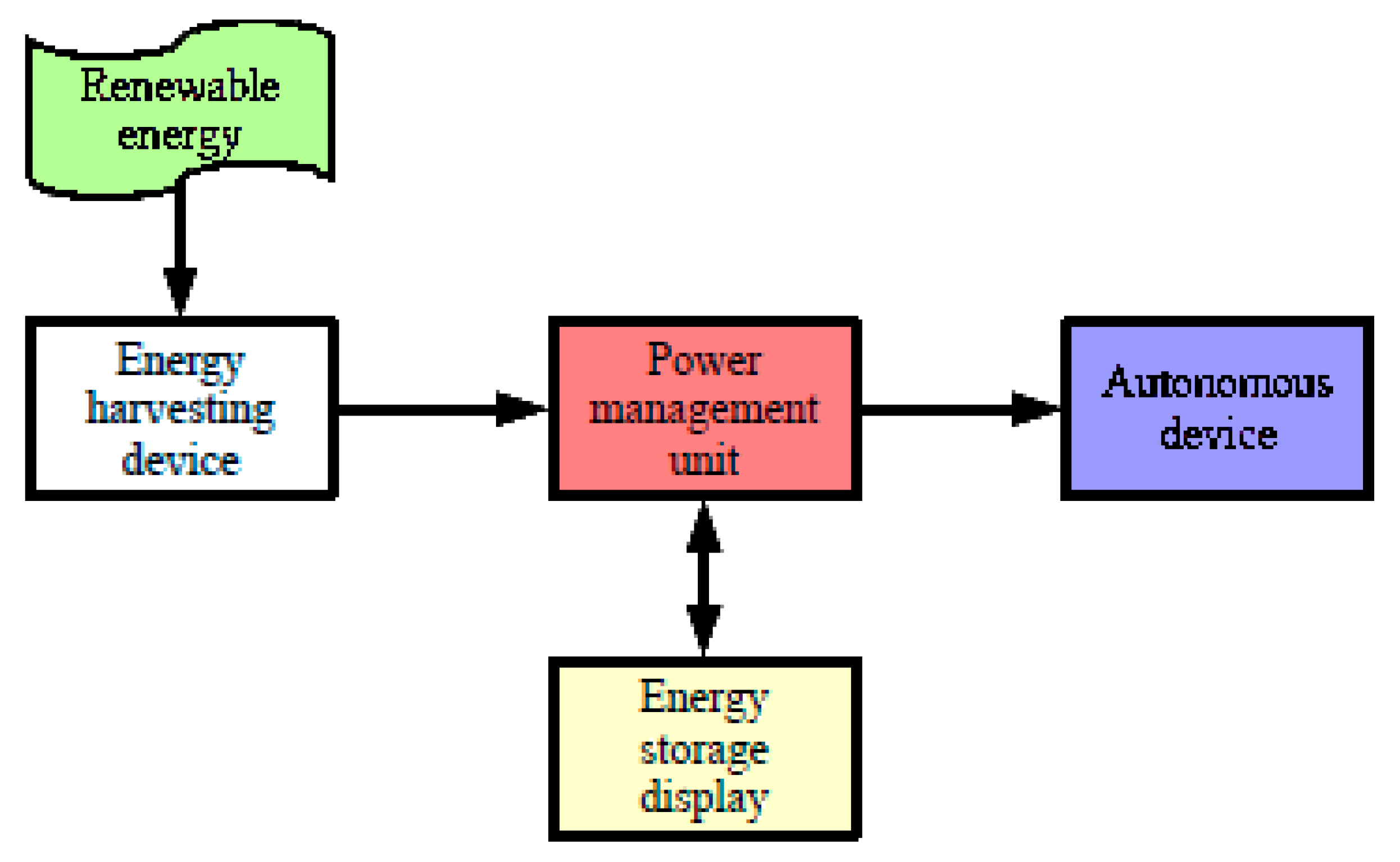
Some devices operate autonomously by drawing and harvesting available energy in their environment. These kinds of devices are often used for signaling or for compilation and information data storage [1]. In this case, the sensors can have a network connection. Having an opportunity to provide renewable energy provides these small applications with sustainability in the achievement of their mission, which is not always the case for networks of sensors located in inaccessible places and subject to strong constraints that thus must optimize their consumption and their communications [2]. This paper looks at devices profiting daylight, but for which systematic forecast maintenance visits are spaced out over time. These stand-alone systems are often designed according to the schematic diagram in Figure 1. This is the case for devices that collect solar energy and convert it into electrical energy to power a device that operates continuously [3,4]. To take into account the weather conditions of the implantation site, it is necessary to associate a source of electrical energy storage [5]. For this, one or more batteries are included in the system. These batteries are often still lead-acid batteries because their mature technology, proven for many decades; their high mass and volume capacity, still superior to the present Li-ion batteries [6,7]; their apparent robustness; and their low production cost relative to the stored kilowatt-hour, make them competitive. They retain a significant market share, particularly since they can operate under low temperatures. This is especially true since it is necessary to oversize the battery in order to operate in the most degraded conditions: in winter, in rainy weather, or when the energy sensors are hidden under accumulated snow. Right now, however, power management units (PMUs), even though they are responsible for energy security and optimization, are not functioning optimally. Thus, the battery is often overcharged in summer, which causes rapid aging, shortening the system’s useful operating time before failure. The failure consists of a current providing termination to the autonomous device. It is possible to add a complementary energy storage system to the autonomous device, for example, with a flywheel or in the form of thermal storage [8]. This avoids short feeding breaks, but is not enough in winter. Indeed, the low level of brightness associated with short periods of sunshine can also lead to battery discharges, such as the PMU disconnecting the autonomous device to protect the battery by discharging too much. The periods of low light are often long in winter and a second remote energy storage system should then be sized taking into account the probable duration of power failure. As a matter of principle, the PMU only works in two modes: Safe and Functional. A good quality PMU monitors the battery voltage to switch modes and also to set the battery charge mode, sending power from the energy harvesting system (EHS) when it is surplus to the device requirements, respecting as much as possible the principle of a charge in continuous current (CC) mode followed by a continuous voltage (CV) mode when the charge is close to its maximum. However, this does not guarantee that the battery lifespan is optimized. This paper proposes a simple approach to modeling battery aging and uses a Petri net to simulate the influence of the proposed adaptations on the aging aggravation. It suggests improvement to optimize energy management and reduce premature aging, even if it sometimes means current-shedding the device.
2. Battery Aging Issue
Lead-acid batteries used in these systems consist of several cells connected in series to provide the required voltage. The degradation of performance that results from aging cells is the consequence of three main phenomena, which are related to each other [9]. In the first place, the electrodes corrode, mainly during excessive recharges and when the battery remains in full charge for a long time. The positive electrode loses some of the active mass at each recharge-discharge cycle, but not linearly and continuously throughout the electrode. This reduction in mass decreases the amount of electrical charge that can be stored in the battery. In the second place, the electrodes cover themselves with lead sulphate. This sulphation is mainly related to a high depth of discharge (DoD) [9]. Typically, when the battery contains less than 25% of its maximum charge, it is considered in deep discharge. PMU manufacturers consider that SoC = 25% is a threshold below which the battery should not be discharged. Actually, below this threshold, the OCV decline accelerates because under low charges, the electrolyte contains only a low acid concentration. During a discharge, it is strongly diluted in the electrolyte [10]. The larger the DoD, the lower the acid concentration. In the third place, the amount of electrolyte decreases with use. This is the phenomenon of drying out, following the evaporation of water appearing during the chemical reactions [11]. This can be a result of high charges or high ambient temperature.
Obviously, even occasional battery short-circuiting aggravates its degradation. The PMU makes sure to remove this risk. A battery in deep discharge can be permanently damaged by sulphation. If the sulphate of lead formed during a weak discharge has a very fine crystalline structure, which will be easily decomposed by the charging current, the lead sulphate crystals created during the deep discharges are too big to be dissolved by the charging current [12]. In addition, the larger the crystals, the faster the voltage between the electrodes increases during recharge and decreases during discharge, reducing the amount of energy stored and restored [10]. When a battery remains discharged for too long, the lead particles dissolve in the electrolyte, and the solubility increases. They then form a lead hydrate, which crystallizes in the separator [9]. If these crystals come into electrical contact, pure lead dendrites (growth in branching) form and grow progressively, increasing self-discharge. This hydration phenomenon leads to internal short circuits. To reduce the formation of crystals, it is possible to resort to the pulsed-current technique [13,14] during fast refills and thus to reduce the effects on the aging aggravation. The pulse-current charging strategy is employed to recharge the battery with a direct current to which a middle frequency alternating current is added. This pulsed-current technique increases the battery lifespan [14] because it reduces the amount of lead crystals in the active material and minimizes the development of lead hydrate [12,13]. Corrosion also occurs due to self-discharge reactions between the lead and the sulfuric acid of the electrolyte. Under normal charging conditions, a protective layer of lead oxide is formed. It is unfortunately dissolved if the battery is discharged and the acid concentration is low, causing an acceleration of corrosion. Corrosion is irreversible.
The PMU measures the voltage across the battery [15]. It uses an internal model based on the relation that exists between the electric charge Q(t) contained in the battery and the terminal voltage Vbat, even if it is not identical for the same charge, depending on whether the battery is recharging or discharging. Depending on Vbat, the system is placed in one of two operational modes. Any type of model allows the battery lifespan to be determined after calculation provided that it is based on a sufficient quantity of parameters and that it includes a suitable description of aging processes [11]. However, since Sauer and Al. [16] recall that no model perfectly correlates the aging processes of lead-acid batteries and their impact on performance, it is superfluous to resort to a perfectly precise model.
One of the advanced-PMU missions is to limit conditions that will accelerate degradation, such as maintaining a small size for sulphate crystals to avoid deep discharges, operating at a not too high ambient temperature to reduce internal evaporation, or finally reducing the time during which the battery is fully charged (cause of accelerated corrosion). In a contradictory manner, in order to limit the sulphation, it is necessary to regularly carry out a complete recharge, typically under a temperature oscillating around 45 °C, at least once every month. On the other hand, when the cell voltage falls below 2.1 V, the corrosion already present accelerates. Optimally, a cell voltage close to 2.25 V, called the float voltage, reduces corrosion. This voltage is often recommended in power supply systems for which corrosion is a major factor in aging. For a classic 12 V battery, consisting of six cells with a nominal voltage of 2.1 V, this leads to an ideal float voltage of 13.5 V. In applications such as autonomous photovoltaic panel power systems (A3PS), the battery continually discharges in the absence of sun, even when it does not provide power, due to its self-discharge. Typically, this self-discharge is close to 10% per month.
The battery conditions of use contribute to its aging and the acceleration of it. Cycling is another phenomenon that reduces the battery lifespan used in an A3SP. Since charge regularly oscillates between a maximum (often the full charge) and a minimum (close to the deep discharge), it combines the corrosion and its aggravation. In addition, the batteries must not be placed on undercharging for long periods of time, otherwise sulphation will occur. The temperature has a positive influence on the battery capacity, which increases by just under 1% per degree Celsius. Since sulphate crystals are more readily dissolved at an elevated temperature, it appears preferable to perform regular full charges at a high temperature while keeping the battery at a lower temperature outside these times.
This paper is organized as follows: after recalling the different causes of lead-acid batteries aging, a simple cell model based on different parameters is proposed in order to control the aging. To achieve this, Part IV will present an implantable model in the PMU to track battery operation, as well as a suggested improvement track. The model is based on Petri nets, whose principles are recalled in the previous chapter. Finally an example of A3SP is presented before its operation is analyzed by comparing the impact on aging of the suggested improvement.
3. Battery Parameters
In a conventional approach, the battery can be modeled as a voltage generator according to the first or second order model of Thevenin. The open circuit voltage (OCV) is related to the amount of electric charge in the battery at time t, denoted Q(t). The battery can store a maximum amount of charge, noted as Q0, which will decrease with aging, so with time t. Therefore, to quantify the charge contained in the battery, it is defined as a state of charge (SoC) at any time t, defined by Equation (1).
The equivalent series resistance (ESR) of the first order Thevenin model reflects the electrical consequences of heat loss in the electrolyte and in the connections, as well as the ohmic resistance of the electrodes and connections. The resistance value grows with aging since it represents a brake on the current flow in the physical structure of the battery.
Aging is directly related to the battery use: cycling, charges and deep discharges, operating, and storage temperature. In cells, the lead (Pb) and lead oxide (PbO2) conversion to PbSO4 during the reaction with electrolyte sulfuric acid induce high mechanical stress, and the volumes of PbSO4 are about double. The weak charge fluctuation only leads to small variations in the electrolyte volume and thus to lower mechanical stresses that will have less impact on cell aging. Deep discharges cause corrosion and sulphation. We consider that a battery that operates under optimal conditions must age in the same way as when it was tested and that its lifespan was determined by its manufacturer. Optimally, the charge varies around a float capacity at each cycle. The float voltage which ensures the least possible aging for a battery, also when it is not stressed [17], is thus close to 2.25 V. This value corresponds to SoC = 0.85. Subject to different operating regimes, its aging will worsen. Thus, beyond a charge fluctuation of 30%, the impact on aging can be considered to increase linearly. On the other hand, to model the temperature impact, it is possible to use the Arrhenius law, because of the electrochemical reaction process temperature dependence. In a simplified manner, it is generally considered that the service life is halved for a device operating at a temperature of 10 °C and above. For a lead-acid battery, the optimum operating temperature is close to 30 °C, as specified by Gauri and Al [18].
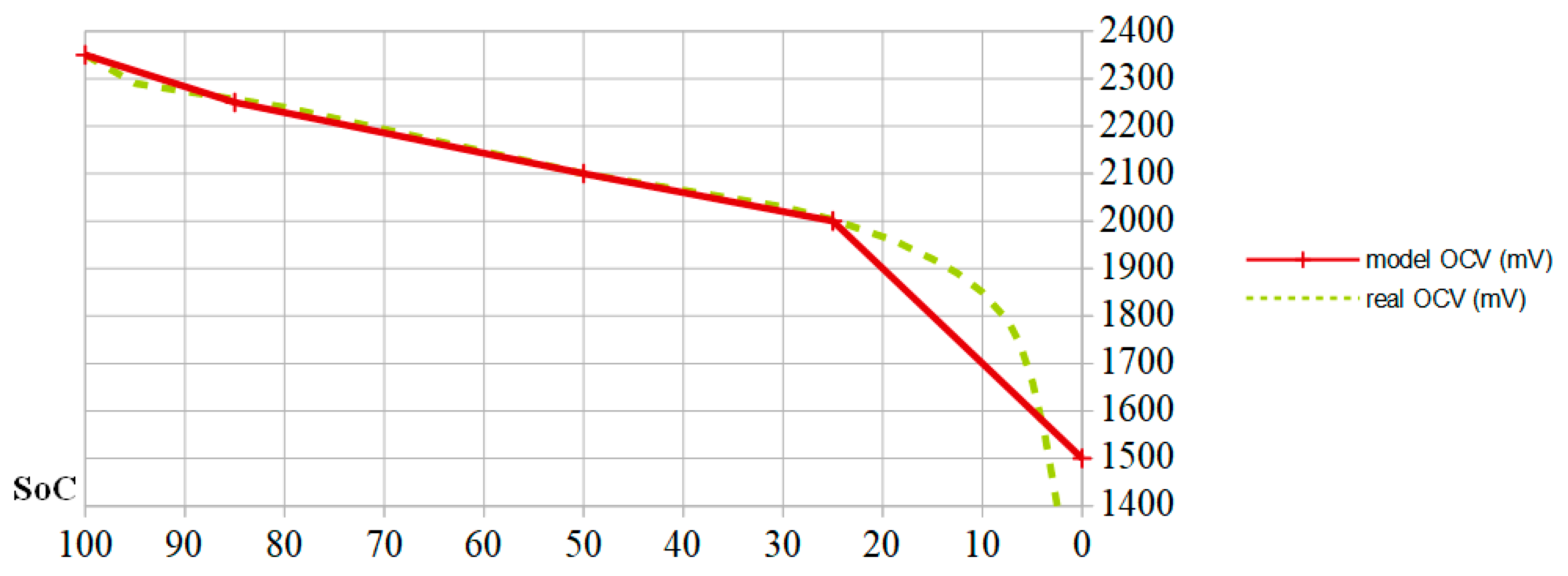
Some articles, such as [19], are based on a neural network to model a lead-acid battery operation and integrate aging, so as to overcome the parameter variability through self-learning and model parameter correction. Indeed, the estimate lead-acid battery SoC is more delicate than for more modern technologies because many side reactions occur in the electrolyte and interfaces, in addition to the losses incurred during the charging process. Haddad and Al. propose a model differentiating the series resistance according to the current direction, in parallel with an over-voltage capacity simulating the return to the thermodynamic equilibrium after a recharge or a discharge. The cell voltage is different, depending on whether it is recharging (higher voltage) or discharging (lower voltage), because of relaxation phenomena [20]. A voltage generator controlled by the SoC is completed in parallel by a resistor representing the self-discharge. In [21], the SoC calculation precision is dependent on the number of equations, allowing the authors to integrate the variable parameters such as the temperature, the quantity of electrolyte, and the electrode sizes, as well as the aging. However, in a PMU, the SoC is often determined from the simple OCV measurement, with corrective measures made when the battery is placed at rest or following heuristic methods. The present work does not retain the principle of system operation real-time monitoring, but focuses on the state in which it is at dusk. If during the daytime, the autonomous device has not been fed continuously, it is considered that the system has failed. Thus, the parameters to be followed for the battery are the SoC and the OCV voltage, and for the system, the parameter is if the mission has been fulfilled or not. Finally, based on the operating conditions influencing the battery lifespan, we define a fourth parameter: aging aggravation, noted as Agg. If the battery operated under optimum conditions (temperature close to 30 °C, average OCV close to the 2.25 V float voltage, and daily charge variation less than 30%), Agg would be worth 1. Reference [22] shows that the battery lifespan can be considerably reduced when it does not work under these conditions. We will then consider that the following three phenomena, when in convolution, lead to aggravation Agg = 8: high temperature, full charge, and low SoC. In the latter case, we consider two thresholds: a strong degradation threshold for SoCs less than 25% (inducing a factor 2) and average degradation for SoCs less than 50% (inducing a factor of 1.5). This is the reason why the current PMUs shed the autonomous device as soon as the cell OCV falls below 2.1 V, i.e., 12.6 V for a six-cell battery. This voltage corresponds to SoC = 50%, as shown schematically in Figure 2, showing the relation between SoC and OCV as a yellow dotted line, expressed in mV, for a 24 Ah lead-acid battery cell. When the cell is charged at half of its capacity (SoC = 0.5), its OCV reaches the nominal value of 2.1 V. The more the cell is charged, the higher its OCV is. When the cell approaches full charge, its OCV increases faster with SoC. As previously indicated, the OCV decreases more quickly when SoC is less than 25%.
Since the model describing the relationship between electric charge and OCV does not need to enter either the chemical parameters evolution trend or the electrical parameters evolution, but must follow the four previously defined parameters, the fundamental relation between the SoC and the OCV can be simplified according to the red line in Figure 2. This allows the voltage to be expressed with respect to the state of charge according to three linear zones. The limits between these zones correspond to SoC = 0.85 (float capacity), SoC = 0.5 (voltage of 2.1 V serving as a threshold for current PMUs), and SoC = 0.25 (threshold before a deep discharge causing sulphation). Finally, the battery self-discharge must be integrated into the A3PS energy balance.
4. Petri Net Tool
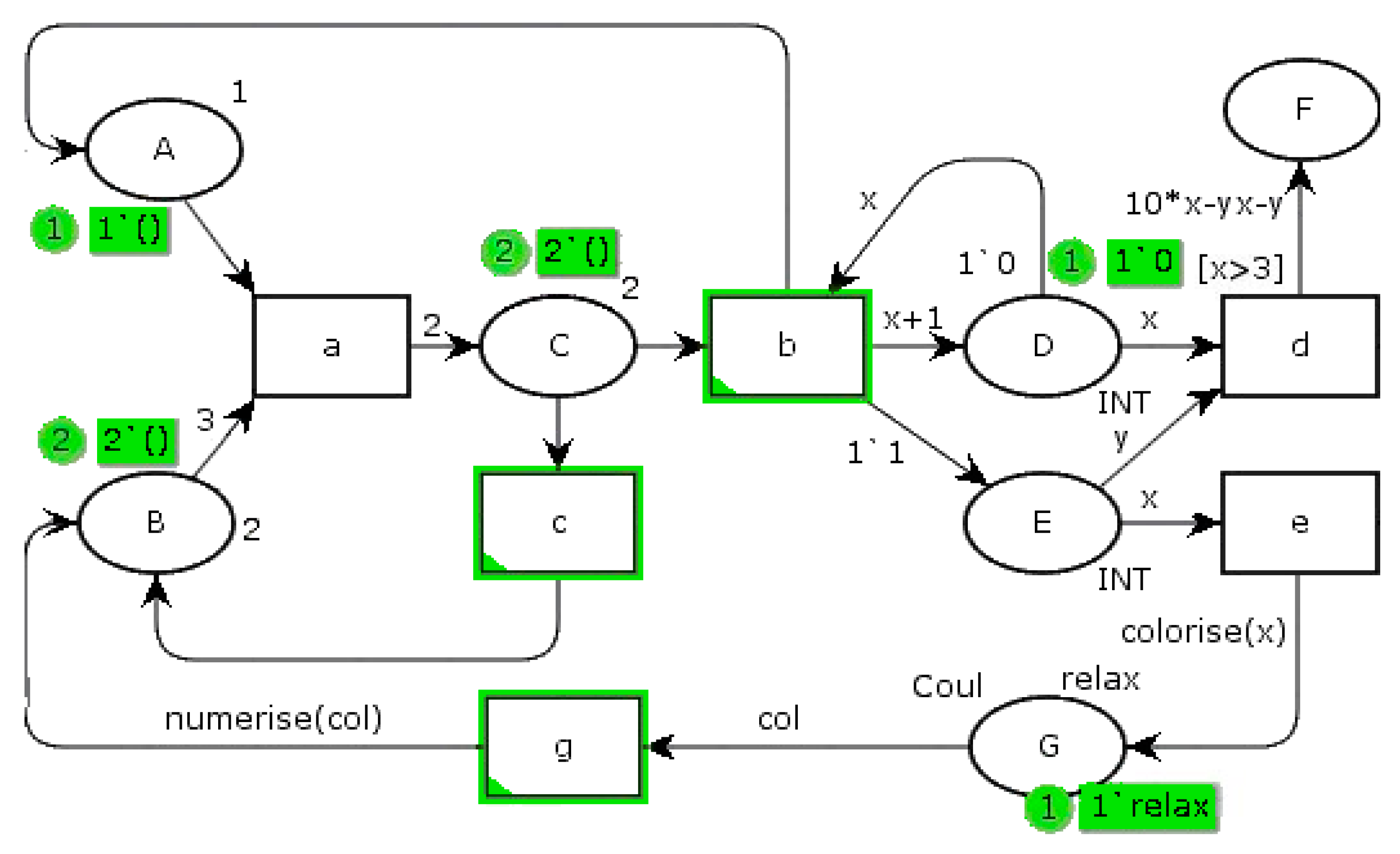
In order to realize simulation of cell behavior and parameters evolution, a Colored Petri network (PN) is proposed [23]. Figure 3 shows an example of a PN, which associates formal semantics and visual representation with precise syntax and a graphical language, unlike a state machine with its own alphabet. A PN is represented by a graph, consisting of states, transitions, and arcs connecting these states and transitions. It belongs to the world of discrete events. An event is embodied by the firing of a transition. The operation of the system described by an PN is thus visualized by a synthetic structured and compact representation. Formally, a PN has properties such as liveliness, boundary, persistence, and reset [24]. Dedicated mathematical tools ensure that it is analyzed.
In a PN, ovoids represent the states, for example, state “A”. Transitions are represented by rectangles, i.e., transition “a”. Oriented arcs link them, implying a consecutive relationship. The states may contain a marking of one or more tokens, as one token in state “A” and two in state “B”. When at least one token is in a state, this state is active. On the contrary, state “F” is not active. When all upstream states are marked (contain at least one token), the transition is firable. If the associated guard is respected, it is shot. A guard is a logical condition on upstream markings and/or on external variables. For instance, “d” transition guard “[x > 3]” means that state “D” has to contain at least three tokens. Arcs can be weighted by a number of needed tokens greater than unity. Then, the net is designated as a generalized Petri net. The upstream place token(s) are then transferred to the downstream state(s). In the Figure 3 example, if a token is present in state “A” and three tokens are in state “B”, transition “a” can be passed. In this case, state “C” acquires two additional tokens. On the other hand, if a token is present in state “E” and state “D” contains at least three tokens, transition “d” is fired. A function weights the arc, leading to state “F”. So, here it receives 10x-xy-y tokens.
Tokens can have different colors. A color assigned to a token may, for example, be a set of positive integers (color INT, for integer); boolean (BOOL); a restriction of some listed elements, such as integers from 0 to 10; or a list of predefined colors, such as the days of the week or a list of day codes. A token may consist of a different color token set. It is then a muticolor token. Thus, formally, a PN is defined by a 9-tuple given by relation (2).
R = {S, Θ, A, Σ, W, C, G, E, Y}
It consists of the following fields:
|
Using a formal model makes it easy to visualize physical phenomena such as, for instance, a cell electrical voltage, Vcell. [25] gives the example of an association on photovoltaic panels in a micro-grid. Wind turbines and batteries were modeled by a Petri Net, with the states being associated with the source and battery states, so as to optimize the electrical flows on the network. Previously, PNs have already been used to model single-source system operation modes, depending on the demand and energy stored amount in [26]. An algorithm has been implemented to control the network so as to modulate the energy stored in the battery.
We use this tool to determine the evolution of parameters associated with a model in order to determine system performance with a PMU operating in a conventional manner and with the suggested improvements.
5. Model
To control the battery aging, it is necessary to add a cooling system and a temperature sensor to the A3PS. Indeed, often due to lack of space reasons, the PMU, the battery, and the autonomous device control unit are inserted into the same box. If possible, this box should not be exposed to the sun. However, to reduce the temperature impact, it appears necessary to add a ventilation system, so as to limit the temperature in the box, at most, to a few degrees above the outside temperature. In the same way, depending on the sensitivity of the control unit and the minimum winter temperatures, it may be necessary to add a heating system. In the example presented here, only the high temperature control will be taken into consideration.
A conventional PMU meets the following specifications:
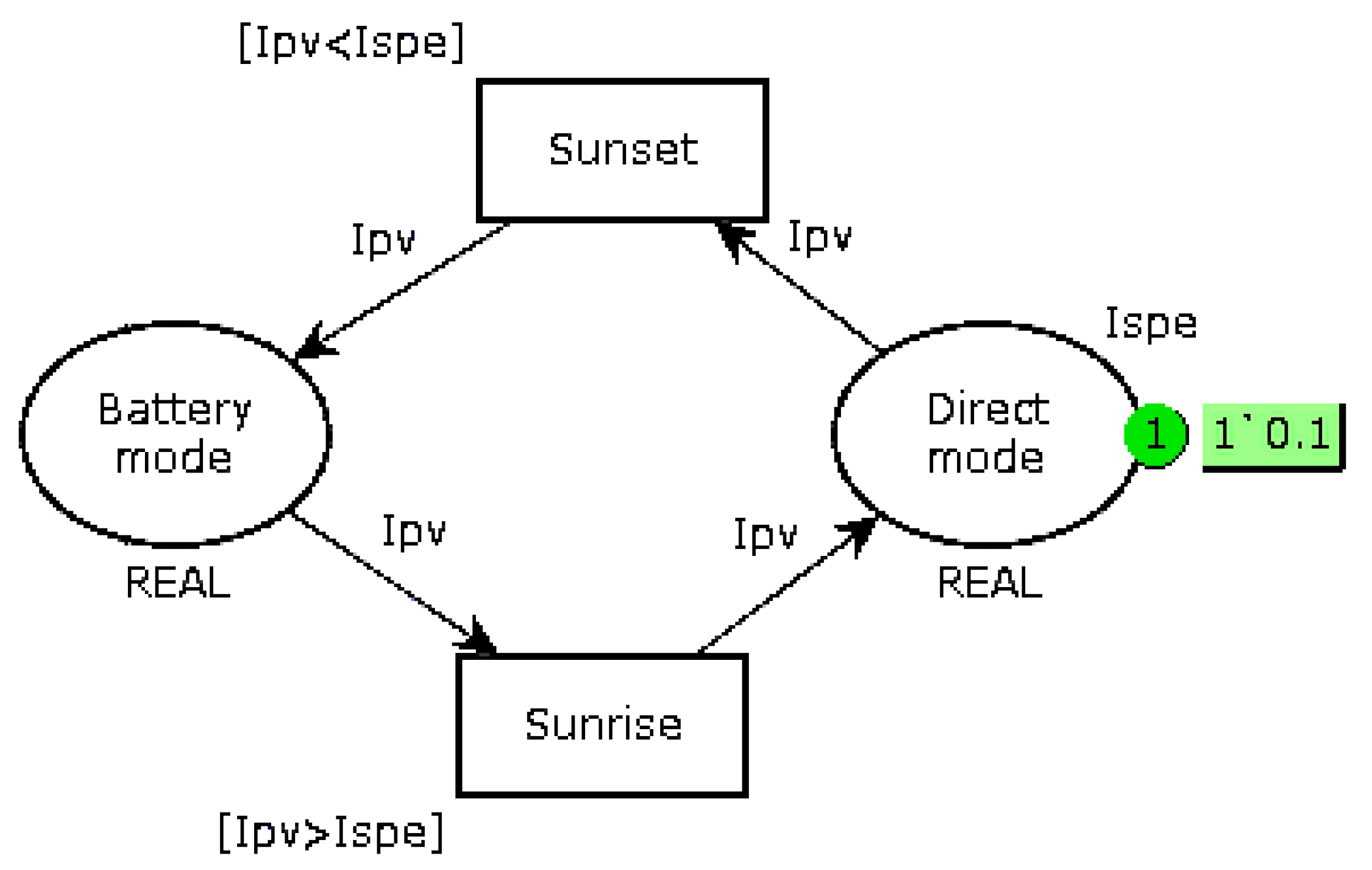
- When the current Ipv from the EHD is greater than the current Ispe requested by the autonomous device, the excess current is sent to the battery. Otherwise, the battery provides the missing current. The system then switches from a Direct mode with possible recharging of the battery to a battery supply mode, with a discharge of the battery under a current less than or equal to the demand. The system operates in two modes, as shown in Figure 4;
- PMU uses the CC-CV procedure to recharge the battery, with a switching threshold of 2.3 V per cell and a CV mode voltage of 2.35 V.
To lessen the aging of the battery, we propose to add the following constraints:
- If possible, keep the temperature around 30 °C, and otherwise limit it to a value close to the ambient temperature;
- To control the battery charge:
- perform complete recharges with a temperature between 40 and 50 °C;
- If a battery has not been fully charged for 30 days and the Ipv current is sufficient, shed the device so as to perform a full charge;
- If a full charge has occurred less than 15 days ago and there is a risk of doing another full charge, redirect the excess current to an auxiliary device. By default, this auxiliary device should be a cold lighting system, implanted inside the box;
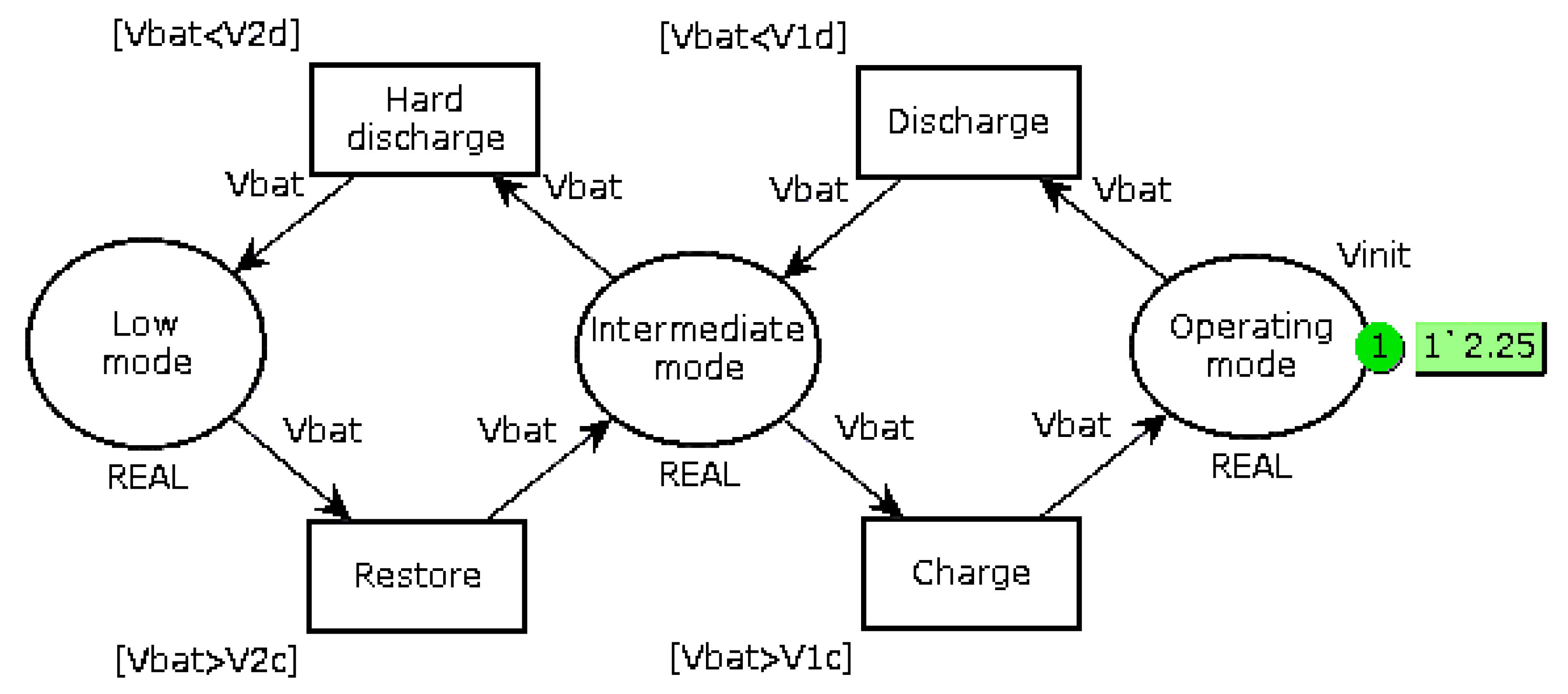
- Replace the bi-modal load-shedding when the battery voltage is less than 12.6 V (6 cells of 2.1 V) by a three-mode operation, as shown in Figure 5. When the voltage is lower than a first threshold V1, the system goes into Intermediate mode, which consists of prioritizing battery recharging and reducing the current supplied to the autonomous device if it can operate in this way. It is also possible to add a mechanical storage system, such as a small flywheel, so as to continue the mission if it requires the nominal current Ispe. When the battery voltage drops below the second threshold V2, a break-contact mechanical relay directly connects the EHD to the battery. The value of these thresholds must be slightly different in recharge and in discharge (V1d, V1c and V2d, V2c) so as to take into account internal relaxation phenomena;
- Monitor the full charge (voltage across a cell greater than 2.35 V). If the voltage reaches this threshold, affect the excess current to the auxiliary device.
In the simulation presented below, the usual functions performed by the PMU, such as the CC-CV charging, are considered effective and do not result in simulation. The complementary improvement of including a small storage system in the autonomous device, such as a flywheel, is not taken into account. We will consider the worst case, which is the one where the device always asks Ispe, including when the system is running in Intermediate mode.
6. Sizing an Example
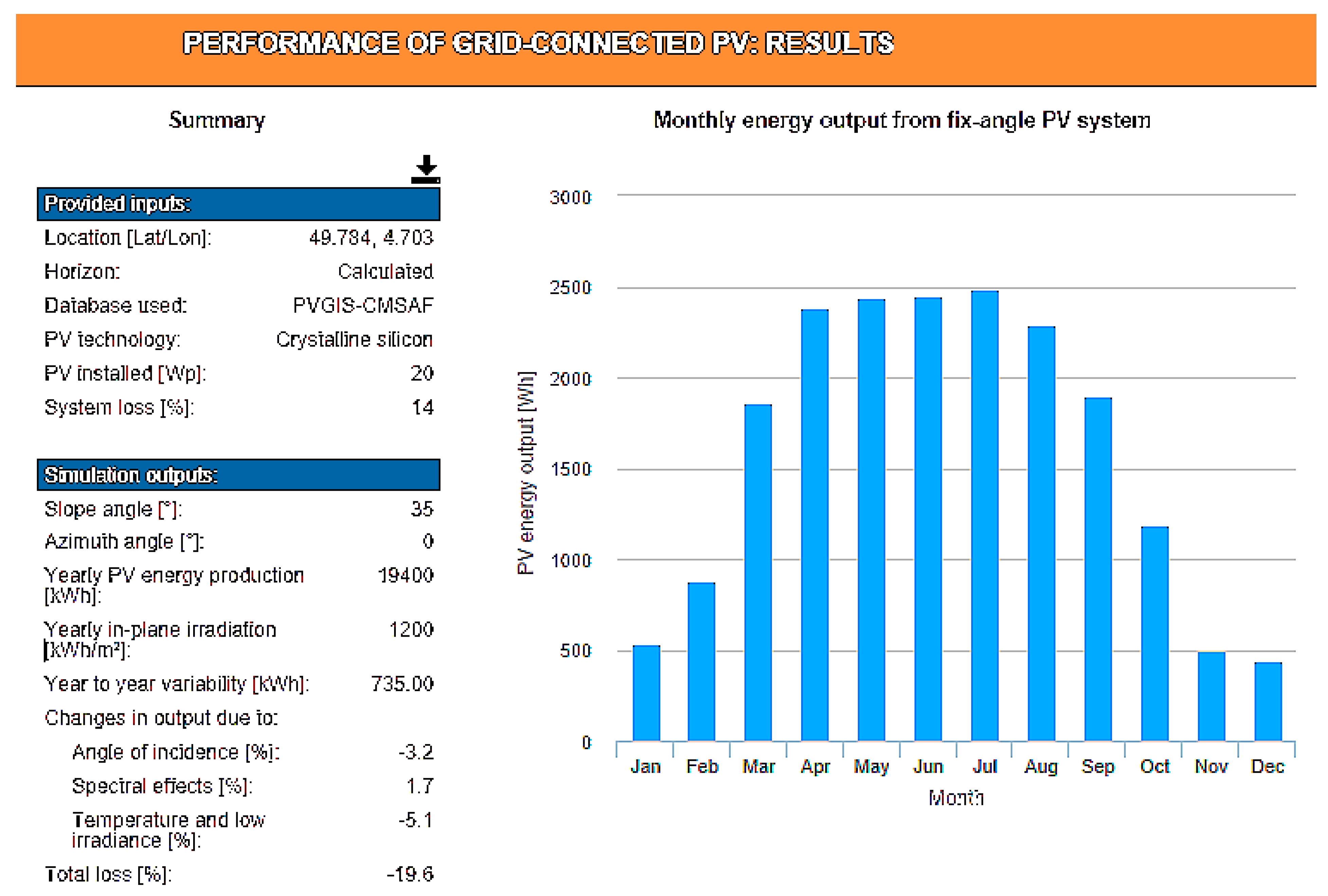
The battery capacity must be calculated so as to avoid a winter failure. Sizing must be made according to the A3PS location and include the usual weather conditions. We take into consideration the coverage of the solar panels by snow for five consecutive days to size our system. During this time, the SoC should not have fallen below 30%, starting from the float capacity. So, we add a safety margin of 5% before the battery goes into deep discharge, corresponding to a cell SoC = 25%. We consider an isolated device, having to work in total autonomy, implanted in the North of France (for example, in Ardennes), which continuously consumes Ispe = 100 mA. This implies a battery capacity greater than 262 Wh. A battery of 12 V–24 Ah satisfies this need. The monthly output of a 20 W-peak PV panel can be determined via the European Commission’s Photovoltaic Geographical Information System (PVGIS) website [27]. For the chosen location, the monthly distribution of the energy collected by an EHV associated with a photovoltaic panel of 20W is specified in Figure 6. Simulation is made for a 30° inclination of a south-facing panel, optimal in France. In December, average production will only be 14 Wh per day. Two panels of this type must be installed in conjunction with a device that disconnects one of the two panels from April to October to reduce the excess energy sent by the EHV in sunny periods. In order for the system to operate with a fan on hot days, it is necessary for the EHV to provide sufficient current. To cool the inside temperature to 2 °C above the outside temperature, it is necessary to have a fan delivering at least 35 m3/h. Any professional fan, operating at a DC voltage of 12 V, 0.6 W, and 87 m3/h of flow is suitable. In the Ardennes, the average maximum temperature is 28 °C and the record is close to 40 °C. To study the worst case, we consider that the box is not completely implanted in the shade and that it requires strong ventilation, which is only reduced in winter.
The system thus fitted makes it possible to operate, even in winter, as shown by Table 1, which includes the self-discharge in the daily energy requirements. The table details the EHV’s monthly and daily average energy production and compares them with the monthly autonomous device associated with the fan consumption. The calculations are made assuming a warm-up all year long during the days of strong sunshine and with a second panel feeding the system the four winter months.
The balance sheet shows two extremes. The first is in winter, when the days have the least amount of sunshine. It is possible that on some days, the battery will not be charged enough to complement the autonomous device needs, which causes a system failure. The second extremum is in July. Hot temperatures associated with high charges will lead to early aging of the battery. Thus, it is sufficient to test the system behavior in December and July and compare the number of failure days for conventional operation in two modes and for operation with the suggested improvement. Table 2 shows the change in luminous flux, expressed in lux, as a function of weather conditions. A cloudy sky reduces the value of sunshine by about half, as well as the production of electrical energy for a solar EHV, since it is directly related to the sunshine degree. Snow accumulated on the ground reduces the energy collected to almost zero. A thunderstorm can be considered as masking the energy collection for three day hours. The A3PS is not established in a tropical zone, so it is also considered that during a rainy day in summer, it is not necessary to ventilate the box. The same principle of summer and winter cycling is included in the standard cycling test IEC 61427 of the International Energy Agency’s IEA PVPS T3-11: 2002, Implementing Agreement on Photovoltaic Power Systems [28], which aims to evaluate the battery lifespan, expressed in terms of capacity loss, by simulating a typical use. It consists of testing the battery in winter conditions, with an SoC varying between 5 and 35% and in summer conditions, with an SoC varying between 75 and 100%. In the simulation carried out here, the constraints imposed lead to an operation, on the one hand, with an SoC between 50% and 100% (conventional PMU) and with an SoC always less than 100% and greater than 25%.
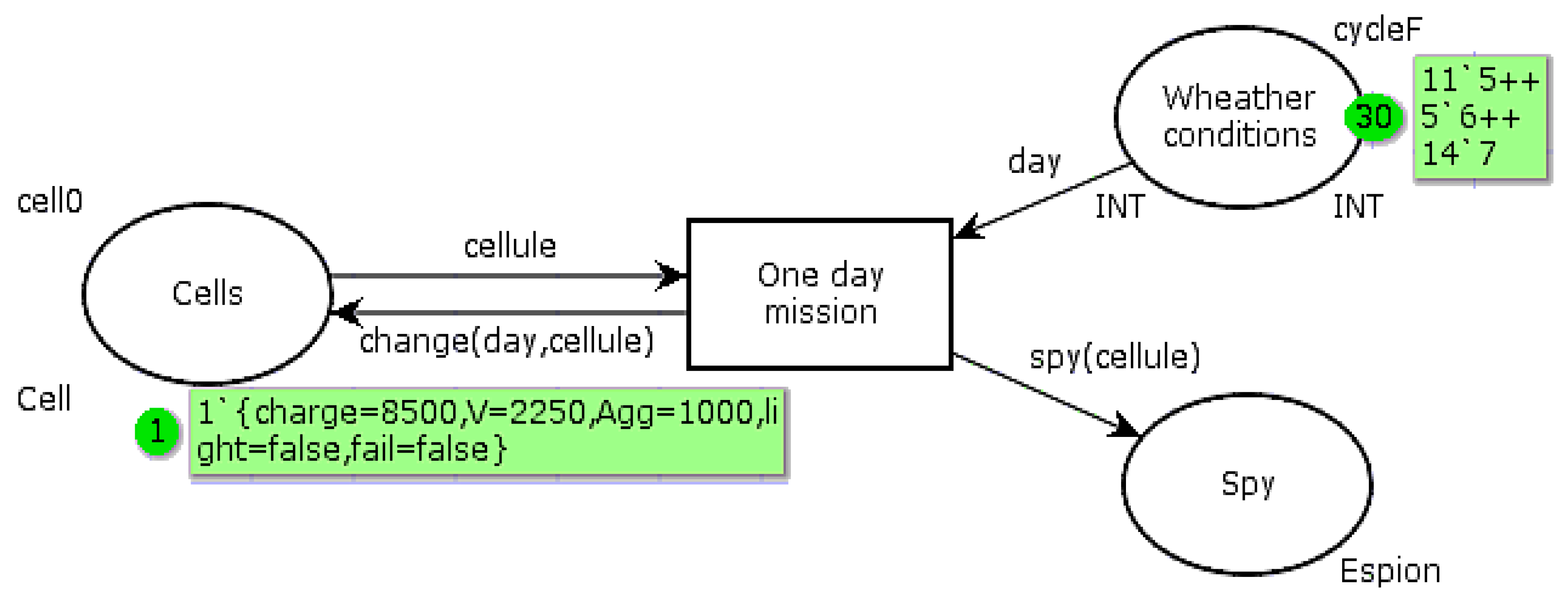
The Figure 7 PN is used to model the system behavior according to whether it works in a conventional manner or with the proposed improvements. The automaton is interested in the cell behavior. It can be resumed to be implanted in the PMU to estimate the cell parameters. “Cell” is a multicolor token, including a color for the electric charge, the OCV, the aggravation rate, the complementary device state, and the mission success. The “Cells” state has an initial marking corresponding to the ideal conditions: float voltage, neutral aggravation rate (Agg = 1), complementary light device extinguished, and mission fulfilled (autonomous device powered by Ispe). The “Weather conditions” state contains a token list “CycleF” simulating the sunshine conditions of each day of the tested month. The days are coded according to the relation (4) coding:
|
The function “change” modifies the marking in the state “Cells” after the transition “One day mission” fire. It is given by algorithm 1. The values introduced in the sub-functions used are those determined in Table 1 and Table 2, expressed in thousandths of units. The “Spy” state is used to display the token list corresponding to the daily cell parameters. The main colors and statements of this PN are given in relations (5). The color “light” is “true” when the complementary device is powered, to keep the battery slightly below the full charge (SoC = 99%). In conventional operation, “light” is always “false”.
|
| Algorithm 1: Influence of a Mission Day on System Parameters |
| fun change(jour:INT,c:Cell) = if (jour = 1) then {{charge = (Downch((#charge(c)),s1,(#fail(c)))), V = Vdown((#charge(c)),s1,(#fail(c))), Agg = (Bas((#charge(c)),s1)), light = Allume((#charge(c)),s1),fail = failure(#charge(c))} else if (jour = 2) then {charge=(Downch((#charge(c)),s2,(#fail(c)))), V = Vdown((#charge(c)),s2,(#fail(c))), Agg = (Bas((#charge(c)),s2)), light = Allume((#charge(c)),s2),fail = failure(#charge(c))} else if (jour = 3) then {charge = Highch((#charge(c)),s3,(#fail(c))), V = Vup((#charge(c)),s3,(#fail(c))), Agg=(Haut((#charge(c)),s3)), light = Allume((#charge(c)),s3),fail = failure(#charge(c))} else if (jour = 4) then {charge = (Downch((#charge(c)),s4,(#fail(c)))), V = Vdown((#charge(c)),s4,(#fail(c))), Agg = (Bas((#charge(c)),s4)), light=Allume((#charge(c)),s4),fail=failure(#charge(c))} else if (jour = 5) then {charge = (Downch((#charge(c)),s5,(#fail(c)))), V = Vdown((#charge(c)),s5,(#fail(c))), Agg = (Bas((#charge(c)),s5)), light = Allume((#charge(c)),s5),fail = failure(#charge(c))} else if (jour = 6) then {charge = Highch((#charge(c)),s6,(#fail(c))), V = Vup((#charge(c)),s6,(#fail(c))), Agg = (Haut((#charge(c)),s6)), light = Allume((#charge(c)),s6),fail = failure(#charge(c))} else {charge = (Downch((#charge(c)),s7,(#fail(c)))), V = Vdown((#charge(c)),s7,(#fail(c))), Agg = (Bas((#charge(c)),s7)), light = false,fail = failure(#charge(c))}; |
The values Si correspond to the daily charge variation of the type i (from 1 to 8) day. It is considered that the weather is invariant on a full day. In the calculation of the aging aggravation parameter, we have considered that, as previously stated, an SoC of less than 0.5 implies an aggravation factor Agg of 1.5 and 2 if SoC < 0.25. The high battery charges also lead to an aggravation factor of 1.5, and then 2, 3, and 4, when the SoC is above the 90%, 95, 99, and 100% thresholds, respectively, in the absence of thermal regulation, so that the convolution of corrosion and evaporation phenomena are taken into account. When the temperature is kept below the outside temperature by more than 2 °C, Agg is 1.5 and 2 beyond the thresholds of 90% and 95%, respectively. The example proposed here exists and has shown two big faults. In the first summer after installation, the temperature in the cabinet was enough to literally melt the PMU. Then, in winter, despite the cessation of the mission for a SoC < 0.5, the battery went into deep discharge and could not be recharged without external intervention.
7. Analysis and Comparisons
The weather of the two extreme months is synthesized in the “weather” columns of Table 3, which also gives the energy produced and the energy balance, in Wh, as well as the variation that it represents with respect to the battery Q0 capacity. The monthly amount of solar energy corresponds to the average indicated by Table 1. In the example used, because of the similarity in daily variations in the battery charge, the type of day 8 (snow) is merged with the type 7 (rain). The initial value “CellF” returns in order the 30 or 31 values of the column “day code” for the month considered.
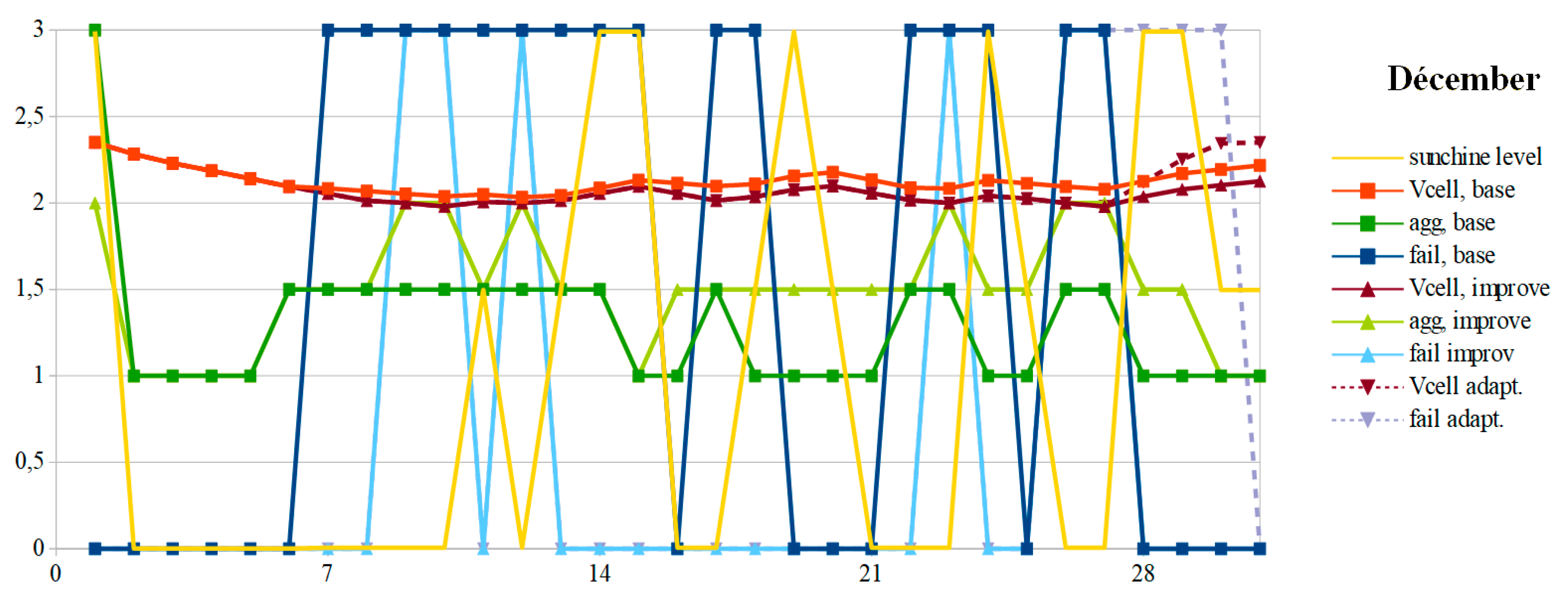
The OCV and the aging aggravation evolution are given, respectively, in Figure 8 and Figure 9 for the months of December and July. In December, the battery OCV with the suggested improvements is permanently lower or equal to that obtained with a conventional PMU. In both cases, due to weather conditions, the mission is often unfilled. This is particularly the case when snow covers the photovoltaic panels or in a durably rainy period. With a dual-mode PMU, the number of failure days is much greater since it stops feeding the autonomous device when the SoC becomes less than 50%. The suggested improvements allow us to divide this number of unavailability days of almost three, in this example. This is at the cost of a lower OCV voltage, which reflects a greater restored energy. To preserve the battery, it is necessary to perform a full charge at least once a month, to the detriment of the autonomous device supplying power. The simulation giving the dashed curves respects this constraint (Vcell_adapt and Failadapt). To achieve this full charge, from December 28, the mission success is set aside to affect all the current Ipv to recharge the battery. When it reaches the full charge, the current is reassigned to the autonomous device. This forced full charge induces an additional three days of failure, but the number of failure days does not reach the number in the conventional solution. If this constraint was not applied, the voltage would follow the violet curve Vcell_improve and the failure according to the cyan curve Failimprove.
Since the battery charge is lower in winter with the suggested improvements, the cells will suffer more from sulphation. Their aging will worsen, by a little more than two thirds in the example. To reduce its impact, the pulsed-current technique should be used during full forced charging. As the battery is not overcharged in winter, the electrodes will not corrode. Advanced techniques such as the dynamic definition of the pulsed-current frequency have been described in [13]. It consists of minimizing the battery impedance, consisting of the ESR in series with the parallel combination of charging resistance with the over-voltage capacity. With this technique, it is necessary to test the full charge and to vary the frequency, depending on the SoC. As a result, corrosion will not be accelerated by these deep discharges.
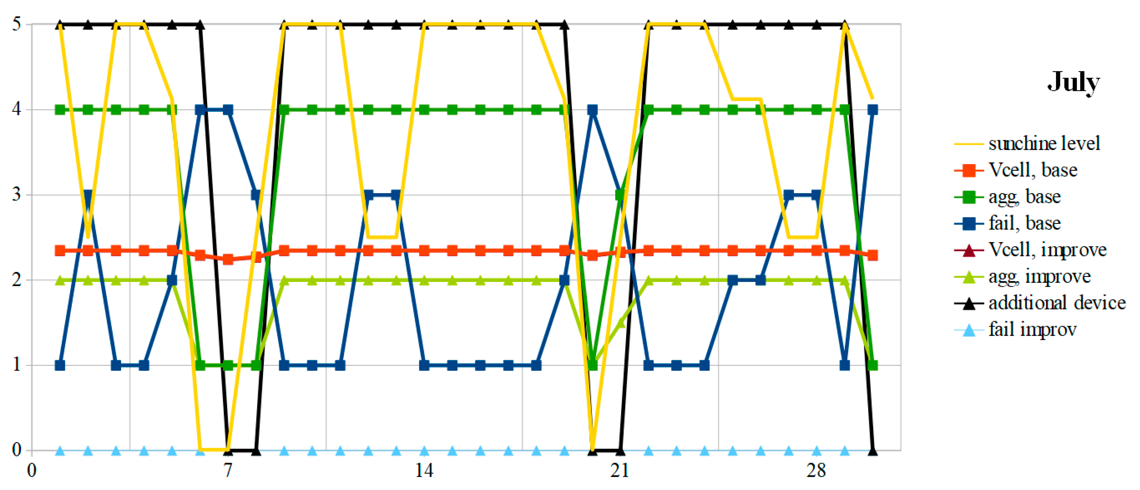
In summer, the battery is often carried in full charge, even if the weather remains rainy for a few days. With a conventional PMU, the battery is almost always overcharged, which accelerates corrosion and aggravates aging. Thanks to the additional device, the battery is never overcharged. It works almost continuously, except during rainy periods. Thus, the battery ages three times slower in summer with the proposed tracks.
A two-dimensional performance indicator can be established by adding, on the one hand, the December and July daily aging aggravations, and on the other hand, the failure days. It is given by relation (6):
The value of this indicator is given in Equation (7):
Overall, over the year, with the suggested improvements, aging aggravation is halved and the number of failure days is reduced more than twice. The aging aggravation due to deeper discharges in winter is offset by the removal of summer full charges, which results in less electrolyte evaporation and more electrode corrosion.
8. Conclusions
Isolated devices can operate in autarky as long as they have a system to capture and store renewable energy. The battery and the energy sensor sizes are sometimes significantly oversized compared to the autonomous device daily energy requirements. Their sizing is often the result of a compromise between the equipment size, failure acceptance (non-power supply of the device), and battery aging. To preserve the batteries, the PMU stops supplying the autonomous device when the SoC drops to 50% in winter, while in summer, the battery is regularly overloaded. Despite this, the battery is often in full charge or heavily discharged when the primary energy source is solar. In this paper, a track to reduce worsening battery aging is proposed. In summer, the battery can thus age less while guaranteeing a greater reliability in winter, by adding a ventilation system, often forgotten in this kind of equipment and tolerated to maintain the mission for battery charges lower than that conventionally admitted in winter. In addition, to reduce sulphation caused by deeper discharges, it is then possible to perform full forced point charges in winter, while ensuring the autonomous device power supply for longer. Ultimately, operating under reduced temperatures but at lower charges increases sulphation, which must be controlled by pulsed currents, while reducing evaporation and without aggravating corrosion.
Author Contributions
Original draft: C.S.; Review and editing: C.S. and E.Y.
Funding
This research received no external funding.
Conflicts of Interest
The authors declare no conflict of interest.
References
- Zairi, S.; Niel, E.; Zouari, B. Global generic model for formal validation of the wireless sensor networks properties. IFAC Proc. Vol. 2011, 44, 5395–5400. [Google Scholar] [CrossRef]
- Rashvand, H.F.; Abedi, A.; Alcaraz-Calero, J.M.; Mitchell, P.D.; Mukhopadhyay, S.C. Wireless sensor systems for space and extreme environments: A review. IEEE Sens. J. 2014, 14, 3955–3970. [Google Scholar] [CrossRef]
- Singh, K.; Moh, S. A comparative survey of energy harvesting techniques for wireless sensor networks. Adv. Sci. Technol. Lett. 2018, 142, 28–33. [Google Scholar]
- Belsky, A.A.; Dobush, V.; Ivanchenko, D. Wind-PV-Diesel Hybrid System with flexible DC-bus voltage level. In Proceedings of the 2014 Electric Power Quality and Supply Reliability Conference (PQ), Rakvere, Estonia, 11–13 June 2014; pp. 181–184. [Google Scholar]
- Yakovleva, E.V.; Skamin, A.N.; Belskiy, A.A. Configuration of a standalone hybrid wind-diesel photoelectric unit for guaranteed power supply for mineral resource industry facilities. Int. J. Appl. Eng. Resour. 2016, 11, 233–238. [Google Scholar]
- Savard, C. Le Stockage de l’Énergie Électrique; Editions Universitaires Europeennes: Paris, France, 2017. [Google Scholar]
- Buckley, D.N.; O’Dwyer, C.; Quil, N.; Lynch, R. Electrochemical Energy Storage. Issues Environ. Sci. Technol. 2019, 45, 115–149. [Google Scholar]
- Stritih, U.; Mlakar, U. Technologies for seasonal solar energy storage in buildings. In Advancements in Energy Storage Technologies; IntechOpen: London, UK, 2018. [Google Scholar] [CrossRef]
- Ruetschi, P. Aging mechanisms and service life of lead-acid batteries. J. Power Sour. 2004, 127, 33–44. [Google Scholar] [CrossRef]
- Bullock, K.R.; Weeks, M.C.; Chalasanik, S.; Murugesamoorthi, K.A. A predictive model of the reliabilities and the distributions of the acid concentrations, open-circuit voltages and capacities of valve-regulated lead/acid batteries during storage. J. Power Sources 1997, 61, 139–145. [Google Scholar] [CrossRef]
- Liaw, B.Y.; Jungst, R.G.; Urbina, A.; Paez, T.L. Modeling of lithium ion cells. A simple equivalent-circuit model approach. Solid State Ionics 2004, 175, 835–839. [Google Scholar]
- El Mehdi, L.; El Filali, A.; Zazi, M. Impact of Pulse Voltage as Desulfator to Improve Automotive Lead Acid Battery Capacity. Int. J. Adv. Comput. Sci. Appl. 2017, 8, 522–526. [Google Scholar] [CrossRef]
- Lam, L.T.; Ozgum, H.; Lim, O.V.; Hamilton, J.A.; Vu, L.H.; Vella, D.G.; Rand, D.A.J. Pulsed-current charging of lead-acid batteries—A possible means for overcoming premature capacity loss. J. Power Sour. 1995, 53, 215–228. [Google Scholar] [CrossRef]
- Chen, L.R. A design of an optimal battery pulse charge system by frequency-varied technique. IEEE Trans. Ind. Electron. 2007, 54, 398–405. [Google Scholar] [CrossRef]
- Mulyono, A.E.; Mustika, T.; Sulaikan, H.P.; Kartini, E. Applications battery performance data acquisition system for monitoring battery performance inside solar cell system. In Proceedings of the 1st Materials Research Society Indonesia Conference and Congress, Yogyakarta, Indonesia, 8–12 October 2018. [Google Scholar]
- Sauer, D.U. Encyclopedia of Electrochemical Power Sources—Secondary batteries: Lead-acid Batteries, Lifetime Determining Processes; Garche, J., Ed.; Elsevier: Amsterdam, The Netherlands, 2009. [Google Scholar]
- Rand, D.A.J.; Moseley, P.T. Lead-acid Battery for Future Automobiles—Lead-acid Battery Fundamentals; Elsevier: Amsterdam, The Netherlands, 2017. [Google Scholar]
- Gauri; Bicht, M.S.; Pant, P.C.; Gairola, P.C. Effect of temperature on flooded lead-acid battery performance. Int. J. Adv. Sci. Res. 2018, 3, 27–29. [Google Scholar]
- Haddad, R.; El Shabat, A.; Kalaani, T. Lead-acid battery modeling for photovoltaic applications. J. Electr. Eng. 2015, 15, 17–24. [Google Scholar]
- Xiong, R.; He, H.; Guo, H.; Ding, Y. Modeling for Lithium-Ion Battery used in Electric Vehicles. Procedia Eng. 2011, 15, 2869–2874. [Google Scholar] [CrossRef] [Green Version]
- Ganesan, A.; Sundaram, S.; Sinkaram, A. Heuristic algorithm for determining state of charge of a lead-acid battery for small engine applications. In Proceedings of the 2012 Small Engine Technology Conference & Exhibition, Madison, WI, USA, 16–18 October 2012. [Google Scholar]
- Goodmin, A. Lead-acid Battery Working—Lifetime Study. Powerthru. 2014. Available online: https://www.scribd.com/doc/305243921/The-Truth-About-Batteries-POWERTHRU-White-Paper (accessed on 10 October 2018).
- Savard, C. Amelioration de la Disponibilite Operationnelle des Systemes de Stockage de L’energie Electrique Multicellulaires. Ph.D. Thesis, Universite de Lyon, INSA de Lyon, French, 2017. [Google Scholar]
- Boufaden, A.; Pietrac, L.; Gabouj, S. L’usage des réseaux de Petri dans la théorie de contrôle par supervision. Available online: https://www.researchgate.net/publication/228449393_L%27usage_des_Reseaux_de_Petri_dans_la_Theorie_de_Controle_par_Supervision (accessed on 10 October 2018).
- Khyzhniak, T.; Kolesnyk, V. Modeling of power-supply subsystems of microgrid using Petri nets. In Proceedings of the Electronics and Nanotechnology (ELNANO), 2013 IEEE XXXIII International Scientific Conference, Kiev, Ukraine, 16–19 April 2013. [Google Scholar]
- Lu, D.; Fakham, H.; Zhou, T.; Francois, B. Application of Petri nets for the energy management of a photovoltaic based power station including storage units. Renew. Energy 2010, 35, 1117–1124. [Google Scholar] [CrossRef]
- European Commission’s Photovoltaic Geographical Information System. Available online: https://photovoltaic-software.com/pv-softwares-calculators/online-free-photovoltaic-software/pvgis (accessed on 10 October 2018).
- Standard Implementing Agreement on Photovoltaic Power Systems—Task 3: Use of Photovoltaic Power Systems in Stand-alone and Island Applications; Report IEA PVPS T3-11; IEA PVPS International Energy Agency: Paris, France, 2002.
Figure 1.
Autonomous system supply principle.

Figure 2.
Linearization of the OCV (SoC) curve (SoC) by parts for a 24 Ah lead-acid cell.

Figure 3.
Colored Petri net example.

Figure 4.
PMU operating modes according to the current coming from the photovoltaic panel.

Figure 5.
Proposed operation of the system in three modes, depending on the cell voltage.

Figure 6.
Monthly energy captured by a 20W solar panel installed in the North of France simulation, from the European Commission PVGIS. [27].
Figure 6.
Monthly energy captured by a 20W solar panel installed in the North of France simulation, from the European Commission PVGIS. [27].

Figure 7.
PN simulating the daily operation and listing the selected parameters.

Figure 8.
Simulated variations in OCV, failure, and aging aggravation, with or without the suggested improvements slopes, in December.
Figure 8.
Simulated variations in OCV, failure, and aging aggravation, with or without the suggested improvements slopes, in December.

Figure 9.
Same curves, in July.


Table 1.
Energy balance between production and consumption in the system.
| Date | Monthly Energy Product (Wh) [27] | Daily Energy Product (Wh) | Daily Consumption (Wh) Device | Daily Consumption (Wh) Fan | Needs | Balance |
|---|---|---|---|---|---|---|
| January | 1068 | 36 | 28.8 | 0.0 | 29.52 | 6.1 |
| February | 1742 | 58 | 28.8 | 0.7 | 30.24 | 27.8 |
| March | 1860 | 62 | 28.8 | 2.9 | 32.40 | 29.6 |
| April | 2380 | 79 | 28.8 | 10.8 | 40.32 | 39.0 |
| May | 2440 | 81 | 28.8 | 13.0 | 42.48 | 38.9 |
| June | 2451 | 82 | 28.8 | 14.4 | 43.92 | 37.8 |
| July | 2491 | 83 | 28.8 | 14.4 | 43.92 | 39.1 |
| August | 2290 | 76 | 28.8 | 14.4 | 43.92 | 32.4 |
| September | 1900 | 63 | 28.8 | 12.2 | 41.76 | 21.6 |
| October | 1190 | 40 | 28.8 | 7.9 | 37.44 | 2.2 |
| November | 992 | 33 | 28.8 | 2.2 | 31.68 | 1.4 |
| December | 900 | 30 | 28.8 | 0.2 | 29.68 | 0.3 |
Table 2.
Energy production rate according to the sunshine.
| Weather Conditions | Brightness (lux) | Energy Production Rate |
|---|---|---|
| Sunrise | 20,000 | 100.00% |
| Clouds | 10,000 | 50.00% |
| Rain | 40 | 0.20% |
| Snow | 4 | 0.02% |
| Storm | 10 | 82.39% (3 h of rain) |
Table 3.
Daily data of simulations on extreme months.
| Day | Weather | Energy Product (Wh) | Balance (Wh) | Charge Change | Day Code | Weather | Energy Product (Wh) | Balance (Wh) | Charge Change | Day Code |
|---|---|---|---|---|---|---|---|---|---|---|
| December | July | |||||||||
| 1 | sunshine | 89.76 | 60.08 | 20.86% | 5 | sunshine | 110.1 | 71.0 | 24.65% | 1 |
| 2 | snow | 0.02 | −29.66 | −10.30% | 8 | clouds | 55.0 | 15.9 | 5.53% | 3 |
| 3 | snow | 0.02 | −29.66 | −10.30% | 8 | sunshine | 110.1 | 71.0 | 24.65% | 1 |
| 4 | snow | 0.02 | −29.66 | −10.30% | 8 | sunshine | 110.1 | 71.0 | 24.65% | 1 |
| 5 | snow | 0.02 | −29.66 | −10.30% | 8 | storm | 90.7 | 51.6 | 17.91% | 2 |
| 6 | snow | 0.02 | −29.66 | −10.30% | 8 | rain | 0.2 | −24.5 | −8.50% | 4 |
| 7 | rain | 0.18 | −29.56 | −10.24% | 7 | rain | 0.2 | −24.5 | −8.50% | 4 |
| 8 | rain | 0.18 | −29.56 | −10.24% | 7 | clouds | 55.0 | 15.9 | 5.53% | 3 |
| 9 | rain | 0.18 | −29.56 | −10.24% | 7 | sunshine | 110.1 | 71.0 | 24.65% | 1 |
| 10 | rain | 0.18 | −29.56 | −10.24% | 7 | sunshine | 110.1 | 71.0 | 24.65% | 1 |
| 11 | clouds | 44.88 | 15.20 | 5,28% | 6 | sunshine | 110.1 | 71.0 | 24.65% | 1 |
| 12 | rain | 0.18 | −29.56 | −10.24% | 7 | clouds | 55.0 | 15.9 | 5.53% | 3 |
| 13 | clouds | 44.88 | 15.20 | 5,28% | 6 | clouds | 55.0 | 15.9 | 5.53% | 3 |
| 14 | sunshine | 89.76 | 60.08 | 20.86% | 5 | sunshine | 110.1 | 71.0 | 24.65% | 1 |
| 15 | sunshine | 89.76 | 60.08 | 20.86% | 5 | sunshine | 110.1 | 71.0 | 24.65% | 1 |
| 16 | rain | 0.18 | −29.56 | −10.24% | 7 | sunshine | 110.1 | 71.0 | 24.65% | 1 |
| 17 | rain | 0.18 | −29.56 | −10.24% | 7 | sunshine | 110.1 | 71.0 | 24.65% | 1 |
| 18 | clouds | 44.88 | 15.20 | 5,28% | 6 | sunshine | 110.1 | 71.0 | 24.65% | 1 |
| 19 | sunshine | 89.76 | 60.08 | 20.86% | 5 | storm | 90.7 | 51.6 | 17.91% | 2 |
| 20 | clouds | 44.88 | 15.20 | 5,28% | 6 | rain | 0.2 | −24.5 | −8.50% | 4 |
| 21 | rain | 0.18 | −29.56 | −10.24% | 7 | clouds | 55.0 | 15.9 | 5.53% | 3 |
| 22 | rain | 0.18 | −29.56 | −10.24% | 7 | sunshine | 110.1 | 71.0 | 24.65% | 1 |
| 23 | rain | 0.18 | −29.56 | −10.24% | 7 | sunshine | 110.1 | 71.0 | 24.65% | 1 |
| 24 | sunshine | 89.76 | 60.08 | 20.86% | 5 | sunshine | 110.1 | 71.0 | 24.65% | 1 |
| 25 | clouds | 44.88 | 15.20 | 5.28% | 6 | storm | 90.7 | 51.6 | 17.91% | 2 |
| 26 | rain | 0.18 | −29.56 | −10.24% | 7 | storm | 90.7 | 51.6 | 17.91% | 2 |
| 27 | rain | 0.18 | −29.56 | −10.24% | 7 | clouds | 55.0 | 15.9 | 5.53% | 3 |
| 28 | sunshine | 89.76 | 60.08 | 20.86% | 5 | clouds | 55.0 | 15.9 | 5.53% | 3 |
| 29 | sunshine | 89.76 | 60.08 | 20.86% | 5 | sunshine | 110.1 | 71.0 | 24.65% | 1 |
| 30 | clouds | 44.88 | 15.20 | 5.28% | 6 | storm | 90.7 | 51.6 | 17.91% | 2 |
| 31 | clouds | 44.88 | 15.20 | 5.28% | 6 | |||||
© 2019 by the authors. Licensee MDPI, Basel, Switzerland. This article is an open access article distributed under the terms and conditions of the Creative Commons Attribution (CC BY) license (http://creativecommons.org/licenses/by/4.0/).
Share and Cite
MDPI and ACS Style
Savard, C.; Iakovleva, E.V. A Suggested Improvement for Small Autonomous Energy System Reliability by Reducing Heat and Excess Charges. Batteries 2019, 5, 29. https://doi.org/10.3390/batteries5010029
AMA Style
Savard C, Iakovleva EV. A Suggested Improvement for Small Autonomous Energy System Reliability by Reducing Heat and Excess Charges. Batteries. 2019; 5(1):29. https://doi.org/10.3390/batteries5010029
Chicago/Turabian StyleSavard, Christophe, and Emiliia V. Iakovleva. 2019. "A Suggested Improvement for Small Autonomous Energy System Reliability by Reducing Heat and Excess Charges" Batteries 5, no. 1: 29. https://doi.org/10.3390/batteries5010029
Note that from the first issue of 2016, this journal uses article numbers instead of page numbers. See further details here.