Article

Ferromagnetic Resonance Studies in Magnetic Nanosystems

by
David S. Schmool
1,*,†,
Daniel Markó
1,†,
Ko-Wei Lin
2,
Aurelio Hierro-Rodríguez
3,4,
Carlos Quirós
3,4,
Javier Díaz
3,4,
Luis Manuel Álvarez-Prado
3,4 and
Jong-Ching Wu
5
1
GEMaC, CNRS, UVSQ, Université Paris-Saclay, 78035 Versailles, France
2
Department of Materials Science and Engineering, National Chung Hsing University, Taichung 402, Taiwan
3
Departamento de Física, Facultad de Ciencias, Universidad de Oviedo, 33007 Oviedo, Spain
4
Centro de Investigación en Nanomateriales y Nanotecnología (CINN), CSIC-Universidad de Oviedo, 33940 El Entrego, Spain
5
Department of Physics, National Changhua University of Education, Changhua 500, Taiwan
*
Author to whom correspondence should be addressed.
These authors contributed equally to this work.
Magnetochemistry 2021, 7(9), 126; https://doi.org/10.3390/magnetochemistry7090126
Submission received: 20 August 2021 / Revised: 7 September 2021 / Accepted: 7 September 2021 / Published: 12 September 2021
(This article belongs to the Special Issue Recent Advances in Nanomagnetism)

Abstract

:
Ferromagnetic resonance is a powerful method for the study of all classes of magnetic materials. The experimental technique has been used for many decades and is based on the excitation of a magnetic spin system via a microwave (or rf) field. While earlier methods were based on the use of a microwave spectrometer, more recent developments have seen the widespread use of the vector network analyzer (VNA), which provides a more versatile measurement system at almost comparable sensitivity. While the former is based on a fixed frequency of excitation, the VNA enables frequency-dependent measurements, allowing more in-depth analysis. We have applied this technique to the study of nanostructured thin films or nanodots and coupled magnetic layer systems comprised of exchange-coupled ferromagnetic layers with in-plane and perpendicular magnetic anisotropies. In the first system, we have investigated the magnetization dynamics in Co/Ag bilayers and nanodots. In the second system, we have studied Permalloy (Ni 80 Fe 20 , hereafter Py) thin films coupled via an intervening Al layer of varying thickness to a NdCo film which has perpendicular magnetic anisotropy.

1. Introduction

Ferromagnetic nanosystems cover a broad range of materials and geometries, which are designed to exploit the intrinsic properties of magnetic materials as well as modify them via structuring, coupling magnetic components (exchange, dipolar, etc.), or a combination of the two [1]. This allows the tailoring of magnetic properties and behavior, which can then be exploited in specific applications, such as magnetic read-heads, data storage systems, or other spintronic devices [2,3]. Research in the area of magnetic materials is wide-ranging and covers extensive areas of materials, experimental methods, theory, and simulations [4,5,6]. In this paper, we will discuss some of the issues concerning nanodot arrays and coupled magnetic layer systems with specific emphasis on the use of magnetization dynamics.
The study of spin dynamics in magnetic systems allows a detailed analysis of the intrinsic and extrinsic properties of magnetic systems [7]. In the former, we include the magnetic properties, such as the magnetization, magnetocrystalline anisotropies, and g-factors of the materials in question. Extrinsic properties arise from the nanostructuring of magnetic film structures as well as from the magnetic interactions between magnetic components of the system in question. For example, the magnetic exchange coupling between ferromagnetic layers will give rise to a modified dynamic response, which depends on the nature and strength of the coupling. Furthermore, reducing the physical dimensions of a magnetic body can cause a number of effects due to magnetic confinement [8,9,10], which can alter the magnetic anisotropy (surface anisotropy) of the material and in certain cases can be manifested as the excitation of standing spin-wave modes, which give rise to multi-peaked FMR spectra.
In this paper, we will present the methodology for the vector network analyzer method for performing ferromagnetic resonance measurements [11]. This technique has been applied to the study of various nanometric systems, such as for nanostructured dot arrays of Co capped with Ag and magnetic layered structures of Py and NdCo separated by a non-magnetic layer of Al. In the latter, the composition of the NdCo has been varied as well as the thickness of the Al layer, which controls the magnetic coupling between the Py and NdCo films.

2. Vector Network Analyzer Ferromagnetic Resonance

In recent years, a number of alternative FMR methods [11,12] have been developed, which have adapted the basic principles of the FMR experiment, making it more suitable for the measurement of nanostructured materials and nanoparticles. Of the methods available, the use of micro-resonators and stripline technologies in tandem with the vector network analyzer (VNA) is extremely promising and has now developed into a well-established method of performing ferromagnetic resonance (VNA-FMR) on thin films and low-dimensional structures. In this technique, the VNA acts as both source and detector, in which the two-port VNA device is connected, via high-frequency cables, to a coplanar waveguide (CPW) or stripline. The use of a planar micro-resonator (PMR) [13] can also increase sensitivity of the measurement, though limits measurements to a fixed frequency, as we will discuss shortly. For the coplanar stripline, there is no resonant cavity, which means that measurements can be made over a broad range of frequencies (commonly referred to as a broadband FMR measurement). In this case, measurements can be made continuously up to tens of gigahertz. The two-port VNA is connected via high-frequency cables to the CPW through which a high-frequency electrical signal is passed from the VNA. The detection is made by measuring the four scattering or S-parameters; these consist of the two transmitted signals (port 1 → port 2, S 21 and port 2 → port 1, S 12 ) and the two reflected signals (port 1 ↔ port 1, S 11 and port 2 ↔ port 2, S 22 ). These four parameters make up the elements of the S-matrix. Since the CPW is impedance-matched (50 Ω ) to the VNA output, this will maximize the transmitted signal, which makes the technique very sensitive to changes in the line impedance. The method requires a full two-port calibration to be implemented to remove background reflections from the cable/waveguide system.
The formal description of the signal obtained by the VNA-FMR method is based on the transmission and reflection coefficients, which are given in the form of the scattering or S-parameters and take into account the line impedance including the sample. These are expressed as lumped elements with the effective inductance ( L ) , series resistance ( R ) , shunt conductance ( G ) , and capacitance ( C ) , and can be expressed as [12,14]:
S 11 = i ω L + R + Z 0 / [ 1 + Z 0 ( G + i ω C ) ] Z 0 i ω L + R + Z 0 / [ 1 + Z 0 ( G + i ω C ) ] + Z 0
and
S 21 = 2 Z 0 / [ 1 + Z 0 ( G + i ω C ) ] i ω L + R + Z 0 / [ 1 + Z 0 ( G + i ω C ) ] + Z 0
where Z 0 is the characteristic impedance of the stripline and ω is the microwave angular frequency. For a symmetric setup, we would expect S 11 = S 22 and S 21 = S 12 . In terms of the complex reflection coefficient, we can write:
Γ = Z Z 0 Z + Z 0
or alternatively we can write:
Z Z 0 = 1 + Γ 1 Γ
where Z is the impedance of the (sample) loaded stripline.
It should be noted that the sensitivity of this method can be limited by the quality of the cables and connectors. Often poor-quality components will introduce further reflections, thus limiting the transmission characteristics of the high-frequency signals. This is particularly true of measurements made at the high-frequency end and above around 40 GHz in general. The magnetic sample, usually in thin-film form, is placed (face-down) on top of the waveguide and located inside the poles of an electromagnet whose field direction should be ideally parallel to the stripline. Placing the sample on the stripline changes the characteristic impedance of the waveguide.
The signal-to-noise ratio is improved by covering as much of the stripline as possible. This can be important for broadband measurements where there is no signal amplification due to Q-factors. The measurement of the FMR spectrum can then proceed in one of two methods: (i) field sweep at a fixed frequency or (ii) frequency sweep with a fixed static magnetic field, H dc . The VNA provides a measurement of the line impedance via transmission and reflection coefficients, which are related to the various S parameters. It should be noted that the electrical signal which passes through the CPW will produce a small oscillating magnetic field, h rf , around the CPW. It is this high-frequency magnetic field that is the driving field for the resonance measurement. As the field or frequency is swept through the resonance of the ferromagnetic sample placed on the CPW, the line impedance will change, hence altering the S-parameters, providing the measurement of the resonance itself. Figure 1 shows a schematic representation of a VNA-FMR setup.
A limitation of the traditional FMR experiment resides in the fact that it must be, by its very nature, a fixed-frequency measurement. The VNA-FMR technique, however, overcomes this problem since it does not require a cavity, and broadband measurements are possible. This, therefore, allows for direct measurement of the frequency–field dispersion relation for a magnetic sample. Excellent agreement with theory is found using this technique, as illustrated in the example of the dispersion relation for a thin Py film, shown in Figure 2.

3. Fundamental Theory of Spin Wave Dispersion in Ferromagnetic Structures

The theory of FMR and more generally spin-wave excitations in ferromagnetic structures has a long history, with major development commencing in the 1950s, with the work of Kittel, Suhl, and co-workers, which in large part derived from the work of Landau and Lifshitz [16] and later Gilbert [17]. In this section, we will provide a summarized introduction to the principal considerations required for the understanding of spin dynamics in low-dimensional structures (thin films and nanostructures). The motion of the magnetization vector can be expressed in a phenomenological form and is frequently given by the Landau–Lifschitz equation, with Gilbert damping also referred to as the LLG equation, and is written as:
1 γ M t = ( M × H eff ) + α γ M s M × M t
Here M and H eff represent the magnetization and effective magnetic field vectors and γ = | e | g / 2 m is the magneto-gyric ratio, in which g is the g-factor. The first term on the right-hand side of Equation (5) can be viewed as the precessional motion of the magnetization vector about the effective magnetic field. The second term concerns the relaxation of this motion and is characterized by the value of α , the Gilbert damping parameter. The combination of the two terms gives rise to a damped precessional motion of M .
The magnetization is comprised of a static and dynamic component; M ( t ) = M 0 + m ( t ) , with the latter arising from the addition of a microwave component, h rf , to the applied magnetic field, H dc . The total (effective) magnetic field, H eff , has several components, which we can express as: H eff = H dc + h rf + H in . For ferromagnetic materials, we need to consider not only the static magnetic field, H dc , and dynamic field, h rf , but also the internal magnetic field, H in , which has a very important role to play in FMR. It will be this internal field component which will provide all the angular dependences due to the various magnetic anisotropies which may exist in the sample; magneto-crystalline anisotropy, shape anisotropy, and surface and interface anisotropy. In a standard FMR experiment, we can make the assumption that the dynamic component of the magnetization is much smaller than the static component; | M 0 | | m | , such that we can neglect second-order effects. This is a valid assumption when the microwave power used is low as in the case of standard microwave spectrometers and vector network analyzers.
Manipulation of the LLG equation via the substitution of the various components of M and H and the expansion of the equilibrium conditions for small-angle deviations, leads to the so-called Smit–Beljers (SB, also known as Smit–Suhl) equation [18,19]:
ω γ 2 = 1 M 2 sin 2 θ 2 E θ 2 2 E ϕ 2 2 E θ ϕ 2
where ω = 2 π f is the angular frequency. This equation neglects damping effects, which will add a small correction to the resonance frequency. Equation (6) uses the second derivatives of the free energy, E, with respect to the polar and azimuthal angles, θ and ϕ , in conjunction with the equilibrium conditions which are defined by the first derivatives of the free energy with respect to the polar and azimuthal angles:
E θ = 0 and E ϕ = 0
These equilibrium conditions define the direction of the magnetization vector under the specific conditions of the free energy density, including all magnetic anisotropies and applied external magnetic fields. The equilibrium (orientation) angles are often designated as θ eq and ϕ eq and the resonance condition will then be evaluated at this orientation. Contributions to the free energy will depend on the magnetic sample under consideration and will in effect be the same contributions that are considered in the effective magnetic field, where we have simply transferred from considering the effective field to considering the total energy of the system. In FMR, the Zeeman energy will always be a principal component due to static and dynamic (microwave) magnetic fields that are required. Additional contributions will also be required and are typically due to magnetostatic (or shape) energy and magneto-crystalline anisotropies. Further manipulation of the LLG Equation (5) [20,21,22] allows for the exchange effects to be considered. This leads to a quadratic equation in ( D k 2 ) of the form:
ω γ 2 = ( D k 2 ) 2 + 1 M 2 E θ 2 + 1 M sin 2 θ 2 E ϕ 2 D k 2 + 1 M 2 sin 2 θ 2 E θ 2 2 E ϕ 2 2 E θ ϕ 2
where D = 2 A ex / M s and k represents the wave vector of the standing spin-wave mode whose allowed values are determined by the boundary (or pinning) conditions, where we have neglected the small correction due to the damping. Evidently for FMR, we can set k = 0 , whereby Equation (8) reduces to Equation (6) for the uniform FMR mode. The extent to which spin-wave terms are important can be principally defined by the exchange stiffness constant, A ex , the boundary conditions [20], and the size of the magnetic entity. In many nanosystems, the size constriction is such that volume modes will not be excited, though arguments for surface modes can be made depending on the boundary conditions permitting surface freedom [23]. We will return to this question at a later stage.
The LLG equation is an intrinsically non-linear expression since the effective field is dependent on the magnetization. In the approximation that we consider under normal experimental conditions, where the dynamic component of the magnetization is small with respect to the static component, we can make an expansion of the variable magnetization in the form of a plane wave, with wave vector ( k ) , such that:
m ( r , t ) = k m k ( t ) e i k · r
Using the contribution of the spatial variation of the magnetization to the time derivative of the magnetization M / t , the dipole-exchange spin-wave dispersion relation for an infinite ferromagnetic medium can be written in the general form as [24]:
ω γ 2 = μ 0 2 ( H + D k 2 ) ( H + D k 2 + M sin 2 θ k )
where θ k defines the angle between the directions of the wave vector and the static magnetization.
For the case, where the film is in the xy plane and the field applied along the x-axis, the resonance equation can be expressed in the form [25]:
ω γ 2 = μ 0 2 ( H + D k 2 ) [ H + D k 2 + M F qq ( k L ) ]
Here, F qq ( k L ) is the matrix element of the magnetic dipole interaction and L denotes the film thickness. In the case of free and perfect pinning, the wave vectors can be expressed in the form:
k 2 = k x 2 + k y 2 + p π L 2 = k 2 + p π L 2
The quantization for the spin waves has the same general pattern of modal number separated by 1 for the two cases. However, for an arbitrary angle between k and M , the matrix elements of the dipole interaction are expressed in a modified form as [25]:
F qq ( k x , k y ) = 1 + P qq ( k ) [ 1 P qq ( k ) ] μ 0 M H + D k 2 k y 2 k 2 P qq ( k ) k x 2 k 2
If the spin wave propagates in the plane of the film, but perpendicular to the external magnetic field ( k z = 0 , k y = k ) , the expression for F qq ( k L ) takes the form:
F qq = 1 + P qq ( k ) [ 1 P qq ( k ) ] μ 0 M H + D k 2
For the lowest value mode, q = 0 , the function P qq ( k ) takes the form:
P 00 ( k ) = 1 + 1 e k L k L
More complex function forms of P qq ( k ) exist for higher mode numbers. If we neglect the exchange, the dispersion relation for the lowest modes results in the so-called Damon–Eshbach (DE) surface magnetostatic modes, expressed in the form:
ω DE γ 2 = μ 0 2 [ H ( H + M ) + M 2 ( 1 e 2 k L ) / 4 ]
When the film is magnetized in the plane with k M , spin-wave modes can be divided into dipole dominated modes ( k = 0 ) , with frequencies expressed in Equation (16), and exchange dominated modes ( k > 0 ) , with frequencies given by the perpendicular standing spin-wave (PSSW) modes:
ω γ 2 = μ 0 2 H + D k 2 + k 2 H + D + H M / H p π / L k 2 + D k 2 + M
For the uniform FMR mode in thin films, the resonance condition can be expressed in the simple Kittel form [26] as:
ω γ 2 = μ 0 2 [ H cos ( θ Θ H ) + M cos 2 θ ] [ H cos ( θ Θ H ) + M cos 2 θ ]
From this, the resonance field is obtained, and therefore Equation (18) can be used to fit angle-dependent FMR measurements, once the equilibrium conditions of the magnetization have been determined from the free energy of the system.
In the simple case of a single magnetic thin film, we can consider the allowed wave vectors for the standing spin wave modes via a simple model, where we reduce the wave vector to the direction (1D) perpendicular to the film plane. For the cases of perfect pinning and free pinning conditions, the wave vectors are generated for the p th mode as:
k ( pp ) = p π L
and
k ( fp ) = ( p 1 ) π L
Intermediate or partial pinning is more complex since the surface spins have a freedom which differs from zero (perfect pinning) and bulk freedom (free pinning). We can introduce a pinning factor, δ , which allows us to vary the pinning, such that:
k ( part ) = ( p δ ) π L
From Equation (21) we can see that the two limiting cases of perfect pinning and freedom can be obtained for values of δ = 0 and δ = 1 , respectively. Thus we can write that for intermediate pinning 0 < δ < 1 . The case of asymmetric pinning can also be considered. In this case, we can write:
k ( asym ) = p 1 2 ( δ 1 + δ 2 ) π L
The values of δ 1 and δ 2 conform to the limits of δ given above. This general case is seen to be coherent with the general representation, so for the case of symmetric pinning; δ 1 = δ 2 = δ and Equation (21) is re-established. For the case of surface localized modes, where the surface freedom exceeds the bulk value, the wave vector becomes imaginary, k i τ , where τ is a real number, and the mode profile will be such that the surface spins precess with a greater amplitude than bulk spins.
The existence of spin-wave modes in the resonance spectra is manifested by multiple absorption peaks in the FMR spectrum. The uniform or FMR mode will be shifted from its normal value, to a lower field, and the higher-order spin-wave modes are located at fields below that of the uniform mode. For the case of localized or surface modes, the resonance lines are shifted to higher field values with respect to the lowest spin-wave mode. A comprehensive account of higher-order spin-wave modes has been treated in [23].

4. Results and Discussion

4.1. Co/Ag Bilayers and Nanodots

Samples of 50 nm thick Co thin films were deposited on thermally oxidized silicon wafer substrates by Ion Beam Assisted Deposition (IBAD) [27]. During deposition, a Kaufmann ion source operating at 800 V and 7.5 mA was used to sputter the Co target. The base vacuum and deposition pressure were 6.7 × 10 5 Pa and 4 × 10 3 Pa, respectively. After the Co deposition, a 30 nm thick Ag capping layer was subsequently deposited without breaking the vacuum. A combination of electron beam lithography and ion milling was then used to pattern the Co/Ag thin film into a 0.5 × 0.5 mm 2 nanodot array with an individual dot diameter of about 200 nm and a pitch of 400 nm. In Figure 3, we show scanning electron micrographs of a typical nanodot array at three different magnifications.
To better understand the nature of the VNA-FMR data, we use a continuous thin film with the same thickness profiles as for the nanodot structures. This serves as a reference from which we can compare the resonance spectra to determine the effect of nanostructuring. In Figure 4, VNA-FMR spectra for both the Co(50 nm)/Ag(30 nm) bilayer and nanostructured dots are shown. We will analyze the bilayer sample first and then consider the nanodot sample.
For the bilayer system, we observe two clear resonance lines, which we interpret as arising from the first two perpendicular standing spin-wave (PSSW) modes, with p = 1 and p = 2 . The frequency–field characteristic and extracted data for the continuous thin film are illustrated in Figure 4a,c, respectively. The fits to the data are performed using Equation (10), which for our purposes takes the form:
ω γ 2 = ( μ 0 H + μ 0 M s + D k 2 ) ( μ 0 H + D k 2 )
We then use Equation (21) in the fitting process to determine the relevant wave vectors and hence pinning parameter, δ . For this we have assumed a symmetric pinning, with δ 1 = δ 2 = δ . For the data shown in Figure 4c we obtain δ = 1.1 for p = 1 and δ = 1.4 for p = 2 . The fitting procedure also used the following parameters: M s = 1.08 T, a g-factor of g = 2.04 and an exchange stiffness constant of A ex = 1.0 × 10 11 J·m 1 [28], which is reasonable for a 50 nm thick Co film. The fits shown in Figure 4c are in good agreement with the data and the physical parameters are consistent with the Co film studied. With regards to the pinning conditions, we note that the value for δ is close to unity and is consistent with the almost perfect pinning condition.
We now turn our attention to the results for the nanodot structures. These are shown in Figure 4b,d for the raw and extracted data, respectively. The two resonance lines observed in the continuous thin film also appear to be present in the nanodot sample, though with modified wave vectors, these are shown in blue and red in Figure 4c,d. In addition to these modes, there is a further resonance mode in the nanostructured sample, as seen in the spectra and illustrated by the line in green in Figure 4d. This mode has a significantly weaker absorption, but is more clearly observed in the low frequency and low field range. The shift of resonance fields can be clearly attributed to the effect of nanostructuring. The first line that we can consider is the blue line, which appears to be very close to the corresponding blue line in the continuous film data for the p = 1 mode. The red line is somewhat shifted to smaller resonance frequencies with respect to the continuous film ( p = 2 mode), but otherwise appears to be the same mode, which can be accounted for by a modified wave vector for this mode. Fitting these two lines can be based on the same principles as that for the thin film sample. In the latter, we considered that for a thin film the in-plane wave vectors should be zero since the film is effectively infinite in the film plane: k x , y = ( p x , y δ x , y ) π 2 / L x , y 2 = 0 since L x , y and thus k | | = 0 , see Equation (12). For the case of our circular nanodots, the lateral dimensions, corresponding to the 200 nm diameter, can give rise to pinning conditions at the dot edges and thus we should consider the three-dimensional aspect of magnetic confinement. Using Equation (12), we can take into account the dot geometry and the edge pinning conditions, which we can express in a similar manner to the thin film case, from which we can write:
k 2 = k x 2 + k y 2 + p π L 2 = [ ( p δ d ) 2 + ( q δ d ) 2 ] π d 2 + ( r δ L ) 2 π L 2 = k pqr 2
where δ d denotes the edge pinning conditions and δ L those of the upper and lower interfaces, d is the dot diameter, L the films thickness. In considering the three-dimensional case, we need to account for the mode numbers in three directions, as represented by the integers p , q , and r . We note that Equation (24) considers that the pinning is equivalent in both lateral directions and is symmetric. This is justified for the current geometry, since there is no reason to suppose that there should be any variation of the pinning at the edges of the dot structure. In our calculations, we consider that the in-plane anisotropy is weak and that inter-dot (dipole–dipole) interactions are sufficiently weak that we can neglect their effect.
In the case of the first two bulk (PSSW) modes (i.e., the blue and red lines in Figure 4d), the resonance lines are slightly shifted towards a bulk-like uniform mode, since the origin of this curve is shifted to zero. The principal resonance line (denoted in blue) is very similar to that of the continuous film and can be expected to derive from similar boundary conditions as that of the p = 1 mode in the continuous thin film. The red line is much closer to the principal resonance (blue line) than that for the continuous film, which must be due to the modified boundary conditions for the nanodot structures. Since the lateral dimensions are almost four times greater than the perpendicular (thickness) dimension, we can expect the second term, in general, to dominate for the wave vector, Equation (24). This will not be the case, however, for edge localized modes, since the degree of localization can be such that the in-plane wave vectors can rapidly increase for strong localization. We will discuss this issue shortly. We can express the resonance modes in terms of the quantization numbers p , q , and r, from which we can write the lowest order modes as k 111 , k 211 , k 121 , k 221 , etc. As previously, the quantization numbers are integer and commence at 1. We note that due to the circular symmetry, certain modes will be degenerated; k 121 = k 211 , k 122 = k 212 etc., but k 211 = k 121 k 112 . By analyzing the lowest modes, we can assess which are the ones most likely to correspond to the modes observed in the FMR spectra. Setting n 1 = π 2 / d 2 and n 2 = π 2 / L 2 , from Equation (24) we can write:
k 111 2 = 2 ( 1 δ d ) 2 n 1 + ( 1 δ L ) 2 n 2
k 121 2 = k 211 2 = [ ( 2 δ d ) 2 + ( 1 δ d ) 2 ] n 1 + ( 1 δ L ) 2 n 2
k 112 2 = 2 ( 1 δ d ) 2 n 1 + ( 2 δ L ) 2 n 2
k 221 2 = 2 ( 2 δ d ) 2 n 1 + ( 1 δ L ) 2 n 2
k 122 2 = k 212 2 = [ ( 2 δ d ) 2 + ( 1 δ d ) 2 ] n 1 + ( 2 δ L ) 2 n 2
Before we analyze in more detail the mode ordering, we should note that since the principal resonance line in the nanodot system (blue) can be assumed to derive from the first resonance ( p = 1 ) mode in the continuous film, the additional resonance in the nanodots (indicated in green in Figure 4d) must therefore arise from a localized resonance mode. We conclude this from the fact that this resonance is situated at a higher magnetic field with respect to the principal resonance. This means that the wave vector is imaginary and pushes the resonance field to higher values since D k 2 = D ( i τ ) 2 = D τ 2 . Inserting this into the resonance equation, Equation (23), means that the resonance field is shifted up in value (or alternatively, the resonance frequencies shift down), while normal bulk or PSSW modes are situated at lower fields or higher frequencies. This can be seen from the resonance lines shown in Figure 4. This conclusion is supported by the fact that the mode intensity is significantly weaker than the principal mode, which is to be expected since the modal intensity is proportional to the transversal dynamic magnetization. Using Equation (23), we find a good fit to this (green) resonance for which τ = 2.85 × 10 7 m 1 , see Figure 4d.
To analyze the mode ordering, we first note that n 1 2.47 × 10 14 m 2 and n 2 3.95 × 10 15 m 2 , where we have used d = 200 nm and L = 50 nm, respectively. We therefore see that n 2 > n 1 and can make the second terms in Equation (24) dominate the wave vector. Since we can assume that the upper and lower pinning conditions should be close to those of the thin film, i.e., δ L 1 , we can further simplify the analysis. In effect, this means the second terms for the modes with r = 1 will effectively vanish, for example in Equations (25), (26) and (28), etc. We can reasonably assign mode numbers corresponding to the wave vectors k 111 and k 211 or k 121 to the first two PSSW modes, i.e., the blue and red lines shown in Figure 4d. This is coherent with the decreased mode separations, with respect to the continuous thin film since this will depend on the first terms in the wave vectors and hence the lateral dimensions of the nanodot. Based on this analysis, we can provide excellent fits to the experimental data, as illustrated in Figure 4d. For the fits we have used the following fit parameters: M s = 1.09 T, a g-factor of g = 2.04 , and an exchange stiffness constant of A ex = 1.0 × 10 11 J·m 1 , which are in agreement with the parameters used in the fits for the continuous thin films. We note that the edge localized mode required a reduced value of the magnetization, M s = 0.82 T. This parameter is important for setting the slope of the linear portion of the curve and may be interpreted as being due to a reduced magnetization at the edges of the nanodots.

4.2. NdCo/Al/Py Layered Structures

Trilayer samples consisting of a 64 nm thick amorphous NdCo x film with PMA and a 10 nm thick polycrystalline Py film with IMA, which are coupled through a nonmagnetic Al spacer, have been deposited via the magnetron sputtering technique. The trilayer structure itself is sandwiched between Al seed and capping layers, all of which have been grown on Si/SiO 2 substrates. The magnetic properties of the coupled thin films can be controlled by two independent parameters. On the one hand, varying the Co concentration (x = 5, 7.5, and 9) in the NdCo x film allows the modification of the strength of its PMA. A maximum has been found for x = 5, whereas higher or lower Co concentrations lead to a gradually weaker PMA, respectively [29,30]. On the other hand, by adjusting the Al spacer thickness (t = 0 nm, 2.5 nm, 5 nm, and 10 nm), the type of coupling between the two magnetic layers can be set to either direct exchange coupling ( t 1.5 nm) or stray field coupling ( t 2.5 nm). In addition to the coupled bi- and trilayers, a series of reference samples, consisting of a single 10 nm thick Py film as well as single 64 nm thick NdCo x films with varying Co concentrations x, has also been prepared. For the remainder of this paper, the coupled trilayers will be named according to their Co concentration and Al spacer thickness as, e.g., X5T10 for a sample based on a NdCo 5 film and a 10 nm thick Al spacer.
The magnetic properties of the samples have been studied using magnetometry (AGM), MOKE, and FMR. In a previous work, we have analyzed the VNA-FMR data of these samples both as a function of the composition and as a function of the Al spacer thickness [31]. Further characterization has been performed using magnetic force microscopy (MFM). Indeed, these measurements show that the remnant state of the sample has a marked stripe domain pattern, with a periodicity of around 140 nm. This stripe domain pattern has been shown to originate in the NdCo layer and is replicated in the coupled Py film. In our previous study, we presented data for the in-plane FMR with the external magnetic field H dc 
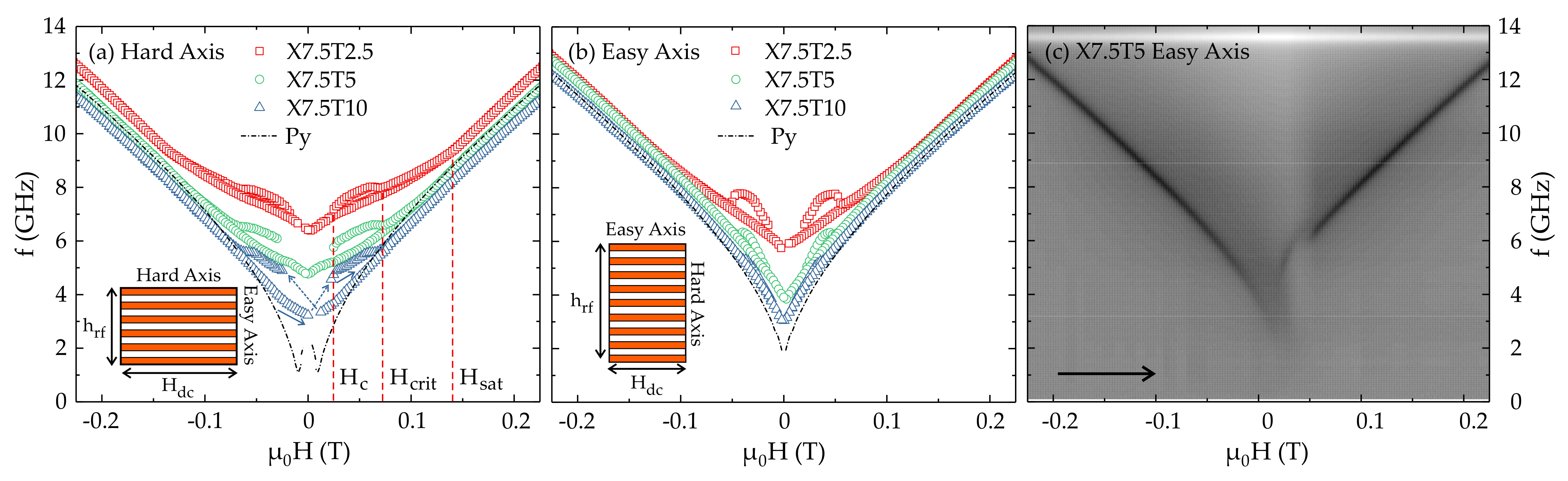
applied along the in-plane hard axis of the samples. We now present the comparison of the in-plane easy and hard axis measurements for samples with a composition value of x = 7.5 . The experimental FMR data are displayed in Figure 5.
In this study, we note that the FMR signal comes solely from the Py layer and no explicit resonance is observed for the NdCo film. The FMR measurements were performed in a specific manner to enable us to correctly interpret and reproduce data. Prior to the FMR measurements, the samples were saturated with a static in-plane magnetic field of H dc = +0.9 T along their easy or hard axis, respectively, i.e., along the direction of the actual measurement. We then perform a full hysteresis cycle from +0.3 T to −0.3 T and then back to +0.3 T in steps of 2.5 mT. Since the spectra only show the Py FMR, we also show the FMR line for a single uncoupled Py film of the same thickness, as shown by the dash-dotted line in Figure 5a,b. This is useful since it also gives a reference line for comparison with the FMR of the coupled Py layers. We note that the single Py film has a small in-plane anisotropy, which we estimate from the graph to give an anisotropy field of around H k = 2 K u / μ 0 M s = 9 mT. We also note that the initial domain pattern after saturation are stripe domains, which are oriented in a direction parallel to H dc . Indeed, it is due to this characteristic that the sample system exhibits a reconfigurable anisotropy. We use the Py FMR as a method to probe the properties and the effect of the NdCo layer due to the magnetic coupling between the two ferromagnetic materials.
There are a number of important observations that we can make before considering a more detailed analysis. Firstly, we note that for the sample series under consideration, the non-magnetic Al spacer thickness allows us to vary the strength or the magnetic coupling between the NdCo 7.5 and Py layers. As the thickness increases, the coupling will reduce, and the Py layer characteristics will be expected to approach those of the isolated film (dashed line). This is roughly what can be observed in Figure 5 and is more clearly seen for the easy axis orientation Figure 5b. We have previously shown that the hysteretic behavior of the FMR line is strongly correlated to the hysteretic loop from magnetometry measurements. This allows us to find the coercive field, H c , and the saturation field, H sat , as indicated in Figure 5a, for the X7.5T2.5 sample. A further critical field, H crit , is indicated, which refers to the field at which the two branches of the hysteresis loop meet [31]. The resonance line follows the arrows shown in Figure 5a, where we note that the dashed arrows indicate the transition through zero-field, where the two branches (up-sweep and down-sweep) of the characteristics cross. Figure 5c shows the corresponding raw FMR data for the X7.5T5 sample. In fact, we note that the transition through zero-field is a little more complex than the data points suggest. In the up-swept data shown, the resonance line appears to cross the zero-field and a jump in the resonance line occurs for small positive fields. This branch then increases and joins the uniform FMR line at the critical field. The down-swept line has lower values of resonance frequency than the up-swept branch in this field range. This then results in the hysteretic behavior of the resonance frequency. In this region, the resonance line appears to be rather weak. Above H c , the resonance line is more pronounced and gradually joins the principal uniform resonance mode as the field reaches H sat .
For the hard axis measurements, the critical field appears to be independent of the spacer layer thickness, though the hysteresis is strongly influenced by the strength of the magnetic coupling of the Py layer with the NdCo 7.5 underlayer. If we consider the evolution of the FMR fH characteristics for the sample series, as t decreases and the magnetic coupling increases, the FMR branches generally shift to higher frequencies, the saturation fields increase and the hysteresis loops appears to be reduced. We also see from this that the zero-field values are strongly affected by the coupling, and increase significantly from the uncoupled Py data. In considering the free Py layer, we note that the coupled Py film in the trilayers have an induced stripe domain texture, which is responsible for these low field differences in the FMR behavior.
The easy axis data show that while the FMR shifts also follow similar trends to that observed along the hard axis, the shifts are generally smaller and the strength of the hysteresis is inverted with respect to the hard axis. Furthermore, the critical field values appear to decrease with increasing Al thickness. The easy axis data also shows that the FMR characteristics of the coupled Py layers approach those of the single Py film as the Al layer thickness increases and decoupling from the NdCo film increases.
In consideration of the FMR behavior in the regions below the coercive field, we note that FMR measurements are highly sensitive to the relative orientation of the stripe domains and the rf magnetic field. This can lead to acoustic and optical modes, due to in-phase and out-of-phase precession of the magnetization in adjacent stripe domains [32], see Figure 6. As simulated in [33] for a single 200 nm thick Py film, stripe domains and rf magnetic field h rf (dc magnetic field H dc ) are always perpendicular (parallel) during the entire hysteresis cycle and independent of the field sweep direction.
Above saturation, the magnetization of the coupled Py layer will be homogeneous and only the uniform FMR mode is observed. However, for applied magnetic fields lower than the saturation fields, stripe domains can give rise to two FMR modes, an acoustic mode and an optical mode, with the latter having a higher resonance frequency at the same magnetic field. The frequency difference between these modes can be substantial, though manipulation of the films can lead to a significant reduction in the separation of modes [33,34]. However, it should be mentioned that in the coupled trilayers, always just one type of mode is observed when sweeping the bias field H dc from positive to negative saturation and vice versa, with the mode order being always the following: uniform FMR mode → acoustic mode → optical mode → uniform FMR mode.
In order to understand the evolution of the resonance line, particularly in the region below saturation and between positive and negative coercive fields, we need to consider the orientation of the magnetization and the nature of the domain structure from the point of domain nucleation as the applied magnetic field H dc reduces from saturation to field strengths below the coercive field. This is intimately connected to the magnetization loops of the Py film. In the saturated state, the magnetization is rigorously aligned to the external field, with H > H sat . In this domain state, the FMR absorption will rigidly follow the normal uniform mode, as given by the Kittel equation, such as expressed by Equation (23). We know that below both the saturation field and the coercive field, the magnetization can relax from the applied field orientation. In the coupled trilayers, any deviation from the Kittel equation would be indicative of a relaxation of the Py magnetization from the applied field direction, though the Py layer remains in a stripe domain state. Only below the coercive field does domain nucleation occur and the sample enters a multidomain state. For a stripe domain system, such as observed in Py coupled to NdCo, the relative sizes of the oppositely aligned domains will vary, as illustrated schematically in Figure 7. These oppositely aligned domains will undergo FMR in either the acoustic or optical modes, as shown previously in Figure 6, which occur at different magnetic fields (or frequencies).
From the hard axis data, see Figure 5, we note that the resonance line continues without deviation, on passing through H c , suggesting that the acoustic mode is excited (see Figure 8a). The resonance line continues undeviated on passing through zero-field. However, once the positive coercive field is reached, + H c , there is an abrupt jump in the resonance line, as indicated by the red arrow in Figure 8b. At this point in the field sweep, the sample is by definition in a state with equal volumes of the two magnetic domains. To understand the jump in the resonance line, we suggest that at this point the acoustic mode is suppressed and the optical mode becomes visible. For equal volumes of oppositely aligned domains, we expect the transverse magnetization to be zero, so at the exact value of H = + H c , the absorbed intensity will be zero. However, any further increase in H will bring about an increase in the positive domains with respect to the negatively pointing domains, and the transverse magnetization will be non-zero and thus an optical mode can be observed (see Figure 8a). We can resume this scenario in Figure 9, in which we follow the FMR hysteresis from negative to positive fields.
If we consider the resonance equation for the acoustic and optical excitations, we can adapt the FMR equation for the effective wave vectors associated with these modes. Since the in-phase, acoustic excitation follows from the uniform mode, we can consider a value of k ac = 0 , while the optical mode should have a k-vector given by k opt = 2 π / Λ D , where Λ D corresponds to the periodicity of the stripe domain texture. We can now consider the frequency shift at H = H c as deriving from the resonance equations for these two excitations. Thus we can write:
Δ f = f opt f ac = μ 0 γ 2 ( 2 H c + M ) D k opt 2 + γ 2 ( D k opt 2 ) 2 4 π 2 ( f opt + f ac ) ,
where f opt and f ac are defined in Figure 9. Given that the wave vector for the optical mode must physically correspond to a real value, we can express the optical mode wave vector from Equation (30) as:
k opt 2 = 2 π Λ D 2 = μ 0 2 ( 2 H c + M ) 2 + 16 π 2 Δ f ( f opt + f ac ) / γ 2 μ 0 ( 2 H c + M ) 2 D
This allows us to directly assess the domain structure periodicity (at H = H c ), and if we require, its evolution with increasing field up to the critical field, H crit . Once this field is reached, the sample becomes a single domain, at which k must be zero, and Λ D . Any further increase of the applied field aligns the magnetization along this field direction. The saturation field will bring the system back to rigorous saturation and the uniform FMR mode is recovered. In fact, any difference between the uniform FMR frequency and the actual observed FMR frequency will be due to the misalignment of M and H .
The proposed model, schematically illustrated in Figure 9, depicts the general form of both the magnetization and FMR hystereses. This is in agreement with previous findings [31] and with the data presented in this paper. At this point, we note that our proposed model is made under the assumption that the imprint of the magnetic stripe domain pattern from the NdCo film into the coupled Py layer is strong. However, the strength of interaction between those two magnetic layers varies according to the thickness of the Al spacer. Synchrotron-based experiments are in progress to understand this issue in more detail.
From the fact that the second term in the square root of Equation (31) is much larger than the first, we can simplify the expression and obtain an approximate relation between the stripe domain periodicity and the difference in frequency, Δ f = f opt f ac , such that:
Λ D ( 2 π γ D ) 0.5 [ ( f opt + f ac ) Δ f ] 0.25
The exchange stiffness constant for Py is of the order of A ex = 1.3 × 10 11 J·m 1 [35], which allows us to evaluate the spin wave constant D = 2 A ex / M s . Using a value of M s = 0.7 T (from fits of the in-plane VNA-FMR data of the 10 nm thick Py reference sample), we obtain D = 4.309 × 10 17 T·m 2 . Furthermore, we use γ = g μ B / = 165.33 GHz/T. From the values of f opt = 4.6 GHz and f ac = 3.7 GHz for the hard axis measurement of sample X7.5T10, we calculate the stripe domain periodicity to be Λ D 135 nm. This is in excellent agreement with MFM images for this sample, where the periodicity was found to be around 140 nm.
There is a further element that requires explanation, which concerns the deviation of the FMR line from the uniform FMR line between the saturation and critical fields, as illustrated in Figure 5. Indeed, this deviation is significant for samples with strong coupling between the ferromagnetic layers, i.e., with low Al interlayer thicknesses. This is particularly noticeable in the hard axis measurements, where the deviations are more significant. For the thinnest Al interlayer of t Al = 2.5 nm, there is a very large increase. From the increase of the zero-field frequency for the free Py layer, we can estimate an increase of the resonance frequency in the region of 4.2–4.5 GHz for this sample. For the sample with t Al = 10 nm, this value drops to around 1.0–1.5 GHz. The value of this deviation of the resonance frequency, δ f , should be related to the ferromagnetic coupling strength between the NdCo and Py layers. We can convert these frequencies into effective fields using a simple relation: H eff = δ ω / γ = 2 π δ f / γ . Using the zero-field values for the frequencies, we estimate that the effective coupling field, H eff , between the NdCo and Py layers drops from about 0.4 T to about 0.1 T as the Al interlayer thickness increases from 2.5 nm to 10 nm. This represents a significant ferromagnetic coupling between the layers.

5. Conclusions

Ferromagnetic resonance is an extremely sensitive tool for probing the dynamic magnetic behavior in ferromagnetic nanostructures and allows us to analyze in detail the properties of various types of nanometric systems. This will include a consideration of the dynamic magnetic properties of the system as well as boundary and magnetic coupling effects.
In this paper, we have shown two examples of the application of the VNA method for performing FMR experiments in magnetic nanostructures. In the first case, we use this technique to study the effect of nanostructuring on the dynamic magnetic properties of Co films and in particular the modification of the FMR spectra due to size reduction and edge effects. We show that the FMR for a continuous thin film can be interpreted from the excitation of PSSW modes, from which we can assess the pinning conditions arising at the magnetic boundaries of the upper and lower surface of the magnetic thin film. The effect of nanostructuring is seen to modify the wave vector of the PSSW modes and shifts the resonances accordingly. This arises from a consideration of the lateral confinement effect in the nanodot structure and can be taken into account in the expression of the three-dimensional wave vector. Furthermore, we note that an additional resonance is also observed and can be attributed to the existence of an edge localized resonance, which is due to the edges of the dot itself. The fit to the experimental values requires a small modification of the magnetization, which could also indicate that the edges of the ferromagnetic dots are reduced with respect to the bulk of the dot structure.
The second magnetic system that we have considered here are layered structures consisting of a hard magnetic NdCo film with perpendicular anisotropy coupled to a soft magnetic Py film, which naturally has an in-plane anisotropy. The coupling between the layers is controlled by the thickness of a non-magnetic Al spacer layer. Our FMR data were performed by making both up and down field sweeps from saturation and allowed us to highlight the hysteretic properties of the dynamic response. We have been able to explain the existence of this hysteresis by accounting for the switching of the modes between acoustic and optical resonances that naturally occur in unsaturated systems with different magnetic domains. Since the NdCo layer induces a regular magnetic stripe domain structure in the Py film, we have been able to further interpret the data using a simple model to explain the frequency shift between the modes. This has ultimately been supported by the relation between the frequency shift and the stripe domain periodicity. The calculation of this periodicity gives a value of Λ D 135 nm and is in excellent agreement with MFM domain images, where a periodicity of 140 nm was observed.

Author Contributions

Conceptualization, D.S.S., D.M., K.-W.L. and L.M.Á.-P.; methodology, D.S.S., D.M. and L.M.Á.-P.; formal analysis, D.S.S. and D.M.; investigation, D.S.S., D.M., K.-W.L., A.H.-R., C.Q., J.D. and L.M.Á.-P.; resources, D.S.S., K.-W.L., L.M.Á.-P. and J.-C.W.; data curation, D.M., K.-W.L. and L.M.Á.-P.; writing—original draft preparation, D.S.S.; writing—review and editing, D.S.S., D.M., K.-W.L., L.M.Á.-P. and J.-C.W.; visualization, D.S.S. and D.M.; supervision, D.S.S., K.-W.L. and L.M.Á.-P.; project administration, D.S.S., K.-W.L. and L.M.Á.-P.; funding acquisition, D.S.S., K.-W.L. and L.M.Á.-P. All authors have read and agreed to the published version of the manuscript.

Funding

D.S.S., D.M. and L.M.Á.-P. acknowledge financial support from the Institut de Physique of CNRS for experimental equipment, a post doc position, and guest researcher stays, respectively. A.H.-R. acknowledges European Union’s Horizon 2020 framework program for research and innovation under the Marie Skłodowska-Curie Action No. H2020-MSCA-IF-2016-746958. A.H.-R., C.Q., J.D. and L.M.Á.-P. would like to thank the Spanish Ministerio de Ciencia e Innovación (MCI) for financial support under Project PID2019-104604RB/AEI/10.13039/501100011033. The contributions of F. Valdés-Bango in the initial stage of the NdCo/Py/Al research project are acknowledged.

Institutional Review Board Statement

Not applicable.

Informed Consent Statement

Not applicable.

Data Availability Statement

The data presented in this study are available on request from the corresponding author.

Conflicts of Interest

The authors declare no conflict of interest.

Abbreviations

The following abbreviations are used in this manuscript:
AGMAlternating gradient magnetometry
CPWCoplanar waveguide
dcDirect current
DEDamon–Eschbach
FMRFerromagnetic resonance
IMAIn-plane magnetic anisotropy
LLGLandau–Lifshitz–Gilbert
MFMMagnetic force microscopy
MOKEMagneto-optical Kerr effect
PMAPerpendicular magnetic anisotropy
PSSWPerpendicular standing spin wave
PyPermalloy
rfRadio frequency
SWRSpin-wave resonance
VNAVector network analyzer

References

  1. Bland, J.; Heinrich, B. (Eds.) Ultrathin Magnetic Structures III: Fundamentals of Nanomagnetism; Springer: Berlin/Heidelberg, Germany, 2005. [Google Scholar]
  2. Heinrich, B.; Bland, J. (Eds.) Ultrathin Magnetic Structures IV: Applications of Nanomagnetism; Springer: Berlin/Heidelberg, Germany, 2005. [Google Scholar]
  3. Hirohata, A.; Yamada, K.; Nakatani, Y.; Prejbeanu, I.L.; Diény, B.; Pirro, P.; Hillebrands, B. Review on spintronics: Principles and device applications. J. Magn. Magn. Mater. 2020, 509, 166711. [Google Scholar] [CrossRef]
  4. Heinrich, B.; Bland, J. (Eds.) Ultrathin Magnetic Structures II: Measurement Techniques and Novel Magnetic Properties; Springer: Berlin/Heidelberg, Germany, 1994. [Google Scholar]
  5. Schmool, D.S.; Kachkachi, H. Chapter Four–Single-Particle Phenomena in Magnetic Nanostructures. In Solid State Physics; Academic Press: Waltham, MA, USA, 2015; Volume 66, pp. 301–423. [Google Scholar] [CrossRef]
  6. Schmool, D.; Kachkachi, H. Chapter One–Collective Effects in Assemblies of Magnetic Nanoparticles. In Solid State Physics; Academic Press: Cambridge, MA, USA, 2016; Volume 67, pp. 1–101. [Google Scholar] [CrossRef]
  7. Bland, J.; Heinrich, B. (Eds.) Ultrathin Magnetic Structures I: An Introduction to the Electronic, Magnetic and Structural Properties; Springer: Berlin/Heidelberg, Germany, 1994. [Google Scholar]
  8. Hillebrands, B.; Ounadjela, K. (Eds.) Spin Dynamics in Confined Magnetic Structures I; Springer: Berlin/Heidelberg, Germany, 2002. [Google Scholar] [CrossRef]
  9. Hillebrands, B.; Ounadjela, K. (Eds.) Spin Dynamics in Confined Magnetic Structures II; Springer: Berlin/Heidelberg, Germany, 2003. [Google Scholar] [CrossRef]
  10. Hillebrands, B.; Thiaville, A. (Eds.) Spin Dynamics in Confined Magnetic Structures III; Springer: Berlin/Heidelberg, Germany, 2006. [Google Scholar] [CrossRef] [Green Version]
  11. Kalarickal, S.S.; Krivosik, P.; Wu, M.; Patton, C.E.; Schneider, M.L.; Kabos, P.; Silva, T.J.; Nibarger, J.P. Ferromagnetic resonance linewidth in metallic thin films: Comparison of measurement methods. J. Appl. Phys. 2006, 99, 093909. [Google Scholar] [CrossRef] [Green Version]
  12. Maksymov, I.S.; Kostylev, M. Broadband stripline ferromagnetic resonance spectroscopy of ferromagnetic films, multilayers and nanostructures. Phys. E Low-Dimens. Syst. Nanostruct. 2015, 69, 253–293. [Google Scholar] [CrossRef] [Green Version]
  13. Cansever, H.; Lindner, J. Microresonators and Microantennas—Tools to Explore Magnetization Dynamics in Single Nanostructures. Magnetochemistry 2021, 7, 28. [Google Scholar] [CrossRef]
  14. Ding, Y.; Klemmer, T.J.; Crawford, T.M. A coplanar waveguide permeameter for studying high-frequency properties of soft magnetic materials. J. Appl. Phys. 2004, 96, 2969–2972. [Google Scholar] [CrossRef]
  15. Markó, D.; Schmool, D.S. Université Paris-Saclay, UVSQ, CNRS, GEMaC, Versailles, France. Unpublished work. 2019. [Google Scholar]
  16. Landau, L.D.; Lifshitz, E. On the theory of the dispersion of magnetic permeability in ferromagnetic bodies. Phys. Z. Sowjet. 1935, 8, 153. [Google Scholar]
  17. Gilbert, T. A Lagrangian formulation of the gyromagnetic equation of the magnetic field. Phys. Rev. 1955, 100, 1243. [Google Scholar]
  18. Smit, J.; Beljers, H.G. Ferromagnetic Resonance Absorption in BaFe12O19, a Highly Anisotropic Crystal. Philips Res. Rep. 1955, 10, 113–130. [Google Scholar]
  19. Vonsovskii, S.V. (Ed.) Ferromagnetic Resonance: The Phenomenon of Resonant Absorption of a High-Frequency Magnetic Field in Ferromagnetic Substances. Pergamon. 1966. Available online: https://www.sciencedirect.com/book/9780080110271/ferromagnetic-resonance (accessed on 19 August 2021).
  20. Rado, G.; Weertman, J. Spin-wave resonance in a ferromagnetic metal. J. Phys. Chem. Solids 1959, 11, 315–333. [Google Scholar] [CrossRef]
  21. Maksymowicz, A. Spin-wave spectra of insulating films: Comparison of exact calculations and a single-wave-vector model. Phys. Rev. B 1986, 33, 6045–6053. [Google Scholar] [CrossRef] [PubMed]
  22. Schmool, D.S.; Barandiarán, J.M. Ferromagnetic resonance and spin wave resonance in multiphase materials: Theoretical considerations. J. Phys. Condens. Matter 1998, 10, 10679–10700. [Google Scholar] [CrossRef]
  23. Puszkarski, H. Theory of surface states in spin wave resonance. Prog. Surf. Sci. 1979, 9, 191–247. [Google Scholar] [CrossRef]
  24. Herring, C.; Kittel, C. On the Theory of Spin Waves in Ferromagnetic Media. Phys. Rev. 1951, 81, 869–880. [Google Scholar] [CrossRef]
  25. Kalinikos, B.A.; Slavin, A.N. Theory of dipole-exchange spin wave spectrum for ferromagnetic films with mixed exchange boundary conditions. J. Phys. C Solid State Phys. 1986, 19, 7013–7033. [Google Scholar] [CrossRef]
  26. Farle, M. Ferromagnetic resonance of ultrathin metallic layers. Rep. Prog. Phys. 1998, 61, 755–826. [Google Scholar] [CrossRef]
  27. Li, X.; Alkadour, B.; Chuang, W.C.; Marko, D.; Schmool, D.; Wu, J.C.; Manna, P.K.; Lin, K.W.; van Lierop, J. Temperature evolution of the magnetic properties of Ag/Fe nanodot arrays. Appl. Surf. Sci. 2020, 513, 145578. [Google Scholar] [CrossRef]
  28. Eyrich, C. Exchange Stiffness in Thin-Film Cobalt Alloys. Master’s Thesis, Simon Fraser University, Burnaby, BC, Canada, 2012. [Google Scholar]
  29. Mergel, D.; Heitmann, H.; Hansen, P. Pseudocrystalline model of the magnetic anisotropy in amorphous rare-earth–transition-metal thin films. Phys. Rev. B 1993, 47, 882–891. [Google Scholar] [CrossRef] [PubMed]
  30. Cid, R.; Alameda, J.M.; Valvidares, S.M.; Cezar, J.C.; Bencok, P.; Brookes, N.B.; Díaz, J. Perpendicular magnetic anisotropy in amorphous NdxCo1-x thin films studied by x-ray magnetic circular dichroism. Phys. Rev. B 2017, 95, 224402. [Google Scholar] [CrossRef] [Green Version]
  31. Markó, D.; Valdés-Bango, F.; Quirós, C.; Hierro-Rodríguez, A.; Vélez, M.; Martín, J.I.; Alameda, J.M.; Schmool, D.S.; Álvarez-Prado, L.M. Tunable ferromagnetic resonance in coupled trilayers with crossed in-plane and perpendicular magnetic anisotropies. Appl. Phys. Lett. 2019, 115, 082401. [Google Scholar] [CrossRef]
  32. Ebels, U.; Buda, L.; Ounadjela, K.; Wigen, P.E. Ferromagnetic resonance excitation of two-dimensional wall structures in magnetic stripe domains. Phys. Rev. B 2001, 63, 174437. [Google Scholar] [CrossRef]
  33. Cao, D.; Song, C.; Feng, H.; Song, Y.; Zhong, L.; Pan, L.; Zhao, C.; Li, Q.; Xu, J.; Li, S.; et al. Microwave excitations and magnetization dynamics of stripe domain films. arXiv 2019, arXiv:1903.00656. [Google Scholar]
  34. Cao, D.; Pan, L.; Song, Y.; Cheng, X.; Feng, H.; Zhao, C.; Li, Q.; Xu, J.; Li, S.; Liu, Q.; et al. Influence of the Phase Structure on the Acoustic and Optical Mode Ferromagnetic Resonance of FeNi Stripe Domain Films. In Proceedings of the 2018 IEEE International Magnetics Conference (INTERMAG), Singapore, 23–27 April 2018. [Google Scholar] [CrossRef]
  35. Shull, R.; Kabanov, Y.; Gornakov, V.; Chen, P.; Nikitenko, V. Shape critical properties of patterned Permalloy thin films. J. Magn. Magn. Mater. 2016, 400, 191–199. [Google Scholar] [CrossRef] [PubMed] [Green Version]
Figure 1. Components of a typical VNA-FMR spectrometer: A two-port VNA is connected to a CPW using coaxial cables and end launch connectors. The sample lies in the xy plane face-down on top of the CPW with the x-axis along the CPW. An electromagnet (not shown) generates a static bias field H dc , whereas the microwave current flowing through the CPW generates a weak oscillating field h rf along the y-axis. The four S-parameters that can be detected with such a two-port setup are schematically shown as well.
Magnetochemistry 07 00126 g001
Figure 2. (a) In-plane VNA-FMR data for a 50 nm thick Py film [15] showing the frequency–field characteristics. The color variation shows the absorption intensity. (b) Extracted experimental data (points) from (a) and corresponding fit (line).
Magnetochemistry 07 00126 g002
Figure 3. Planar view SEM images of a Co/Ag nanodot array at (a) 150×, (b) 50,000×, and (c) 200,000× magnification.
Magnetochemistry 07 00126 g003
Figure 4. VNA-FMR spectra for the Co(50 nm)/Ag(30 nm) samples. Raw data for (a) the bilayer sample and (b) the nanostructured dots, extracted data and fits for (c) the bilayer sample and (d) the nanostructured dots. The solid lines are the fits obtained from Equation (23), using the wave vector profiles given in Equation (21).
Magnetochemistry 07 00126 g004
Figure 5. In-plane frequency–field characteristics for VNA-FMR measurements of samples with composition x = 7.5 . The fH characteristics are shown for the hard (a) and easy (b) axis of the sample. The corresponding insets illustrate the field configurations with respect to the in-plane hard and easy axis along with the virgin-state stripe domain pattern, after initial saturation at H dc = + 0.9 T along the in-plane hard or easy axis. (c) Raw VNA-FMR data for the easy axis of sample X7.5T5 for the up-swept field, showing the absorption line discontinuity passing through zero-field.
Magnetochemistry 07 00126 g005
Figure 6. Schematic illustration of the stripe domain pattern for the coupled Py layer illustrating the precessional configurations for the acoustic and optical modes. Black arrows indicate the direction of the x-component of the in-plane magnetization m x in the coupled Py layer inside the stripe domains shown in orange and white color.
Magnetochemistry 07 00126 g006
Figure 7. Schematic illustration of the stripe domain pattern of the coupled Py layer for increasing magnetic field, starting at negative saturation, H sat , and increasing in the positive direction up to + H c < H < + H sat . Black arrows indicate the direction of the x-component of the in-plane magnetization m x in the coupled Py layer, whereas their length is proportional to the magnitude of m x inside the stripe domains. The change of the width of the stripe domains in the direction perpendicular to H dc is, however, largely exaggerated and in reality only very small.
Magnetochemistry 07 00126 g007
Figure 8. (a) Hard axis data of the X7.5 series. Red arrows indicate the field sweep directions with respect to the FMR line hysteresis around zero-field. The suggested modes corresponding to the different field regions of the fH characteristic are also shown. (b) Easy axis frequency–field characteristic of the X5T5 sample for the up-sweep field direction. Critical and coercive fields are also indicated.
Magnetochemistry 07 00126 g008
Figure 9. Schematic illustrations of the in-plane magnetization and in-plane FMR hysteresis loops. In the lower panel, for the MH loop, we indicate the stripe domain patterns, which schematically show the relative sizes of the oppositely aligned magnetic stripe domain structure. The reversible portions (black), as well as the up-sweep (red) and down-sweep (blue) branches of the magnetization reversal loop, are also shown. The corresponding color scheme is also used in the upper panel for the FMR hysteresis. Indicatively shown are the expected acoustic and optical modes.
Magnetochemistry 07 00126 g009
Publisher’s Note: MDPI stays neutral with regard to jurisdictional claims in published maps and institutional affiliations.

