An Interface-Fitted Fictitious Domain Finite Element Method for the Simulation of Neutrally Buoyant Particles in Plane Shear Flow

Abstract

In this paper, an interface-fitted fictitious domain finite element method is developed for the simulation of fluid–rigid particle interaction problems in cases of rotated particles with small displacement, where an interface-fitted mesh is employed for the discrete scheme to capture the fluid–rigid particle interface accurately, thereby improving the solution accuracy near the interface. Moreover, a linearization and decoupling process is presented to release the constraint between velocities of fluid and rigid particles in the finite element space, and to make the developed numerical method easy to be implemented. Our numerical experiments are carried out using two different moving interface-fitted meshes; one is obtained by a rotational arbitrary Lagrangian–Eulerian (ALE) mapping, and the other one through a local smoothing process among interface-cut elements. A unified velocity is defined in the entire domain based on the fictitious domain method, making it easier to develop an interface-fitted mesh generation algorithm in a fixed domain. Both show that the proposed method has a good performance in accuracy for simulating a neutrally buoyant particle in plane shear flow. This approach can be easily extended to fluid–structure interaction problems involving fluids in different states and structures in different shapes with large displacements or deformations.

1. Introduction

Fluid–structure interaction (FSI) is a crucial research field in current engineering applications, see for example [1,2,3,4,5,6,7]. Particle motion in shear flow is a typical representative and has been a hot topic among scholars, with widespread applications in slurry processing [8], colloid separation [9], and biological cell motion [10]. As early as 1922, Jeffery [11] studied the motion of elliptical particles in creeping flow and provided an analytical expression for the relationship between the angular velocity and the angle. Ding and Aidun [12] performed direct numerical simulations using the discrete Boltzmann method to study the motion of elliptical particles in simple shear flow and found that the behavior of particles at low Reynolds numbers agrees well with periodic solutions of Jeffery. Lundell et al. [13] also conducted numerical studies on the motion of an inertial ellipsoid in a creeping linear shear flow of a Newtonian fluid and found that the particle motion is similar to Jeffery’s solution but with the addition of an orbit drift. Furthermore, Pasquino et al. [14] used both experimental and numerical approaches to study the migration and chaining behavior of noncolloidal spheres in a worm-like micellar, viscoelastic solution within the shear flow.

The fictitious domain method is an effective approach for solving FSI problems, which extends the fictitious fluid into solid particles and imposes constraints on their motions in the fluid. Initially proposed by Saul’ev in 1963 [15], the fictitious domain method was used to extend partial differential equations from complex domains to regular ones. Glowinski et al. [16] analyzed the flow around rigid bodies using the fictitious domain method with the Lagrange multiplier in the case of known solid motions. Furthermore, under the assumption that rigid body motions are not known in advance, they directly simulated the flow around moving rigid bodies in two-dimensional and three-dimensional Newtonian and non-Newtonian viscous fluids using the fictitious domain method with the distributed Lagrange multipliers in order to impose constraints on the motion of solid bodies [17]. The distributed Lagrange multipliers-based fictitious domain method for solving fluid–structure interaction problems can also be found in [3,18]. Hwang et al. [19] proposed a novel finite element scheme for direct simulation of the simple shear flow of an inertia-free particle suspension in a Newtonian fluid, applying rigid body conditions on particle boundaries as traction forces through Lagrange multipliers. Yu et al. [4] use the distributed Lagrange multipliers-based fictitious domain method in the simulation of the motion of a spherical particle in a deterministic lateral displacement device. Wang et al. [20] proposed a one-field fictitious domain method for solving general FSI problems, where only fluid variables (velocity and pressure) are defined in the whole domain, while structural variables are no longer defined. This approach not only improves computational efficiency but also maintains the generality and robustness of the distributed Lagrange multiplier-based fictitious domain method.

Nevertheless, the fictitious domain method typically employs a uniformly fixed grid in the entire domain while a moving structural grid on the top of it, which can lead to computational errors near the moving interface as it cannot effectively track the immersed boundary. For example, Auricchio et al. [21] have mentioned that the lack of global regularity in the solution of moving interface problems would cause suboptimal convergence of standard finite element formulation if the computational mesh near the interface is not appropriately modified. Considering the inherent limitations of the fictitious domain method on fixed grids, it seems necessary to introduce grid modification around the interfaces to accurately track moving interfaces and improve computational accuracy. For instance, Wan et al. [22] presented a fictitious boundary method for the simulation of particulate flows, which incorporates the motion of solids and interfaces as additional constraints to the governing Navier–Stokes equations, thereby extending the fluid domain to the entire region. In order to address the issue of low accuracy in boundary approximation, they dynamically relocated the mesh through a special partial differential equation to capture the region near the surface of the moving particles with high accuracy.

In this paper, we develop an interface-fitted fictitious domain method for the simulation of fluid-particle interaction problems. On the one hand, compared with the classical fictitious domain method, our solution accuracy is improved since an interface-fitted mesh is used to track the motion of particles. We note that additional computational efforts to generate the body-fitted mesh are required in this proposed method, and two interface-fitted mesh generation algorithms are given in cases of rotated particles with small displacement. On the other hand, compared to the classical arbitrary Lagrangian–Eulerian (ALE) method, we eliminate the requirement of a fixed number of vertices/elements in the fluid mesh by defining a unified unknown velocity over the entire domain, and instead need to generate an interface-fitted grid in the fixed entire domain. We note that both the classical ALE method and the proposed method can deal with FSI problems in cases of particles with small displacement. But due to the elimination of the requirement of a fixed number of vertices/elements in the fluid, the proposed method is expected to be capable of dealing with FSI problems in cases of particles with large displacement without any remeshing and interpolation.

The rest of this paper is structured as follows. In Section 2, we introduce the model problem of neutral buoyancy particles moving in a planar shear flow. Then, we present the weak formulation based on the fictitious domain method and its ALE description, followed by temporal and spatial discretization, as detailed in Section 3. Numerical results of circular and elliptical particles in planar shear flows are presented in Section 4. The conclusions are reported in Section 5.

2. Model Problems

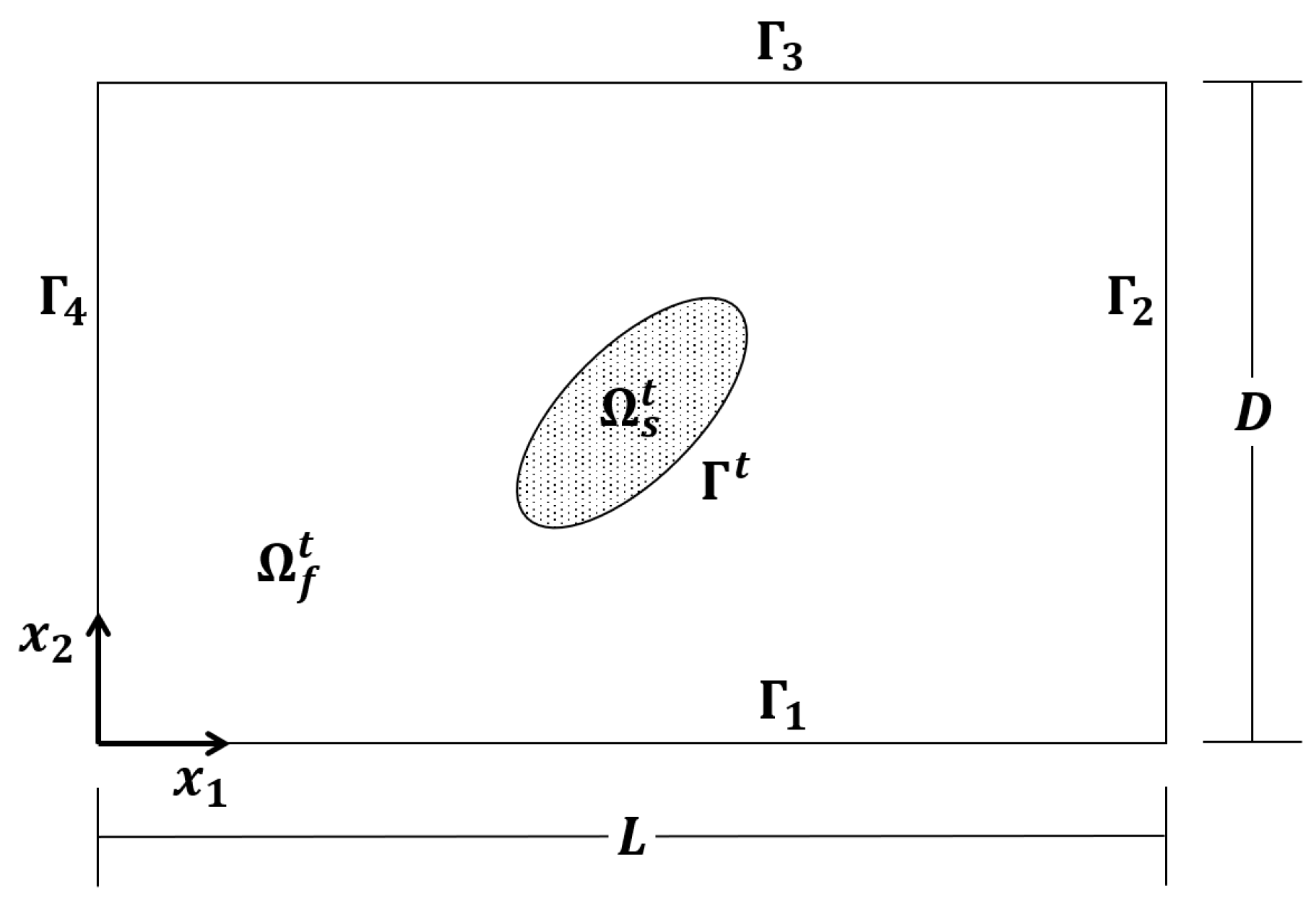
Let $\Omega \in {\mathbb{R}}^2$ be a rectangular domain filled with a Newtonian viscous incompressible fluid and a rigid particle, as depicted in Figure 1. The bottom, right, top and left boundary of $\Omega$ are denoted by ${\Gamma }_1$, ${\Gamma }_2$, ${\Gamma }_3$ and ${\Gamma }_4$, respectively. The distance between ${\Gamma }_2$ and ${\Gamma }_4$ (resp. ${\Gamma }_1$ and ${\Gamma }_3$) is denoted by L (resp. D). For any time $t\in [0,T]$, the interface between fluid and rigid particle is denoted by ${\Gamma }^t$, which divide the domain $\Omega$ into two parts: the fluid domain ${\Omega }_f^t$ and the particle domain ${\Omega }_s^t$.

For the fluid, the governing equations are given by the following Navier–Stokes equations [17],

$$\begin{array}{cc}\hfill {\rho }_f\frac{d{\mathit{u}}_f}{dt}={\rho }_f\mathit{g}+\nabla ·{\sigma }_f,& \hfill \mathrm{in}{\Omega }_f^t\times (0,T],\end{array}$$

(1)

$$\begin{array}{cc}\hfill \nabla ·{\mathit{u}}_f=0,& \hfill \mathrm{in}{\Omega }_f^t\times (0,T],\end{array}$$

(2)

where $\frac{d{\mathit{u}}_f}{dt}=\frac{\partial {\mathit{u}}_f}{\partial t}+({\mathit{u}}_f·\nabla ){\mathit{u}}_f$, ${\mathit{u}}_f$ is the fluid velocity, $\mathit{g}$ is the gravity, ${\sigma }_f=-p\mathit{I}+2{\mu }_f\mathit{D}\left({\mathit{u}}_f\right)$ is the stress tensor with $\mathit{D}\left({\mathit{u}}_f\right)=\frac{1}{2}\left(\nabla {\mathit{u}}_f+{(\nabla {\mathit{u}}_f)}^T\right)$, p is the fluid pressure, ${\rho }_f$ and ${\mu }_f$ are the fluid density and viscosity, respectively. The initial condition is defined as

$${\mathit{u}}_f(\mathit{x},0)={\mathit{u}}_f^0\left(\mathit{x}\right),\mathrm{in}{\Omega }_f^0,$$

(3)

while the boundary conditions are given as follows,

$$\begin{array}{ccc}\hfill {\mathit{u}}_f(\mathit{x},t)=& -{\mathit{g}}_0,\hfill & \hfill \mathrm{on}{\Gamma }_1\times (0,T],\end{array}$$

(4)

$$\begin{array}{ccc}\hfill {\mathit{u}}_f(\mathit{x},t)=& {\mathit{g}}_0,\hfill & \hfill \mathrm{on}{\Gamma }_3\times (0,T],\end{array}$$

(5)

and

$$\begin{array}{ccc}\hfill {\mathit{u}}_f([0,x_2],t)=& {\mathit{u}}_f([L,x_2],t),\hfill & \hfill \forall x_2\in [0,D],t\in (0,T],\end{array}$$

(6)

$$\begin{array}{ccc}\hfill {\sigma }_f{\mathit{n}}_f([0,x_2],t)=& -{\sigma }_f{\mathit{n}}_f([L,x_2],t),\hfill & \hfill \forall x_2\in [0,D],t\in (0,T],\end{array}$$

(7)

where ${\mathit{g}}_0={\left(U_0/2,0\right)}^T$, ${\mathit{n}}_f$ is the outward unit normal vector to the boundary of the fluid domain.

Equations (4) and (5) indicate that the fluid flow field to be studied exhibits characteristics of a shear flow. Such a characteristic arises when velocities of adjacent fluid layers that are parallel to each other are different, which can be attributed to the reinforced boundary conditions. Equations (6) and (7) imply that the fluid velocity is periodic in the $x_1$ direction with the period L, which serves to restore the scenario of unbounded shear flow in the horizontal direction as described in Jeffery’s solution.

The rigid particle motion is defined by the following Euler–Newton’s equations [17] for any $t\in (0,T]$,

$$\begin{array}{cc}\hfill M\frac{d\mathit{U}}{dt}=& M\mathit{g}+\mathit{F}({\mathit{u}}_f,p_f),\hfill \end{array}$$

(8)

$$\begin{array}{cc}\hfill I_{\mathit{G}}\frac{d\omega }{dt}=& T({\mathit{u}}_f,p_f),\hfill \end{array}$$

(9)

$$\begin{array}{cc}\hfill \frac{d\mathit{G}}{dt}=& \mathit{U},\hfill \end{array}$$

(10)

$$\begin{array}{cc}\hfill \frac{d\theta }{dt}=& \omega ,\hfill \end{array}$$

(11)

where $M={\int }_{{\Omega }_s^0}{\rho }_{s}dx$, ${\rho }_s$ and $I_{\mathit{G}}={\int }_{{\Omega }_s^0}{\rho }_s\left({(x_1-G_1)}^2+{(x_2-G_2)}^2\right)d\mathit{x}$, are the mass, density, and moment of inertia of the rigid particle, respectively. $\mathit{G}={\left(G_1,G_2\right)}^T$ is the center of mass, $\mathit{U}$ is the velocity of the center of mass, and, $\omega$ and $\theta$ are the angular velocity and inclination angle of the particle, respectively. Moreover, the hydrodynamical force and torque of the immersed rigid particle are defined as

$$\begin{array}{cc}\hfill \mathit{F}({\mathit{u}}_f,p_f)& =-{\int }_{{\Gamma }^t}{\sigma }_f{\mathit{n}}_{f}ds,\hfill \end{array}$$

(12)

$$\begin{array}{cc}\hfill T({\mathit{u}}_f,p_f)& =-{\int }_{{\Gamma }^t}{\overrightarrow{\mathit{G}\mathit{x}}}^{\perp }·\left({\sigma }_f{\mathit{n}}_f\right)ds,\hfill \end{array}$$

(13)

where ${\overrightarrow{\mathit{G}\left(t\right)\mathit{x}}}^{\perp }={\left(-(x_2-G_2),x_1-G_1\right)}^T$.

The initial conditions for (8)–(11) are defined as

$$\begin{array}{cc}\hfill \mathit{U}\left(0\right)={\mathit{U}}^0,\omega \left(0\right)={\omega }^0,\mathit{G}\left(0\right)=& {\mathit{G}}^0,\theta \left(0\right)={\theta }^0,\hfill \end{array}$$

(14)

where ${\mathit{U}}^0$, ${\omega }^0$, ${\mathit{G}}^0$ and ${\theta }^0$ are given initial values. On the fluid-particle interface ${\Gamma }^t$, the following interface condition is imposed,

$$\begin{array}{cc}\hfill {\mathit{u}}_f(\mathit{x},t)=\mathit{U}\left(t\right)+\omega \left(t\right){\overrightarrow{\mathit{G}\left(t\right)\mathit{x}}}^{\perp },& \mathrm{on}{\Gamma }^t\times (0,T],\hfill \end{array}$$

(15)

which indicates that there is no relative sliding between the fluid and the rigid body.

In summary, all symbols involved in the above model descriptions and their SI units are also listed in

Table 1. Symbol descriptions and their SI units.

Symbols	Description	Units
L	Length of domain	m
D	Width of domain	m
${\mathit{u}}_f$	Fluid velocity	m · s-1
p	Fluid pressure	Pa
$\mathit{g}$	Gravitational acceleration	m · s-2
${\rho }_f$	Density of fluid	kg · m-2
${\mu }_f$	Viscosity of fluid	Pa · s-1
${\rho }_s$	Density of particle	kg · m-2
M	Mass of particle	kg
$\mathit{U}$	Velocity of center of mass	m · s-1
$\mathit{G}$	Position of center of mass	m
$I_{\mathit{G}}$	Moment of inertia of particle	kg · m2
$\omega$	Angular velocity of particle	rad · s-1
$\theta$	Inclination angle of particle	rad
$\mathit{F}$	Hydrodynamic force of particle	N
T	Hydrodynamic torque of particle	N · m

.

3. An Interface-Fitted Fictitious Domain Finite Element Method

3.1. Weak Formulation Based on the Fictitious Domain Method

In this section, we introduce a unified velocity field and present a weak formulation of the aforementioned model problem based on the fictitious domain method.

Introduce Sobolev spaces

$$\begin{array}{cc}\hfill {\tilde{\mathbb{V}}}_f& =\left\{({\mathit{v}}_f,\mathit{V},\xi )\left|{\mathit{v}}_f\in {\left(H^1\left({\Omega }_f^t\right)\right)}^2,\mathit{V}\in {\mathbb{R}}^2,\xi \in \mathbb{R},{\mathit{v}}_f=\mathit{V}+\xi {\overrightarrow{\mathit{G}\mathit{x}}}^{\perp }\mathrm{on}{\Gamma }^t,\right.\right.\hfill \end{array}$$

$$\begin{array}{cc}\hfill & {\mathit{v}}_f=0\mathrm{on}{\Gamma }_1\cup {\Gamma }_3,{\mathit{v}}_f\mathrm{is}\mathrm{periodic}\mathrm{on}{\Gamma }_2\mathrm{and}{\Gamma }_4\},\hfill \end{array}$$

(16)

$$\begin{array}{cc}\hfill Q_f& =\left\{q_f\left|q_f\in L^2\left({\Omega }_f^t\right),{\int }_{{\Omega }_f^t}{q}_{f}d\mathit{x}=0\right.\right\}.\hfill \end{array}$$

(17)

For any $\left({\mathit{v}}_f,\mathit{V},\xi \right)\in {\tilde{\mathbb{V}}}_f$, multiplying both sides of (1) by ${\mathit{v}}_f$, and conducting integration by parts on the stiffness term, we have

$$\begin{array}{cc}\hfill & \begin{array}{cc}\hfill & {\rho }_f{\int }_{{\Omega }_f^t}\frac{d{\mathit{u}}_f}{dt}·{\mathit{v}}_{f}d\mathit{x}+2{\mu }_f{\int }_{{\Omega }_f^t}\mathit{D}\left({\mathit{u}}_f\right):\mathit{D}\left({\mathit{v}}_f\right)d\mathit{x}-{\int }_{{\Omega }_f^t}{p}_f(\nabla ·{\mathit{v}}_f)d\mathit{x}\hfill \\ \hfill & -{\int }_{\partial {\Omega }_f^t}{\mathit{v}}_f·\left({\sigma }_f{\mathit{n}}_f\right)ds={\rho }_f{\int }_{{\Omega }_f^t}\mathit{g}·{\mathit{v}}_{f}d\mathit{x},\hfill \end{array}\hfill \end{array}$$

(18)

where we can rewrite the above boundary integral term as follows by using (8), (9), (12) and (13),

$$\begin{array}{cc}\hfill {\int }_{\partial {\Omega }_f^t}{\mathit{v}}_f·\left({\sigma }_f{\mathit{n}}_f\right)ds& ={\int }_{{\Gamma }_1\cup {\Gamma }_3}{\mathit{v}}_f·\left({\sigma }_f{\mathit{n}}_f\right)ds+{\int }_{{\Gamma }_2\cup {\Gamma }_4}{\mathit{v}}_f·\left({\sigma }_f{\mathit{n}}_f\right)ds+{\int }_{{\Gamma }^t}{\mathit{v}}_f·\left({\sigma }_f{\mathit{n}}_f\right)ds\hfill \\ \hfill & ={\int }_{{\Gamma }^t}\left(\mathit{V}+\xi {\overrightarrow{\mathit{G}\mathit{x}}}^{\perp }\right)·\left({\sigma }_f{\mathit{n}}_f\right)ds=-M\left(\frac{d\mathit{U}}{dt}-\mathit{g}\right)·\mathit{V}-I_{\mathit{G}}\frac{d\omega }{dt}\xi .\hfill \end{array}$$

Thus, for any $({\mathit{v}}_f,\mathit{V},\xi )\in {\tilde{\mathbb{V}}}_f$ and $q_f\in Q_f$, we obtain the following weak formulation of fluid part,

$$\begin{array}{cc}\hfill & \begin{array}{cc}\hfill & {\rho }_f{\int }_{{\Omega }_f^t}\frac{d{\mathit{u}}_f}{dt}·{\mathit{v}}_{f}d\mathit{x}+2{\mu }_f{\int }_{{\Omega }_f^t}\mathit{D}\left({\mathit{u}}_f\right):\mathit{D}\left({\mathit{v}}_f\right)d\mathit{x}-{\int }_{{\Omega }_f^t}{p}_f(\nabla ·{\mathit{v}}_f)d\mathit{x}\hfill \\ \hfill & +M\left(\frac{d\mathit{U}}{dt}-\mathit{g}\right)·\mathit{V}+I_{\mathit{G}}\frac{d\omega }{dt}\xi ={\rho }_f{\int }_{{\Omega }_f^t}\mathit{g}·{\mathit{v}}_{f}d\mathit{x},\hfill \end{array}\hfill \end{array}$$

(19)

$$\begin{array}{cc}\hfill & {\int }_{{\Omega }_f^t}{q}_f(\nabla ·{\mathit{u}}_f)d\mathit{x}=0.\hfill \end{array}$$

(20)

Next, we introduce the particle velocity ${\mathit{u}}_s$, which is defined by

$$\begin{array}{c}\hfill {\mathit{u}}_s=\mathit{U}+\omega {\overrightarrow{\mathit{G}\mathit{x}}}^{\perp }.\end{array}$$

(21)

It is easy to check that

$$\begin{array}{c}\hfill \frac{d{\mathit{u}}_s}{dt}=\frac{d\mathit{U}}{dt}+\frac{d\omega }{dt}{\overrightarrow{\mathit{G}\mathit{x}}}^{\perp }+{\omega }^2\overrightarrow{\mathit{G}\mathit{x}}\end{array}$$

(22)

and

$$\begin{array}{cc}\hfill {\int }_{{\Omega }_s^t}\overrightarrow{\mathit{G}\mathit{x}}d\mathit{x}& ={\int }_{{\Omega }_s^t}(\mathit{x}-\mathit{G})d\mathit{x}={\int }_{{\Omega }_s^t}\left(\mathit{x}-\frac{{\int }_{{\Omega }_s^t}\mathit{x}d\mathit{x}}{{\int }_{{\Omega }_s^t}d\mathit{x}}\right)d\mathit{x}=\mathbf{0},\hfill \end{array}$$

(23)

$$\begin{array}{cc}\hfill {\int }_{{\Omega }_s^t}{\overrightarrow{\mathit{G}\mathit{x}}}^{\perp }d\mathit{x}& ={\int }_{{\Omega }_s^t}{\left(-(x_2-G_2),x_1-G_1\right)}^{\mathrm{T}}d\mathit{x}\hfill \\ \hfill & ={\int }_{{\Omega }_s^t}{\left(-\left(x_2-\frac{{\int }_{{\Omega }_s^t}{x}_{2}d\mathit{x}}{{\int }_{{\Omega }_s^t}d\mathit{x}}\right),x_1-\frac{{\int }_{{\Omega }_s^t}{x}_{1}d\mathit{x}}{{\int }_{{\Omega }_s^t}d\mathit{x}}\right)}^{\mathrm{T}}d\mathit{x}=\mathbf{0}.\hfill \end{array}$$

(24)

For any $\mathit{V}\in {\mathbb{R}}^2$ and $\xi \in \mathbb{R}$, let ${\mathit{v}}_s=\mathit{V}+\xi {\overrightarrow{\mathit{G}\mathit{x}}}^{\perp }$. We have

$$\begin{array}{cc}\hfill {\rho }_s{\int }_{{\Omega }_s^t}\frac{d{\mathit{u}}_s}{dt}·\mathit{V}d\mathit{x}& ={\rho }_s{\int }_{{\Omega }_s^t}\left(\frac{d\mathit{U}}{dt}+\frac{d\omega }{dt}{\overrightarrow{\mathit{G}\mathit{x}}}^{\perp }+{\omega }^2\overrightarrow{\mathit{G}\mathit{x}}\right)·\mathit{V}d\mathit{x}=M\frac{d\mathit{U}}{dt}·\mathit{V},\hfill \end{array}$$

(25)

$$\begin{array}{cc}\hfill {\rho }_s{\int }_{{\Omega }_s^t}\frac{d{\mathit{u}}_s}{dt}·\xi {\overrightarrow{\mathit{G}\mathit{x}}}^{\perp }d\mathit{x}& ={\rho }_s{\int }_{{\Omega }_s^t}\left(\frac{d\mathit{U}}{dt}+\frac{d\omega }{dt}{\overrightarrow{\mathit{G}\mathit{x}}}^{\perp }+{\omega }^2\overrightarrow{\mathit{G}\mathit{x}}\right)·\xi {\overrightarrow{\mathit{G}\mathit{x}}}^{\perp }d\mathit{x}=I_{\mathit{G}}\frac{d\omega }{dt}\xi ,\hfill \end{array}$$

(26)

$$\begin{array}{cc}\hfill {\rho }_s{\int }_{{\Omega }_s^t}\mathit{g}·{\mathit{v}}_{s}d\mathit{x}& ={\rho }_s{\int }_{{\Omega }_s^t}\mathit{g}·\mathit{V}d\mathit{x}+{\rho }_s{\int }_{{\Omega }_s^t}\mathit{g}·\xi {\overrightarrow{\mathit{G}\mathit{x}}}^{\perp }d\mathit{x}=M\mathit{g}·\mathit{V}.\hfill \end{array}$$

(27)

Then for any $\mathit{V}\in {\mathbb{R}}^2$ and $\xi \in \mathbb{R}$, we can attain

$$\begin{array}{c}\hfill {\rho }_f{\int }_{{\Omega }_s^t}\frac{d{\mathit{u}}_s}{dt}·{\mathit{v}}_{s}d\mathit{x}-\frac{{\rho }_f}{{\rho }_s}\left(M\left(\frac{d\mathit{U}}{dt}-\mathit{g}\right)·\mathit{V}+I_{\mathit{G}}\frac{d\omega }{dt}\xi \right)={\rho }_f{\int }_{{\Omega }_s^t}\mathit{g}·{\mathit{v}}_{s}d\mathit{x}.\end{array}$$

(28)

Furthermore, we define a unified velocity

$$\begin{array}{c}\hfill \mathit{u}=\left\{\begin{array}{cc}{\mathit{u}}_f,\hfill & \mathrm{on}{\Omega }_f^t,\\ {\mathit{u}}_s,\hfill & \mathrm{on}{\Omega }_s^t,\end{array}\right.\end{array}$$

(29)

which is defined over the entire domain $\Omega$.

Introduce Sobolev spaces

$$\begin{array}{cc}\hfill \mathbb{V}& =\left\{(\mathit{v},\mathit{V},\xi )\left|\mathit{v}\in {\left(H^1(\Omega )\right)}^2,\mathit{V}\in {\mathbb{R}}^2,\xi \in \mathbb{R},\mathit{v}=\mathit{V}+\xi {\overrightarrow{\mathit{G}\mathit{x}}}^{\perp }\mathrm{on}{\Omega }_s^t,\right.\right.\hfill \end{array}$$

$$\begin{array}{cc}\hfill & \mathit{v}=-{\mathit{g}}_0\mathrm{on}{\Gamma }_1,\mathit{v}={\mathit{g}}_0\mathrm{on}{\Gamma }_3,\mathit{v}\mathrm{is}\mathrm{periodic}\mathrm{on}{\Gamma }_2\mathrm{and}{\Gamma }_4\},\hfill \\ \hfill \tilde{\mathbb{V}}& =\{(\mathit{v},\mathit{V},\xi )\left|\mathit{v}\in {\left(H^1(\Omega )\right)}^2,\mathit{V}\in {\mathbb{R}}^2,\xi \in \mathbb{R},\mathit{v}=\mathit{V}+\xi {\overrightarrow{\mathit{G}\mathit{x}}}^{\perp }\mathrm{on}{\Omega }_s^t,\right.\hfill \end{array}$$

(30)

$$\begin{array}{cc}\hfill & \mathit{v}=0\mathrm{on}{\Gamma }_1\cup {\Gamma }_3,\mathit{v}\mathrm{is}\mathrm{periodic}\mathrm{on}{\Gamma }_2\mathrm{and}{\Gamma }_4\}.\hfill \end{array}$$

(31)

Note that $\frac{d\mathit{u}}{dt}=\frac{\partial \mathit{u}}{\partial t}+(\mathit{u}·\nabla )\mathit{u}$. Thus, by combining (19), (20) and (28), we obtain the final weak formulation of the fluid-particle interaction problem: for any $(\mathit{v},\mathit{V},\xi )\in \tilde{\mathbb{V}}$ and $q_f\in Q_f$, find $(\mathit{u},\mathit{U},\omega )\in \mathbb{V}$ and $p_f\in Q_f$ such that

$$\begin{array}{cc}\hfill & {\rho }_f{\int }_{\Omega }\left(\frac{\partial \mathit{u}}{\partial t}+(\mathit{u}·\nabla )\mathit{u}\right)·\mathit{v}d\mathit{x}+2{\mu }_f{\int }_{{\Omega }_f^t}\mathit{D}\left(\mathit{u}\right):\mathit{D}\left(\mathit{v}\right)d\mathit{x}-{\int }_{{\Omega }_f^t}{p}_f(\nabla ·\mathit{v})d\mathit{x}\hfill \end{array}$$

$$\begin{array}{cc}\hfill & +\left(1-\frac{{\rho }_f}{{\rho }_s}\right)\left[M\left(\frac{d\mathit{U}}{dt}-\mathit{g}\right)·\mathit{V}+I_{\mathit{G}}\frac{d\omega }{dt}\xi \right]={\rho }_f{\int }_{\Omega }\mathit{g}·\mathit{v}d\mathit{x},\hfill \end{array}$$

(32)

$$\begin{array}{cc}\hfill & {\int }_{{\Omega }_f^t}{q}_f(\nabla ·\mathit{u})d\mathit{x}=0,\hfill \end{array}$$

(33)

$$\begin{array}{cc}\hfill M\frac{d\mathit{U}}{dt}& =M\mathit{g}+\mathit{F}(\mathit{u},p_f),\hfill \end{array}$$

(34)

$$\begin{array}{cc}\hfill I_{\mathit{G}}\frac{d\omega }{dt}& =T(\mathit{u},p_f),\hfill \end{array}$$

(35)

subjecting to the following initial conditions

$$\begin{array}{cc}\hfill \mathit{u}& ={\mathit{u}}^0,\mathit{U}={\mathit{U}}^0,\omega ={\omega }^0,\hfill \end{array}$$

(36)

where

$$\begin{array}{c}\hfill {\mathit{u}}^0=\left\{\begin{array}{cc}{\mathit{u}}_f^0,\hfill & \mathrm{in}{\Omega }_f^0,\\ {\mathit{U}}^0+{\omega }^0{\overrightarrow{{\mathit{G}}^{\mathbf{0}}\mathit{x}}}^{\perp },\hfill & \mathrm{in}{\Omega }_s^0.\end{array}\right.\end{array}$$

(37)

For the cases of neutrally buoyant particles, i.e., ${\rho }_s={\rho }_f$, Equation (32) can be simply rewritten as

$$\begin{array}{cc}\hfill & {\rho }_f{\int }_{\Omega }\left(\frac{\partial \mathit{u}}{\partial t}+(\mathit{u}·\nabla )\mathit{u}\right)·\mathit{v}d\mathit{x}+2{\mu }_f{\int }_{{\Omega }_f^t}\mathit{D}\left(\mathit{u}\right):\mathit{D}\left(\mathit{v}\right)d\mathit{x}\hfill \\ \hfill & -{\int }_{{\Omega }_f^t}{p}_f(\nabla ·\mathit{v})d\mathit{x}={\rho }_f{\int }_{\Omega }\mathit{g}·\mathit{v}d\mathit{x}.\hfill \end{array}$$

(38)

3.2. Interface-Fitted Mesh and ALE Mapping

Although the rectangular domain $\Omega$ is independent of time in which the unified velocity $\mathit{u}$ is defined, the fluid-particle interface moves along in time. Thus, we need to construct an interface-fitted mesh in $\Omega$ in order to capture the surface of immersed particle, and therefore improve the accuracy of numerical simulation.

Let N be a positive integer, $\Delta t=T/N$ be the time step and $t^n=n\Delta t$, $n=0,\dots ,N$. Denote by ${\mathcal{T}}_h^n$ a triangulation of ${\Omega }^n:={\Omega }^{t_n}$, where the superscript n indicates the mesh is interface-fitted with ${\Gamma }^{t_n}$. That is, for any edge e in ${\mathcal{T}}_h^n$, $\mathring{e}\cap {\Gamma }_h^{t_n}=\varnothing$, where $\mathring{e}$ denotes the interior of e. For any subdomain D, ${\mathcal{T}}_h^n\left(D\right)$ denotes the restriction of ${\mathcal{T}}_h^n$ on D.

Generally, constructing such interface-fitted meshes and frequent remeshing can lead to prohibitive CPU time in the simulation of FSI problems, especially when the displacement or deformation of the structure is large. In our fictitious domain finite element scheme, the unified unknown velocity is defined in the fixed and connected domain $\Omega$, which releases the requirement that the number of vertices in the fluid subdomain needs to be fixed when an ALE method is used. Although the number of vertices of ${\mathcal{T}}_h^n$ needs to keep fixed, it is much easier to generate an interface-fitted mesh for the entire fixed domain $\Omega$. In fact, some existing moving mesh strategies, such as those in [23,24,25,26], can be employed for generating such interface-fitted background meshes with some slight modifications.

First, in following the idea presented in [26], one can construct an interface-fitted mesh and the corresponding discrete ALE mapping in cases of rotated particles with small displacement, which is called moving mesh Algorithm 1 in this paper, as illustrated in Figure 2 and described below.

Algorithm 1: Moving mesh by a rotational ALE mapping.

1. Draw an artificial circular buffer zone, ${\Omega }_{rf}^t$, in the fluid domain ${\Omega }_f^t$ to enclose the immersed particle ${\Omega }_s^t$ and share the same axis of rotation. Denote ${\Omega }_{sf}^t={\Omega }_f^t\setminus {\Omega }_{rf}^t$, and ${\Gamma }_{rs}^t={\Omega }_{rf}^t\cap {\Omega }_{sf}^t$. 2. Triangulate ${\Omega }_f^0$ with ${\mathcal{T}}_h^0$ that fits ${\Gamma }^0$ and ${\Gamma }_{rs}^0$, i.e., for any edge $e\in {\mathcal{T}}_h^0$, let $\mathring{e}\cap {\Gamma }_{rs}^0=\varnothing$ and $\mathring{e}\cap {\Gamma }^0=\varnothing$. Fix the mesh ${\mathcal{T}}_h^n\left({\Omega }_{sf}^n\right)$ as ${\mathcal{T}}_h^0\left({\Omega }_{sf}^0\right)$ for $n>0$. 3. Rotate ${\mathcal{T}}_h^{n-1}\left({\Omega }_{rf}^{n-1}\right)$ together with the particle at the same angular velocity and about the same axis of rotation to obtain a rotating mesh $\widehat{{\mathcal{T}}_h^n}\left({\Omega }_{rf}^n\right)$. 4. Locally shift the nodes on the artificial interface ${\Gamma }_{rs}$ associated with $\widehat{{\mathcal{T}}_h^n}\left({\Omega }_{rf}^n\right)$ in order to find and match with the fixed coordinates of the closest nodes on ${\Gamma }_{rs}$ associated with ${\mathcal{T}}_h^n\left({\Omega }_{sf}^n\right)$. Thus, the rotating and conforming mesh ${\mathcal{T}}_h^n\left({\Omega }_{rf}^n\right)$, further, the total mesh ${\mathcal{T}}_h^n={\mathcal{T}}_h^n\left({\Omega }_{rf}^n\right)\cup {\mathcal{T}}_h^n\left({\Omega }_{sf}^n\right)$ are obtained.

We note that the discrete ALE-based mesh velocity, $w_h$, only needs to be computed in ${\Omega }_{rf}$, since the mesh ${\mathcal{T}}_h^n\left({\Omega }_{sf}^n\right)$ is fixed. Algorithm 1 guarantees a rigid particle’s vertex of ${\mathcal{T}}_h^0$ (resp. ${\mathcal{T}}_h^0\left({\Omega }_{rf}\right)$) is always the same rigid particle’s vertex of ${\mathcal{T}}_h^n$ (resp. ${\mathcal{T}}_h^n\left({\Omega }_{rf}\right)$) all the time, establishing a one-to-one mapping (denoted by $X_h^n$) between vertices of ${\mathcal{T}}_h^n\left({\Omega }_{rf}\right)$ and of ${\mathcal{T}}_h^0\left({\Omega }_{rf}\right)$.

Next, we present another moving mesh algorithm called Algorithm 2, which is similar to the method proposed in [23].

We remark that Algorithm 2 may deliver such a interface-fitted mesh ${\mathcal{T}}_h^n$ whose rigid particle’s (resp. fluid) vertices at one time step may be fluid (resp. rigid particle’s) vertices at another time step (e.g., see the bottom-right part of Figure 3), but still form a one-to-one discrete ALE mapping between vertices of ${\mathcal{T}}_h^n$ and of ${\mathcal{T}}_h^0$ that is still denoted by $X_h^n$.

Algorithm 2: Moving mesh by local smoothing among interface-cut elements.

1. Triangulate $\Omega$ into a rectangular mesh ${\widehat{\mathcal{T}}}_h$ with a given mesh size $h_x$ (resp. $h_y$) in x-axis (resp. y-axis) direction that is independent of time t. 2. Inspect all vertices of ${\widehat{\mathcal{T}}}_h$ in the column-wise lexicographic order, and divide them into fluid- (black), interface- (red), and rigid particle’s (blue) vertex sets associated with the current position of fluid-particle interface ${\Gamma }^{t_n}$, where the red interface vertices are those vertices closest to ${\Gamma }^{t_n}$, as shown in the top-left part of Figure 3. 3. Move all red interface vertices onto the fluid-particle interface to set them as the closest intersection points between ${\Gamma }^{t_n}$ and ${\widehat{\mathcal{T}}}_h$, respectively. 4. Cut each quadrilateral of ${\widehat{\mathcal{T}}}_h$ with the slash diagonal to obtain a triangular mesh of $\Omega$, ${\tilde{\mathcal{T}}}_h$, where some edges of ${\tilde{\mathcal{T}}}_h$ may intersect with the interface, as shown in the top-right part of Figure 3. 5. Locally adjust interface-cut elements of ${\tilde{\mathcal{T}}}_h$ using vertex smoothing and edge swapping techniques [24] to enhance the mesh quality, simultaneously, ensure the edges of each element are all aligned with the fluid-particle interface ${\Gamma }^{t_n}$. Thus, an interface-fitted mesh ${\mathcal{T}}_h^n$ is generated, as depicted in the bottom-left part of Figure 3.

Once the interface-fitted mesh ${\mathcal{T}}_h^n$ is obtained, the discrete ALE velocity $w_h^n$, which is a piecewise linear function associated with ${\mathcal{T}}_h^n$, can be computed by

$$\begin{array}{c}\hfill {\mathit{w}}_h^n\left(P\right)=\frac{{\mathit{x}}^n\left(P\right)-{\mathit{x}}^{n-1}\left(X_h^{n-1}\circ {\left(X_h^n\right)}^{-1}\left(P\right)\right)}{\Delta t}\end{array}$$

(39)

for any vertex P of ${\mathcal{T}}_h^n$. Moreover, the discrete ALE material derivative is defined as

$$\begin{array}{cc}\hfill {\left.\frac{\partial {\mathit{v}}_h}{\partial t}\right|}_{\widehat{\mathit{x}}}^n:& {\Omega }^n\to {\mathbb{R}}^2\hfill \end{array}$$

(40)

$$\begin{array}{cc}\hfill & (\mathit{x},t^n)\mapsto {\left.\frac{\partial {\mathit{v}}_h}{\partial t}\right|}_{\widehat{\mathit{x}}}^n\left(\mathit{x}\right)={\left(\frac{\partial {\mathit{v}}_h}{\partial t}\right)}^n\left(\mathit{x}\right)+({\mathit{w}}_h^n\left(\mathit{x}\right)·\nabla ){\mathit{v}}_h^n\left(\mathit{x}\right).\hfill \end{array}$$

(41)

Associated with the interface-fitted mesh ${\mathcal{T}}_h^n$, the subdomains ${\Omega }_f^n$ and ${\Omega }_s^n$ are approximated by ${\Omega }_{f,h}^n$ and ${\Omega }_{s,h}^n$, respectively.

3.3. A Interface-Fitted Fictitious Domain Finite Element Method

Define the following finite element spaces

$$\begin{array}{cc}\hfill {\mathbb{V}}_h^n& =\left\{({\mathit{v}}_h,{\mathit{V}}_h,{\xi }_h)\left|{\mathit{v}}_h{|}_K\in {\left(P_2\right)}^2,\forall K\in {\mathcal{T}}_h^n,\right.\right.{\mathit{V}}_h\in {\mathbb{R}}^2,{\xi }_h\in \mathbb{R},{\mathit{v}}_h={\mathit{V}}_h+{\xi }_h{\overrightarrow{{\mathit{G}}_h^n\mathit{x}}}^{\perp }\mathrm{on}{\Omega }_{s,h}^n,\hfill \\ \hfill & {\mathit{v}}_h=-{\mathit{g}}_0\mathrm{on}{\Gamma }_1,{\mathit{v}}_h={\mathit{g}}_0\mathrm{on}{\Gamma }_3,{\mathit{v}}_h\mathrm{is}\mathrm{periodic}\mathrm{on}{\Gamma }_2\mathrm{and}{\Gamma }_4\},\hfill \\ \hfill {\tilde{\mathbb{V}}}_h^n& =\left\{({\mathit{v}}_h,{\mathit{V}}_h,{\xi }_h)\left|{\mathit{v}}_h{|}_K\in {\left(P_2\right)}^2,\forall K\in {\mathcal{T}}_h^n,\right.\right.{\mathit{V}}_h\in {\mathbb{R}}^2,{\xi }_h\in \mathbb{R},{\mathit{v}}_h={\mathit{V}}_h+{\xi }_h{\overrightarrow{{\mathit{G}}_h^n\mathit{x}}}^{\perp }\mathrm{on}{\Omega }_{s,h}^n,\hfill \\ \hfill & {\mathit{v}}_h=0\mathrm{on}{\Gamma }_1\cup {\Gamma }_3,{\mathit{v}}_h\mathrm{is}\mathrm{periodic}\mathrm{on}{\Gamma }_2\mathrm{and}{\Gamma }_4\},\hfill \\ \hfill Q_{f,h}^n& =\left\{q_{f,h}\left|q_{f,h}\in L^2\left({\Omega }_f^n\right),{\int }_{{\Omega }_{f,h}^t}{q}_{f,h}d\mathit{x}=0,q_{f,h}{|}_T\in P_1,\forall T\in {\mathcal{T}}_h^n\left({\Omega }_{f,h}^n\right)\right.\right\},\hfill \end{array}$$

where $P_k$ denotes the set of polynomials with order less than or equal to k.

In Algorithm 1, since only the mesh ${\mathcal{T}}_h^n\left({\Omega }_{rf}^n\right)$ is updated at each time step, we define ${\mathit{u}}_h^{n,\ast }$ to be a piecewise $P_2$ finite element interpolation of $u_h^n$ in ${\Omega }_{rf}^n$ by letting

$$\begin{array}{c}\hfill {\mathit{u}}_h^{n,\ast }\left(P\right)={\mathit{u}}_h^n\circ {\mathit{X}}_h^n\circ {\left({\mathit{X}}_h^{n+1}\right)}^{-1}\left(P\right)\end{array}$$

(42)

for any vertex P in ${\mathcal{T}}_h^{n+1}\left({\Omega }_{rf}^{n+1}\right)$. The discrete ALE velocity ${\mathit{w}}_h^{n+1}$ is calculated by (39) only in ${\Omega }_{rf}^{n+1}$. In order to describe the method in a unified formulation, we extend ${\mathit{w}}_h^{n+1}$ from ${\Omega }_{rf}$ to the whole domain with zero, and let ${\left.{\mathit{u}}_h^{n,\ast }\right|}_{{\Omega }_{sf}^n}=u_h^n$.

In Algorithm 2, we define ${\mathit{u}}_h^{n,\ast }$ to be a piecewise $P_2$ finite element interpolation of $u_h^n$ in terms of the same formula (42) but now for each vertex $P\in {\mathcal{T}}_h^{n+1}$. The discrete ALE velocity ${\mathit{w}}_h^{n+1}$ is defined in the whole domain and can be calculated by (39).

Then, using the backward Euler scheme, an interface-fitted fictitious domain finite element method for solving the fluid-particle interaction problem can be written as follows: for $n=0,\dots ,N-1$, find $\left({\mathit{u}}_h^{n+1},{\mathit{U}}_h^{n+1},{\omega }_h^{n+1}\right)\in {\mathbb{V}}_h^{n+1}$ and $p_{f,h}^{n+1}\in Q_{f,h}^{n+1}$ such that

$$\begin{array}{cc}\hfill & {\rho }_f\sum _{K\in {\mathcal{T}}_h^{n+1}}{\int }_K\left(\frac{{\mathit{u}}_h^{n+1}-{\mathit{u}}_h^{n,\ast }}{\Delta t}+({\mathit{u}}_h^{n+1}·\nabla ){\mathit{u}}_h^{n+1}\right)·{\mathit{v}}_h^{n+1}d\mathit{x}\hfill \\ \hfill & +2{\mu }_f{\int }_{{\Omega }_f^{n+1}}\mathit{D}\left({\mathit{u}}_h^{n+1}\right):\mathit{D}\left({\mathit{v}}_h^{n+1}\right)d\mathit{x}-{\rho }_f\sum _{K\in {\mathcal{T}}_h^{n+1}}{\int }_K({\mathit{w}}_h^{n+1}·\nabla ){\mathit{u}}_h^{n+1}·{\mathit{v}}_h^{n+1}d\mathit{x}\hfill \\ \hfill & -{\int }_{{\Omega }_f^{n+1}}{p}_{f,h}^{n+1}(\nabla ·{\mathit{v}}_h^{n+1})d\mathit{x}={\rho }_f{\int }_{{\Omega }^{n+1}}\mathit{g}·{\mathit{v}}_h^{n+1}d\mathit{x},\hfill \end{array}$$

(43)

$$\begin{array}{cc}\hfill & {\int }_{{\Omega }_f^{n+1}}{q}_{f,h}^{n+1}(\nabla ·{\mathit{u}}_h^{n+1})d\mathit{x}=0,\hfill \end{array}$$

(44)

$$\begin{array}{cc}\hfill & M\frac{{\mathit{U}}_h^{n+1}-{\mathit{U}}_h^n}{\Delta t}=M\mathit{g}+\mathit{F}({\mathit{u}}_h^{n+1},p_{f,h}^{n+1}),\hfill \end{array}$$

(45)

$$\begin{array}{cc}\hfill & I_{\mathit{G}}\frac{{\omega }_h^{n+1}-{\omega }_h^n}{\Delta t}=T({\mathit{u}}_h^{n+1},p_{f,h}^{n+1}),\hfill \end{array}$$

(46)

for any $\left({\mathit{v}}_h^{n+1},{\mathit{V}}_h^{n+1},{\xi }_h^{n+1}\right)\in {\tilde{\mathbb{V}}}_h^{n+1}$ and $q_{f,h}^{n+1}\in Q_{f,h}^{n+1}$, subjecting to initial values

$$\begin{array}{cc}\hfill & {\mathit{u}}_h^0={\mathit{u}}_h^0,{\mathit{U}}_h^0={\mathit{U}}^0,{\omega }_h^0={\omega }^0,\hfill \end{array}$$

(47)

where ${\mathit{u}}_h^0$ is a $P_2$ finite element approximation of ${\mathit{u}}^0$.

Note that the mesh ${\mathcal{T}}_h^{n+1}$ depends on ${\mathit{u}}_h^{n+1}$. To release the constraint between ${\mathit{v}}_h$ and $({\mathit{V}}_h,{\xi }_h)$ in the definition of ${\mathbb{V}}_h^n$, we employ the following Newton’s linearization and decoupling process.

For given ${\mathit{U}}_h^{n+1,m}\in {\mathbb{R}}^2$, ${\omega }_h^{n+1,m}\in \mathbb{R}$, $\overline{{\Omega }^{n+1,m}}:=\overline{{\Omega }_{s,h}^{n+1,m}}\cup \overline{{\Omega }_{f,h}^{n+1,m}}$ and ${\mathcal{T}}_h^{n+1,m}$, we define

$$\begin{array}{cc}\hfill {\mathbb{U}}_h^{n+1,m+1}& =\left\{{\mathit{v}}_h\left|{\mathit{v}}_{h|K}\in {\left(P_2\right)}^2,\forall K\in {\mathcal{T}}_h^{n+1,m},\right.\right.{\mathit{v}}_h={\mathit{U}}_h^{n+1,m}+{\omega }_h^{n+1,m}{\overrightarrow{{\mathit{G}}_h^{n+1,m}\mathit{x}}}^{\perp }\hfill \end{array}$$

(48)

$$\begin{array}{cc}\hfill & \mathrm{on}{\Omega }_{s,h}^{n+1,m},{\mathit{v}}_h=-{\mathit{g}}_0\mathrm{on}{\Gamma }_1,{\mathit{v}}_h={\mathit{g}}_0\mathrm{on}{\Gamma }_3,{\mathit{v}}_h\mathrm{is}\mathrm{periodic}\mathrm{on}{\Gamma }_2\mathrm{and}{\Gamma }_4\},\hfill \end{array}$$

(49)

$$\begin{array}{cc}\hfill {\tilde{\mathbb{U}}}_h^{n+1,m+1}& =\left\{{\mathit{v}}_h\left|{\mathit{v}}_{h|K}\in {\left(P_2\right)}^2,\forall K\in {\mathcal{T}}_h^{n+1,m},\right.\right.{\mathit{v}}_h={\mathit{U}}_h^{n+1,m}+{\omega }_h^{n+1,m}{\overrightarrow{{\mathit{G}}_h^{n+1,m}\mathit{x}}}^{\perp }\hfill \end{array}$$

(50)

$$\begin{array}{cc}\hfill & \mathrm{on}{\Omega }_{s,h}^{n+1,m},{\mathit{v}}_h=0\mathrm{on}{\Gamma }_1\cup {\Gamma }_3,{\mathit{v}}_h\mathrm{is}\mathrm{periodic}\mathrm{on}{\Gamma }_2\mathrm{and}{\Gamma }_4\},\hfill \end{array}$$

(51)

$$\begin{array}{cc}\hfill Q_{f,h}^{n+1,m+1}& =\left\{q_{f,h}\in L^2\left({\Omega }_{f,h}^{n+1,m}\right)\left|{\int }_{{\Omega }_{f,h}^{n+1,m}}{q}_{f,h}d\mathit{x}=0,q_{f,h|K}\in P_1,\forall K\in {\mathcal{T}}_h^{n+1,m}\left({\Omega }_{f,h}^{n+1,m}\right)\right.\right\}.\hfill \end{array}$$

(52)

Then we can obtain the solution of problems (43)–(46) by alternatively solving the discrete problem for the fluid part; find ${\mathit{u}}_h^{n+1,m+1}\in {\mathbb{U}}_h^{n+1,m+1}$ and $p_{f,h}^{n+1,m+1}\in Q_{f,h}^{n+1,m+1}$ such that

$$\begin{array}{cc}\hfill & {\rho }_f\sum _{K\in {\mathcal{T}}_h^{n+1,m}}{\int }_K\left(\frac{{\mathit{u}}_h^{n+1,m+1}-{\mathit{u}}_h^{n,\ast }}{\Delta t}+({\mathit{u}}_h^{n+1,m+1}·\nabla ){\mathit{u}}_h^{n+1,m}+({\mathit{u}}_h^{n+1,m}·\nabla ){\mathit{u}}_h^{n+1,m+1}\right)·{\mathit{v}}_h^{n+1}d\mathit{x}\hfill \\ \hfill & +2{\mu }_f{\int }_{{\Omega }_{f,h}^{n+1,m}}\mathit{D}\left({\mathit{u}}_h^{n+1,m+1}\right):\mathit{D}\left({\mathit{v}}_h^{n+1}\right)d\mathit{x}-{\rho }_f\sum _{K\in {\mathcal{T}}_h^{n+1,m}}{\int }_K({\mathit{w}}_h^{n+1,m}·\nabla ){\mathit{u}}_h^{n+1,m+1}·{\mathit{v}}_h^{n+1}d\mathit{x}\hfill \\ \hfill & -{\int }_{{\Omega }_{f,h}^{n+1,m}}{p}_{f,h}^{n+1,m+1}(\nabla ·{\mathit{v}}_h^{n+1})d\mathit{x}={\rho }_f{\int }_{{\Omega }^{n+1,m}}\mathit{g}·{\mathit{v}}_h^{n+1}d\mathit{x}\hfill \\ \hfill & +{\rho }_f{\int }_{{\Omega }^{n+1,m}}({\mathit{u}}_h^{n+1,m}·\nabla ){\mathit{u}}_h^{n+1,m}·{\mathit{v}}_h^{n+1}d\mathit{x},\forall {\mathit{v}}_h^{n+1}\in {\tilde{\mathbb{U}}}_h^{n+1,m+1},\hfill \end{array}$$

(53)

$$\begin{array}{cc}\hfill & {\int }_{{\Omega }_{f,h}^{n+1,m}}{q}_{f,h}^{n+1}(\nabla ·{\mathit{u}}_h^{n+1,m+1})d\mathit{x}=0,\forall q_{f,h}^{n+1}\in Q_{f,h}^{n+1,m+1},\hfill \end{array}$$

(54)

and the discrete problem for the rigid particle part: find ${\mathit{U}}_h^{n+1,m+1}\in {\mathbb{R}}^2$ and ${\omega }_h^{n+1,m+1}\in \mathbb{R}$ such that

$$\begin{array}{cc}\hfill & M\frac{{\mathit{U}}_h^{n+1,m+1}-{\mathit{U}}_h^n}{\Delta t}=M\mathit{g}+\mathit{F}({\mathit{u}}_h^{n+1,m+1},p_{f,h}^{n+1,m+1}),\hfill \end{array}$$

(55)

$$\begin{array}{cc}\hfill & I_{\mathit{G}}\frac{{\omega }_h^{n+1,m+1}-{\omega }_h^n}{\Delta t}=T({\mathit{u}}_h^{n+1,m+1},p_{f,h}^{n+1,m+1}),\hfill \end{array}$$

(56)

then updating ${\Omega }^{n+1,m+1}$, ${\mathcal{T}}_h^{n+1,m+1}$ and ${\mathit{w}}_h^{n+1,m+1}$ using the velocity ${\mathit{u}}_h^{n+1,m+1}$.

4. Numerical Experiments

In this section, we shall validate the performance of the proposed interface-fitted fictitious domain finite element method by numerically solving three Stokes flow-rigid particle interaction problems with different particle shapes. Two moving mesh algorithms given in Section 3.2 are both tested. We remark that no remeshing is performed in all tests, instead, we only need to move some vertices to their new positions in order to construct an interface-fitted mesh at each time step. On the other hand, since the Stokes flow is governed by the transient Stokes equations that is obtained by simply dropping the convection term, $({\mathit{u}}_f·\nabla ){\mathit{u}}_f$, from Navier–Stokes Equations (1) and (2), its corresponding interface-fitted fictitious domain finite element approximation in the sense of decoupled linearization can be easily developed from (53)–(56) by simply dropping convection terms, $({\mathit{u}}_h^{n+1,m+1}·\nabla ){\mathit{u}}_h^{n+1,m}$, $({\mathit{u}}_h^{n+1,m}·\nabla ){\mathit{u}}_h^{n+1,m+1}$ and $({\mathit{u}}_h^{n+1,m}·\nabla ){\mathit{u}}_h^{n+1,m}$, from (53).

In all numerical tests, the computational domain $\Omega =[0,2]\times [0,2]$ (i.e., $L=2$ and $D=2$), densities of the fluid and rigid particle are the same as ${\rho }_f={\rho }_s=1$ for cases of neutrally buoyant particles. Moreover, the fluid viscosity ${\mu }_f=1$, and the shear rate of the fluid $G_s=1$. Therefore, the velocity on ${\Gamma }_1$ and ${\Gamma }_3$, defined as boundary conditions in (4) and (5), satisfies $U_0/2=G_{s}D/2=1$.

4.1. Circular Particle

First of all, we consider the case of a circular particle with radius $r=0.15$. The mass center of the circular particle is initially located at $(1,1)$. The spatial mesh size is $h=1/40$ and $h=1/60$, and the time step is $\Delta t=0.05$.

It is known that the relationship between the angular speed and the rotating angle of elliptical particles in an unbounded shear Stokes flow is as follows [11]

$$\omega =-G_s\frac{r_a^2{sin}^2\theta +r_b^2{cos}^2\theta }{r_a^2+r_b^2}.$$

(57)

The theoretical angular velocity given by the above equation is related to the ratio of $r_a$ and $r_b$, independent of their specific values. Nevertheless, the values of $r_a$ and $r_b$ used in the numerical experiment should be as small as possible as Jeffery’s solution is derivated under the assumption that the range of the domain is much larger than the particle size so that to minimize the influence of solid particles on the fluid. Thus, the angular speed of a circular particle is about $-G_s/2=-0.5$ in the case of $r_a=r_b=0.15$.

Figure 4 shows snapshots of the velocity field and the pressure field surrounding the circular particle obtained by moving-mesh Algorithms 1 and 2 with $h=1/40$ and $h=1/60$, respectively. It can be observed that the pressure near the fluid-particle interface is higher on the upstream side and lower on the downstream side, since the particle locates at the center of the plane shear flow.

The plot of the angular speed versus the angular displacement is reported in Figure 5. It can be observed that the circular particle inside the shear flow eventually reaches a steady state. The obtained stable angular velocity is $-0.4948$ with $h=1/40$ and $-0.4945$ with $h=1/60$ by Algorithm 1, and $-0.4946$ with $h=1/40$ and $-0.4947$ with $h=1/60$ by Algorithm 2, respectively. They are all in good agreement with Jeffery’s solution (57).

Table 2. Circular particle: angular speeds obtained by two moving mesh algorithms with different radii of circular particles.

Radius r	$0.100$	$0.125$	$0.150$
Algorithm 1	$-0.4971$	$-0.4967$	$-0.4945$
Algorithm 2	$-0.4975$	$-0.4963$	$-0.4947$

and Figure 6 present angular speeds obtained by two moving mesh algorithms with different radii of circular particles when $h=1/60$. Observations indicate that as the radius of circular particles decreases, the angular velocity tends to approach −0.5. The inverse process of this behavior can be ascribed to the increasingly subtle influence of particles on the surrounding fluid due to the increasing particle size.

4.2. Elliptical Particle

Next, we consider an elliptical particle with semi-major axes $r_a=0.2$ and $r_b=0.1$. The particle’s mass center is initially located at $(1,1)$ with the inclination angle $\theta =\pi /4$ toward the positive $x_1$-axis direction. The other parameters are the same as those used in the case of circular particles.

According to (57), while aligning along the $x_1$ axis, the elliptical particle reaches the minimum angular velocity of $-0.2$ since it is almost parallel to the direction of fluid velocity, resulting in the minimum hydrodynamic torque experienced. On the other hand, while aligning with the $x_2$ axis, the particle attains the maximum angular velocity of $-0.8$ since it is nearly perpendicular to the direction of fluid velocity, leading to the maximum undergoing hydrodynamic torque.

Figure 7 shows snapshots of the velocity field and the pressure field surrounding elliptical particles obtained by moving-mesh Algorithms 1 and 2 with $h=1/40$ and $h=1/60$, respectively. The same phenomenon, i.e., the pressure near the fluid-particle interface being higher on the upstream side and lower on the downstream side, can also be observed in this case.

The angular speeds obtained by the proposed numerical method are also compared with Jeffery’s solution in Figure 8, illustrating that as the angle changes from $k\pi$ to $k\pi +\pi /2$, the major axis of the elliptical particle progressively aligns perpendicular to the direction of fluid velocity. This alignment leads to an augmentation in hydrodynamic torque, concurrently increasing the angular velocity. Conversely, as the angle changes from $k\pi +\pi /2$ to $k\pi +\pi$, the major axis of the elliptical particle gradually aligns parallel to the direction of fluid velocity. As a consequence, there is a reduction in hydrodynamic torque, causing a gradual decrease in the angular velocity. The angular velocities obtained by Algorithm 1 lie in the range of $[-0.8001,-0.1917]$ when $h=1/40$ and of $[-0.7958,-0.1932]$ when $h=1/60$, while ranging from $-0.7899$ to $-0.2000$ when $h=1/40$ and from $-0.7933$ to $-0.1962$ when $h=1/60$ if Algorithm 2 is applied. They all agree well with Jeffery’s solution (57).

5. Conclusions and Future Work

In this paper, we propose an interface-fitted fictitious domain finite element method for fluid–rigid particle interaction problems. A main ingredient of the approach is to introduce a unified velocity defined in the entire domain based on the fictitious domain method to eliminate the requirement of a fixed number of nodes in the fluid subdomain that is usually required by the ALE method. Another main ingredient is to use an interface-fitted mesh to capture the interface of fluid and rigid particles to improve the accuracy of the numerical simulation. Both ingredients are based upon ideas that an interface-fitted mesh may lead to a more accurate numerical solution, and, an interface-fitted mesh generation algorithm in a fixed domain is easier to develop in contrast to that in a time-dependent domain.

For interface-fitted mesh algorithms, the classical ALE method usually makes the fluid mesh move by solving a PDE-type of ALE mapping that subjects to the Dirichlet boundary condition given by the structural displacement on the interface, which does not support structural motions with large displacement/deformation, as they require a fixed number of mesh nodes/elements in the fluid domain. Otherwise, if the fluid mesh quality becomes too poor due to a large structural motion, then the fluid domain has to be re-meshed at each time step to resume the ALE-like computations on the newly generated mesh which, however, no longer holds a fixed number of mesh nodes in the fluid domain, resulting in additional interpolation errors. But there is no such obstacle in our developed numerical method. In the future, more attempts at simulating realistic FSI problems with large structural displacement or deformation will be studied by following similar ideas presented in this paper.

References

- Hron, J.; Turek, S. A Monolithic FEM/Multigrid Solver for an ALE Formulation of Fluid-Structure Interaction with Applications in Biomechanics; Springer: Berlin/Heidelberg, Germany, 2006. [Google Scholar]
- Barker, A.; Cai, X.C. Scalable parallel methods for monolithic coupling in fluid–structure interaction with application to blood flow modeling. J. Comput. Phys. 2010, 229, 642–659. [Google Scholar] [CrossRef]
- Yu, Z. A DLM/FD method for fluid/flexible-body interactions. J. Comput. Phys. 2005, 207, 1–27. [Google Scholar] [CrossRef]
- Yu, Z.; Yang, Y.; Lin, J. Lubrication Force Saturation Matters for the Critical Separation Size of the Non-Colloidal Spherical Particle in the Deterministic Lateral Displacement Device. Appl. Sci. 2022, 12, 2733. [Google Scholar] [CrossRef]
- Lou, Q.; Ali, B.; Rehman, S.U.; Habib, D.; Abdal, S.; Shah, N.A.; Chung, J.D. Micropolar Dusty Fluid: Coriolis Force Effects on Dynamics of MHD Rotating Fluid When Lorentz Force Is Significant. Mathematics 2022, 10, 2630. [Google Scholar] [CrossRef]
- Rehman, S.; Muhammad, N.; Alshehri, M.; Alkarni, S.; Eldin, S.M.; Shah, N.A. Analysis of a viscoelastic fluid flow with Cattaneo–Christov heat flux and Soret–Dufour effects. Case Stud. Therm. Eng. 2023, 49, 103223. [Google Scholar] [CrossRef]
- Qureshi, M.Z.A.; Faisal, M.; Raza, Q.; Ali, B.; Botmart, T.; Shah, N.A. Morphological nanolayer impact on hybrid nanofluids flow due to dispersion of polymer/CNT matrix nanocomposite material. AIMS Math. 2023, 8, 633–656. [Google Scholar] [CrossRef]
- Tao, C.; Kutchko, B.G.; Rosenbaum, E.; Wu, W.T.; Massoudi, M. Steady Flow of a Cement Slurry. Energies 2019, 12, 2604. [Google Scholar] [CrossRef] [Green Version]
- Slanina, F. Movement of spherical colloid particles carried by flow in tubes of periodically varying diameter. Phys. Rev. E 2019, 99, 012604. [Google Scholar] [CrossRef]
- Pan, T.W.; Zhao, S.; Niu, X.; Glowinski, R. A DLM/FD/IB method for simulating compound vesicle motion under creeping flow condition. J. Comput. Phys. 2015, 300, 241–253. [Google Scholar] [CrossRef] [Green Version]
- Jeffery, G.B. The motion of ellipsoidal particles immersed in a viscous fluid. Proc. R. Soc. Lond. Ser. A Contain. Pap. Math. Phys. Character 1922, 102, 161–179. [Google Scholar]
- Ding, E.; Aidun, C. The dynamics and scaling law for particles suspended in shear flow with inertia. J. Fluid Mech. 2000, 423, 317–344. [Google Scholar] [CrossRef]
- Lundell, F.; Carlsson, A. Heavy ellipsoids in creeping shear flow: Transitions of the particle rotation rate and orbit shape. Phys. Rev. E 2010, 81, 016323. [Google Scholar] [CrossRef]
- Pasquino, R.; D’Avino, G.; Maffettone, P.L.; Greco, F.; Grizzuti, N. Migration and chaining of noncolloidal spheres suspended in a sheared viscoelastic medium. Experiments and numerical simulations. J.-Non–Newton. Fluid Mech. 2014, 203, 1–8. [Google Scholar] [CrossRef]
- Marchuk, G.I.; Brown, A.A. Methods of Numerical Mathematics; Springer: Berlin/Heidelberg, Germany, 1982; Volume 2, pp. 116–121. [Google Scholar]
- Glowinski, R.; Pan, T.; Periaux, J. A Lagrange multiplier fictitious domain method for the numerical simulation of incompressible viscous flow around moving rigid bodies: (I) case where the rigid body motions are known a priori. C. R. Acad. Des Sci. Ser.-Math. 1997, 324, 361–369. [Google Scholar] [CrossRef]
- Glowinski, R.; Pan, T.; Hesla, T.; Joseph, D.; Periaux, J. A fictitious domain approach to the direct numerical simulation of incompressible viscous flow past moving rigid bodies: Application to particulate flow. J. Comput. Phys. 2001, 169, 363–426. [Google Scholar] [CrossRef] [Green Version]
- Boffi, D.; Gastaldi, L. A fictitious domain approach with Lagrange multiplier for fluid–structure interactions. Numer. Math. 2017, 135, 711–732. [Google Scholar] [CrossRef] [Green Version]
- Hwang, W.; Hulsen, M.; Meijer, H. Direct simulation of particle suspensions in sliding bi-periodic frames. J. Comput. Phys. 2004, 194, 742–772. [Google Scholar] [CrossRef]
- Wang, Y.; Jimack, P.K.; Walkley, M.A. A one-field monolithic fictitious domain method for fluid–structure interactions. Comput. Methods Appl. Mech. Eng. 2017, 317, 1146–1168. [Google Scholar] [CrossRef] [Green Version]
- Auricchio, F.; Boffi, D.; Gastaldi, L.; Lefieux, A.; Reali, A. On a fictitious domain method with distributed Lagrange multiplier for interface problems. Appl. Numer. Math. 2015, 95, 36–50. [Google Scholar] [CrossRef]
- Wan, D.; Turek, S. Fictitious boundary and moving mesh methods for the numerical simulation of rigid particulate flows. J. Comput. Phys. 2007, 222, 28–56. [Google Scholar] [CrossRef] [Green Version]
- Brgers, C. A Triangulation Algorithm for Fast Elliptic Solvers Based on Domain Imbedding. SIAM J. Numer. Anal. 1990, 27, 1187–1196. [Google Scholar] [CrossRef]
- Alauzet, F. A changing-topology moving mesh technique for large displacements. Eng. Comput. 2014, 30, 175–200. [Google Scholar] [CrossRef]
- Takizawa, K.; Bazilevs, Y.; Tezduyar, T.E. Mesh Moving Methods in Flow Computations with the Space-Time and Arbitrary Lagrangian–Eulerian Methods. J. Adv. Eng. Comput. 2022, 6, 85. [Google Scholar] [CrossRef]
- Yang, K.; Sun, P.; Wang, L.; Xu, J.; Zhang, L. Modeling and simulations for fluid and rotating structure interactions. Comput. Methods Appl. Mech. Eng. 2016, 311, 788–814. [Google Scholar] [CrossRef] [Green Version]
Figure 1.
An example of a fluid domain with a particle.
Figure 2.
Moving mesh Algorithm 1: interface-fitted meshes at different time steps.
Figure 3.
Moving mesh Algorithm 2: interface-fitted meshes at different time steps.
Figure 4.
Circular particle: the velocity field (Algorithm 1: top-left; Algorithm 2: bottom-left) and pressure field (Algorithm 1: top-right; Algorithm 2: bottom-right).
Figure 5.
Circular particle: the angular speed versus the angular displacement.
Figure 6.
Circular particle: angular speeds obtained by two moving mesh algorithms with different radii of circular particles.
Figure 7.
Elliptical particle: the velocity field (Algorithm 1: top-left; Algorithm 2: bottom-left) and the pressure field (Algorithm 1: top-right; Algorithm 2: bottom-right), where the color change from red to blue denotes a decreasing magnitude of the shown quantity.
Figure 8.
Elliptical particle: the angular speed versus the angular displacement.