
Stability and Resolution Analysis of the Wavelet Collocation Upwind Schemes for Hyperbolic Conservation Laws

Key Laboratory of Mechanics on Disaster and Environment in Western China, The Ministry of Education, College of Civil Engineering and Mechanics, Lanzhou University, Lanzhou 730000, China
*
Author to whom correspondence should be addressed.
Fluids 2023, 8(2), 65; https://doi.org/10.3390/fluids8020065
Submission received: 29 December 2022
/
Revised: 7 February 2023
/
Accepted: 10 February 2023
/
Published: 13 February 2023
(This article belongs to the Special Issue Wavelets and Fluids)
Abstract
:The numerical solution of hyperbolic conservation laws requires algorithms with upwind characteristics. Conventional methods such as the numerical difference method can realize this characteristic by constructing special distributions of nodes. However, there are still no reports on how to construct algorithms with upwind characteristics through wavelet theory. To solve this problem, a system of high-order and stable wavelet collocation upwind schemes was successfully proposed by constructing interpolation wavelets with specific symmetry and smoothness. The effects of the characteristics of the scaling functions on the schemes were explored based on numerical tests and Fourier analysis. The numerical results revealed that the stability of the constructed scheme is affected by the smoothness order, N, and the asymmetry of the scaling function. The dissipation analysis suggested that schemes with N ∈ even have negative dissipation coefficients, leading to unstable behaviors. Only scaling functions with N ∈ odd and a bias magnitude of 1 can be used to construct stable upwind schemes due to the non-negative dissipation coefficients. Typical numerical examples verified the effectiveness of the proposed method, which is proved to have high accuracy and efficiency in solving high-speed flow problems with multi-scale smooth structures and discontinuities.
1. Introduction
High-speed flows governed by hyperbolic conservation laws often contain steep gradient regions or even discontinuities, such as shock waves and contact discontinuities. Pirozzoli [1] pointed out that ideal numerical methods for such problems should be of high accuracy and free from numerical dissipation in smooth regions of the flows, and they should capture steep gradient regions and discontinuities robustly without significant spurious oscillations. The numerical methods for the high-speed flows can be classified into two classes, one dealing with smooth flows and the other with shock waves. The central finite difference schemes with null dissipation error and spectral-like resolution are the ideal candidates for computations in smooth regions [2]. However, it is well known that the central discretization for the smooth flows will induce severe spurious oscillations and lead to numerical instability in the presence of the discontinuities, where extra techniques are required to distinguish the shocks [1]. Although artificial viscosity added near the discontinuities may help to suppress oscillations and stabilize calculations, it is quite difficult to introduce the corresponding appropriate numerical viscosity to suppress these oscillations successfully [3]. Hence, a preferable choice is to design schemes that can achieve stable solutions in the inviscid limit.
The upwind methods based on the philosophy that a stable numerical method should propagate the information along the directions of characteristic waves have been proven as a good choice [4,5]. The upwind schemes can introduce the appropriate implicit numerical viscosity to ensure the stability for solving hyperbolic conservation laws [6]. High-order upwind schemes have been widely investigated on numerical simulations of high-speed flows during the last decades, owing to their capability in obtaining satisfactory resolution and high-order accuracy [7]. Typical examples of these schemes include essentially non-oscillatory (ENO) schemes [8], weighted ENO (WENO) schemes [9], multi-moment constrained finite volume (MCV) methods [10], discontinuous Galerkin (DG) schemes [11], and streamline-upwind/Petrov–Galerkin (SUPG) schemes [12], etc.
Multiresolution analysis in wavelet theory provides an effective approach to capture localized structures of functions in both physical and frequency domains, which is suitable for simulations of the high-speed flows. Many wavelet-based numerical methods have been developed in computational fluid dynamics [13], which can be categorized into two types. The first one only embeds the wavelet multiresolution analysis into the traditional high-order schemes. The remainder is called a pure wavelet numerical method, which uses the wavelets as a set of bases to discretize partial differential equations (PDEs). Vasilyev and the co-authors have conducted much pioneering work in wavelet-based numerical methods for computational fluid dynamics, which have been used successfully in solving the Burgers Equation with viscosity [14], laminar flame–vortex interaction [15], homogeneous turbulence problems [16] and supersonic channel flow [17]. Chaurasiya et al. [18] applied the finite element Legendre wavelet Galerkin method to solve the initial value problem describing the inward melting process of a phase change material in the presence of convection successfully. The Legendre wavelet residual approach with high accuracy has been utilized to resolve the uni-dimensional moving boundary problem with the conduction and convection effect; the Galerkin and collocation techniques were applied for problems with constant and variable thermal physical properties, respectively [19]. Engels et al. [20] developed a wavelet-based adaptive method for solving 3D multiscale flows in complex, time-dependent geometries, and pointed out that the method can be used for other flow problems.
However, comparatively few research works are dedicated to hyperbolic PDEs. Wavelet methods coupled with the DG schemes [21], the finite difference WENO [22], and the FDM with artificial viscosity [6] are devised for the hyperbolic PDEs. These methods use the wavelets to detect the localized steep structures and implement the adaptive or reconstruction process, but omit the merit of adaptive wavelet approximation on arbitrary finite domains. In the pure wavelet method framework, Restrepo and Leaf [23] applied the classic wavelet Galerkin schemes with uniform nodes to solve hyperbolic equations, and concluded that spurious oscillations would spread further away from the shock, leading to numerical instability, which was also encountered in other classic Galerkin schemes [24]. Recently, a dynamical wavelet Galerkin scheme was proposed by Pereira et al. [25] that overcomes the above drawback successfully based on the energy dissipation introduced by a non-smooth projection operator. The collocation methods are more efficient compared with the wavelet Galerkin ones. Although adaptive wavelet collocation methods are developed for solving parabolic problems successfully based on symmetrical interpolation wavelet basis [14,26,27], no attempts have been carried out to use the wavelet collocation method to construct the upwind schemes for the hyperbolic problems. The effects of the scaling function characteristics on the wavelet schemes have also been unexposed until now.
Motivated by the idea of the upwind schemes, we have considered building asymmetrical interpolation wavelets to achieve the upwind property, and have proposed high-order wavelet collocation upwind schemes based on the asymmetrical interpolation wavelets and corresponding function approximation theory in our recent work [28]. The numerical results show that the orders of accuracy of the wavelet schemes agree with the expected ones. Unfortunately, this only provides information on the asymptotic convergence rate to the exact solution, and nothing is known about the stability and resolution of the schemes. Dissipation and dispersion analysis can reveal more details of the schemes. Taylor expansion analysis [29] and Fourier analysis [30] are the two main methods in evaluating the dissipation and dispersion properties of numerical schemes. For the former, Taylor expansion of the equation is conducted to obtain the modified equation, which represents the actual partial differential equation solved by the numerical schemes, and a truncated version of the modified equation is applied to gain both dissipative and dispersive errors [29]. The Fourier analysis method is founded on the basis of the Fourier series and its derivative operator to examine the dissipative and dispersive properties of the equation, which can be implemented more conveniently and applied in more situations [30]. In addition, a numerical analysis method is proposed by Pirozzoli [31] to evaluate dissipation and dispersion performance for the nonlinear high-order schemes for hyperbolic conservation laws.
The goal of the present paper is to explore the effects of characteristics of the scaling functions on wavelet collocation upwind schemes by conducting numerical tests and the Fourier analysis on several wavelet upwind schemes. We obtain the dissipation and dispersion properties, and analyze the stability and resolution properties of these schemes. Then, we provide a fundamental rule to construct stable, high-order and high-resolution schemes and verify the rule by conducting two typical numerical tests.
The remainder of the paper is organized as follows. In Section 2, we briefly introduce the wavelet approximation theory and wavelet collocation upwind schemes for uniform node distribution, and define parameters to describe the asymmetry of a scaling function. Numerical experiments for the linear scalar equation and Fourier analysis on the schemes are carried out in Section 3. Finally, the main conclusion is summarized in Section 4.
2. Wavelet Collocation Upwind Schemes
In the present work, we consider one-dimensional scalar conservation laws to analyze the stability of the wavelet collocation upwind schemes:
2.1. Wavelet Approximation Theory
2.1.1. Preliminaries
The Hilbert space is defined as the collection of square integrable functions that satisfy , where Ω is any open subset of R [32]. The space is equipped with the inner product:
The corresponding -norm is defined by
The definition of -norm is expressed as
For any integer m ≥ 1, a space of all functions which are m times continuously differentiable over Ω is denoted by .
2.1.2. Approximation of Functions on a Finite Domain
For general practical problems, Ω is a finite domain. We apply the boundary extension technique in our previous study based on the Lagrange interpolation to remove local errors induced by a loss of information outside the domain [33,34]. For all functions in , the modified wavelet approximation at the resolution level J can be written as
in which the modified wavelet basis is given by
where is the set of serial number n denoting the external point xn such that f (xn) is exactly all the Lagrange interpolations; xk = k/2J is the coordinate of the node located inside the domain Ω; . In Equation (7) the set {, i = 1, 2, …, η} is the collection of selected Lagrange interpolation nodes inside the Ω for the external point xn and with the coefficient . Next, we give two wavelet approximation theorems without proof, which can be proved by using approaches presented in the references [33,35].
Theorem 1.
For all f ∈, suppose that m is large enough and let ; approximation errors in -norm and -norm can be estimated by
where λ = min {N, η}. Constants C1,L and C1,∞ are dependent on the regularity of the derivatives f (n)(x) but independent of the resolution level J [33].
Theorem 2.
For all f ∈, suppose that m is large enough and let ; approximation errors of the first order derivative in -norm and -norm can be estimated by
where λ = min {N, η}. Constants C2, L and C2, ∞ are dependent on the regularity of the derivatives f (n)(x) but independent of the resolution level J [33].
2.2. Wavelet Collocation Upwind Schemes
Inspired by the concept of the upwind schemes, we have proposed pure adaptive wavelet collocation upwind schemes to resolve hyperbolic conservation laws in our recent research, which have been used in solving 1D hyperbolic conservation laws successfully [28]. The upwind property is achieved by building a couple of asymmetrical wavelets. We can calculate the derivative based on the wavelet approximation:
Owing to the interpolation property of the scaling functions, we can discretize nonlinear terms in the conservative equations directly [36]:
where f satisfies a uniform Lipschitz condition of order α with respect to u, α ≥ 1. We observe that decomposition coefficients of can be evaluated by computing value of in a very high efficiency.
To concentrate on the stability and resolution analysis of the wavelet schemes, only the linear scalar equation with a periodic boundary condition and is considered. We conduct spatial discretization at the resolution level J by the wavelet collocation upwind schemes in the uniform node distribution framework. The foundation of the wavelet collocation method is the wavelet approximation of the functions in L2(Ω). The hyperbolic partial differential Equation (1) can be approximated spatially using the wavelet approximation, resulting in the corresponding ordinary differential equation expressed as follows:
where denotes the scaling function of the positive upwind wavelet; ET is the truncation error. The collocation approach can be viewed as a weighted residual method that uses the Kronecker delta function δJ,l (x) = δ(2Jx − l) as the weighted function. The collocation discretization is realized by letting the projection of the ET on a space spanned by the basis {δJ,l (x)} equal to zero. Then, the following weighted form can be obtained:
Reducing Equation (15) based on the interpolation property of the scaling function, we can achieve the following semi-discretized system:
Finally, we can solve the above ordinary partial equations by the classic explicit fourth-order Runge–Kutta method for time integration.
2.3. Asymmetrical Wavelets
The detailed procedures of constructing the asymmetrical wavelets can be found in Appendix A. We establish a number of asymmetrical wavelets from N = 3 to N = 10 to examine the stability and resolution of these wavelet schemes. Here, N describes the regularity of the scaling function and means that the corresponding scaling function can reproduce polynomials up to the degree (N − 1).
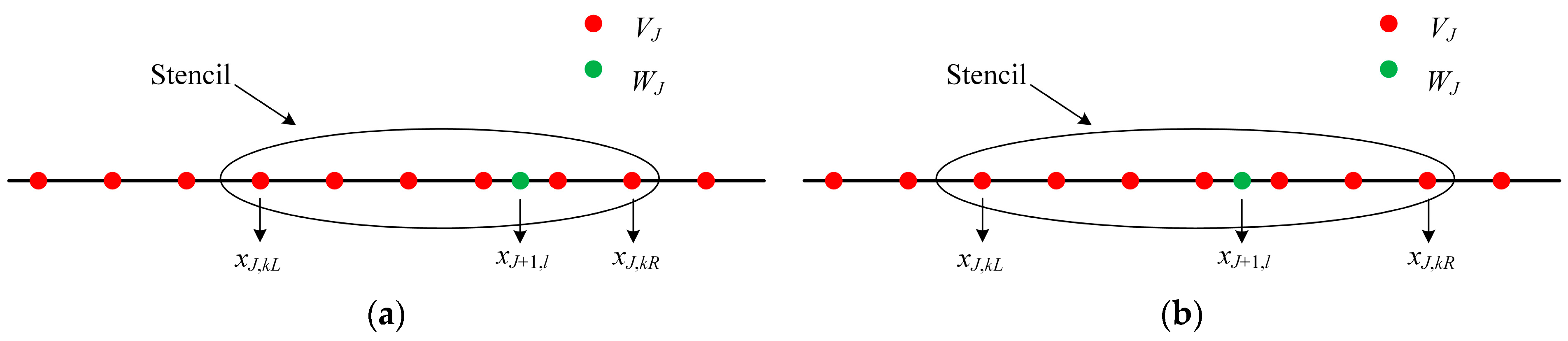
For convenience of discussion, we define two parameters to depict asymmetrical properties. We take scaling functions with N = 6 and N = 7 as examples. The stencils for the scaling functions are shown in Figure 1. The bias magnitude of the stencil is defined by the difference between the number of nodes on the left side of and that on the right side of as denoted by the BM. To evaluate the symmetry of the scaling functions, we also use symmetry factor (SF) to evaluate the symmetry of the scaling functions, which can be calculated by
where IL is the length of the support interval on the left side of the zero point, and IR is the length of the support interval on the right side of the zero point. The scaling function is exactly symmetrical when SF = 1. We can provide an explicit formula to compute the SF base on the BM as follows:
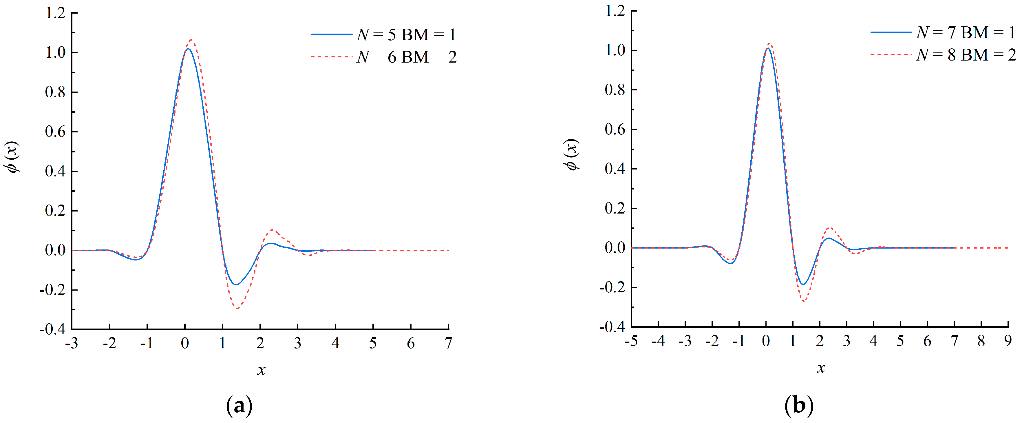
It can be observed from Equation (18) that the SF approaches to 1 as N tends to infinity, which reveals that the symmetry of the scaling function is improved as N increases. For a specified N, the SF decreases with an increment in BM. The BM and SF of the scaling functions used in the present paper for analyzing the stability and resolution of the wavelet upwind schemes are listed in Table 1. We note that the BM has the same parity with the N. The SF with the Nodd is greater than that with the Neven when the BModd and Nodd are both smaller than the BMeven and Neven by one, respectively. Here, the subscript represents the parity of the N. Some scaling functions are shown in Figure 2 as examples.
3. Stability and Resolution Analysis of Wavelet Upwind Schemes
In this section, we conduct two benchmark tests by applying different schemes from N = 3 to N = 10. Two kinds of norms are defined to evaluate numerical errors, as follows:
where is the exact solution and is the numerical one.
Numerical examples are performed to the following one-dimensional linear scalar equation:
where a = 1.
3.1. Advection of a Sine Wave
At first, we verify orders of accuracy and explore the stability of the proposed schemes by refinement tests. A sine wave as the initial condition is presented as follows:
The periodic boundary condition is addressed based on the extension method for periodic functions proposed in our previous work [37].
The numerical errors are calculated at t = 2. BModd = 1 and BMeven = 2 are taken for the different schemes. The time steps are set small enough to remove the influence of time integration. The numerical errors and orders of accuracy for all schemes are shown in Table 2. It should be noted that errors which are smaller than are removed from the table since they approach the machine precision of the double type. Theorem 2 shows that the theoretical order of accuracy of the scheme is (N – 1) order. It can be seen that the orders of accuracy are consistent with the expected ones for the schemes where N is smaller than 8. Higher order schemes give the expected orders of accuracy when the number of nodes is small. The N = 4 scheme is unstable even for this smooth wave evolution in our tests. Therefore, the result is absent from Table 2.
To explore the effects of the asymmetry of the scaling function on stability, we also compute the numerical results by, respectively, using the wavelet schemes with N = 7, N = 9, and different BM values, as shown in Table 3. It can be observed that the scheme with N = 7 and BM = 3 is unstable because the error increases significantly as J goes up to 8. We conclude that the scheme with the same N will be unstable when the asymmetry of the scaling function increases.
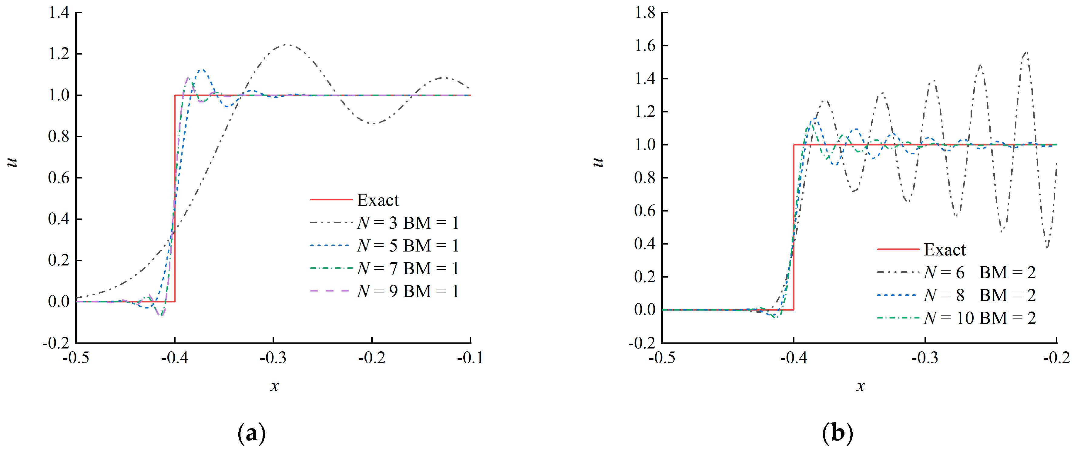
3.2. Advection of a Square Wave
To validate the stability of the schemes to solve a jump discontinuity problem, we conduct the advection of a square wave, which has the following initial distribution:
The Fourier series of the square wave is the infinite superposition of sine and cosine waves, and contains all frequency components. Numerical results at t = 8 obtained by different wavelet schemes at the resolution level J = 8 are illustrated in Figure 3. It can be seen that spurious oscillations pollute numerical solutions near the jump discontinuities for almost all schemes. Figure 3b shows that the oscillations obtained by the scheme with N = 6 are gradually amplified in the positive direction, which indicates that the scheme is unstable for discontinuity problems. For all the schemes with a specified parity of N, the length of the oscillation interval decreases with an increment in N. We continue to compute the results at t = 32, as shown in Figure 4. The results for the scheme with N = 6 are divergent for long-term time integration, which is not depicted in the figure. Although this scheme is stable for the single sine wave advection, it behaves unstably for that of the waves with multiple or infinite frequencies. It can be observed that the schemes with N ∈ odd confine spurious oscillations to the thinner region, and the amplitude of the oscillations attenuates rapidly. In addition, N = 7, BM = 3 and N = 9, BM = 3 schemes are unstable for the current problem.
3.3. Dissipation and Dispersion Analysis
Although we can devise wavelet upwind schemes based on our proposed method, the above numerical tests suggest that some of the wavelet schemes are unstable even for the linear scalar advection problems. Therefore, it is crucial to investigate the dissipation and dispersion properties and provide an instruction to choose “good” wavelets for stable wavelet upwind schemes.
We examine the dissipation and dispersion properties of the schemes based on the Fourier analysis method [2,30]. Suppose that , then we can obtain the numerical derivative:
where is the corrected wavenumber, which is a complex variable, and . Therefore, can be rewritten as . The exact derivative is given by
Comparing the above relation, we can find that kr = 0 and ki = kΔx for ideal numerical schemes. When conducting Fourier analysis on Equation (21), we can calculate the following numerical solution:
where kr is the dissipation coefficient and ki is the dispersion coefficient. The exact solution for Equation (21) can be computed by
Then, we can give the physical meaning of kr and ki. kr depicts the attenuation of the wave amplitude at t induced by the numerical error, and ki describes the change in propagation speed of the wave caused by the numerical method. It can be noted that the wave amplitude will be amplified over time if kr is a negative value. The corresponding scheme shows the instability when solving the advection problems. Therefore, kr for stable numerical schemes should be non-negative. Here, kΔx is defined as an effective wavenumber and denoted by α. When ki/α > 1, the numerical wave will run faster than the exact one. Additionally, the numerical wave will fall behind the exact wave for ki/α < 1. We remark that only the spectral method has the ideal dispersion property, which means that ki/α = 1.
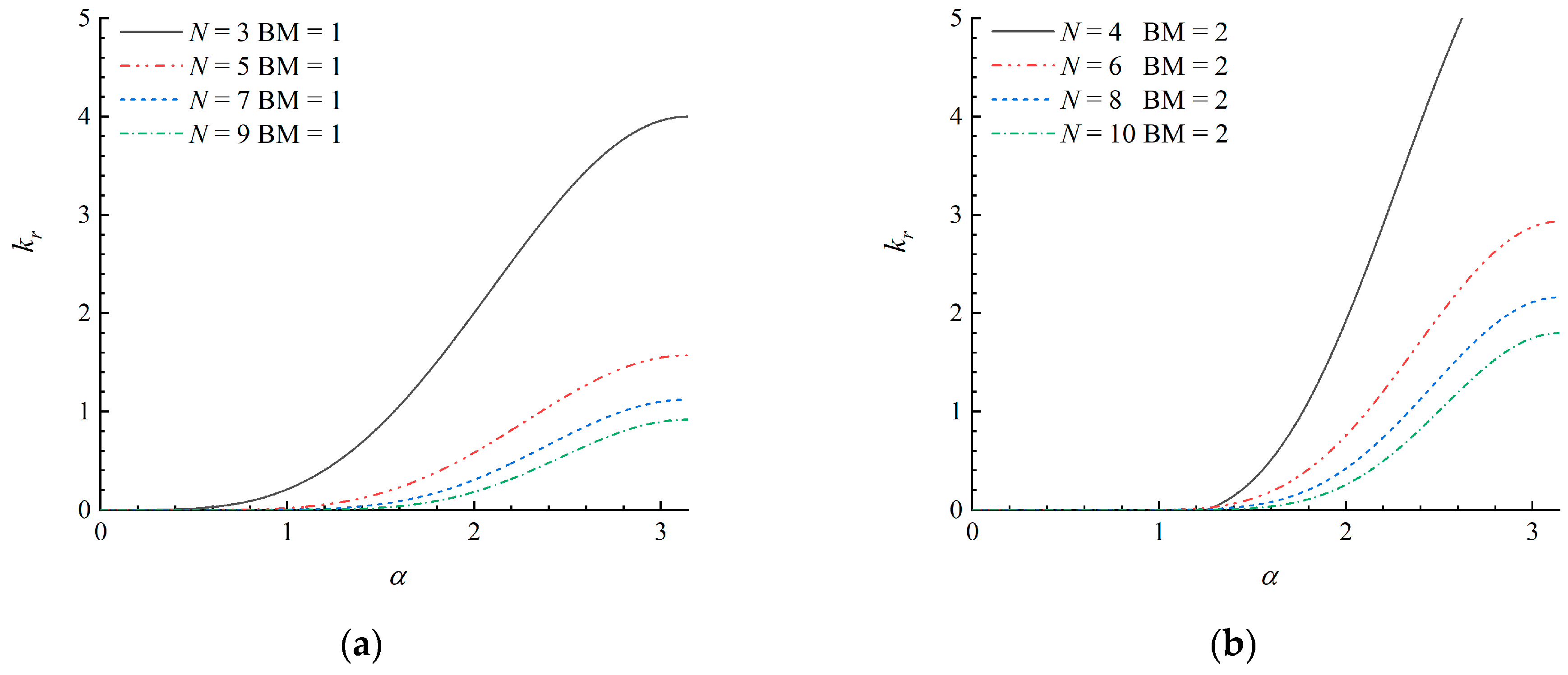
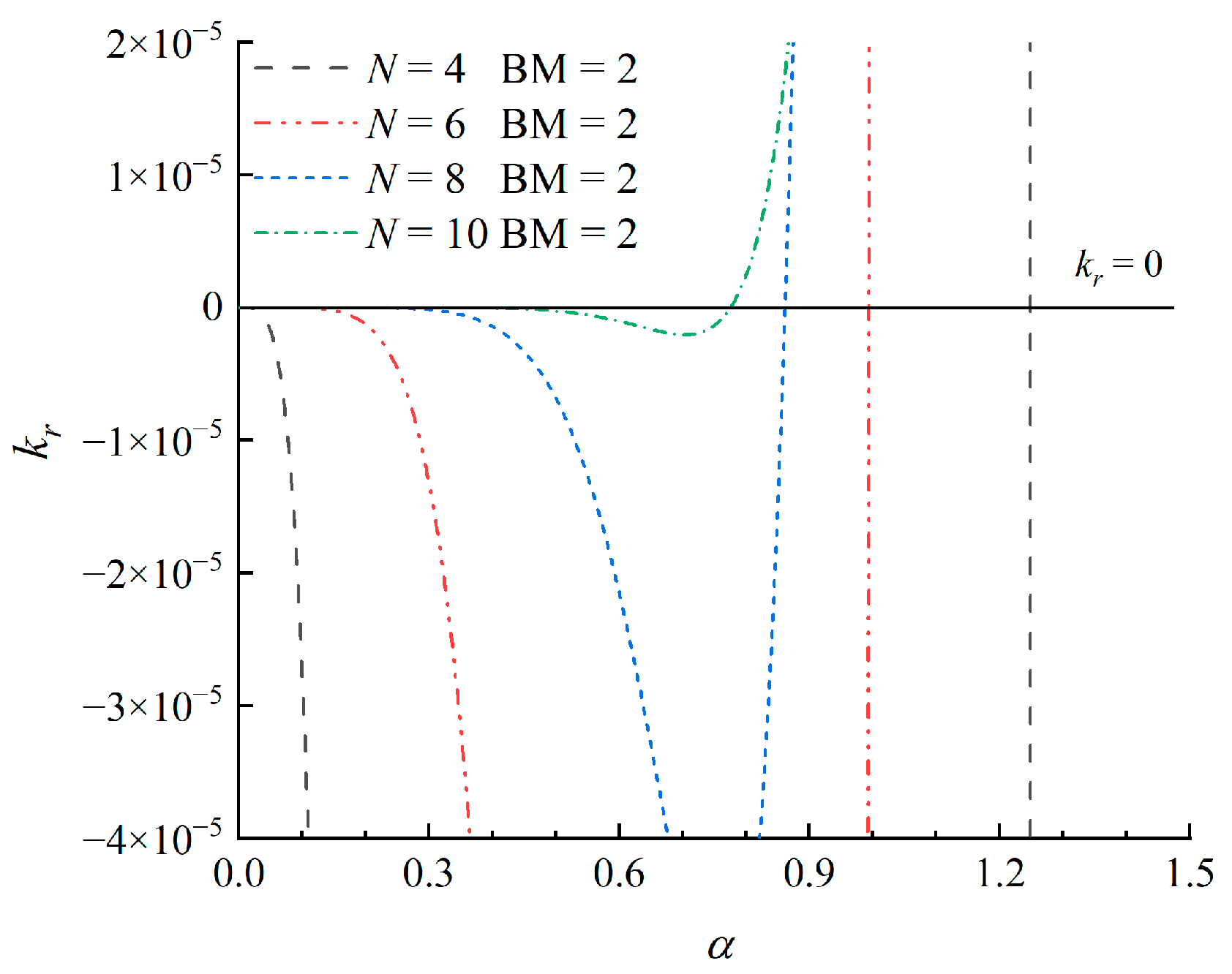
We compute the dissipation coefficient of the different wavelet schemes as shown in Figure 5. For a specified parity of N, it can be seen that kr decreases with an increase of N. The kr of the scheme with N ∈ odd is smaller than that with N ∈ even, indicating that the wavelet upwind schemes with N ∈ odd show better dissipation property. To seek the reason for the instability of several schemes, we analyze the kr for all the above schemes. We find that the negative kr exists for schemes with N ∈ even. To clarify this fact, the locally enlarged version of Figure 5b is illustrated in Figure 6. It can be observed that kr are all negative when α < 0.8. This suggests that the schemes with N ∈ even will show a negative diffusion phenomenon when J is large enough, and the error will be amplified over time. This actually induces the instability of the wavelet schemes. We also find that the local extreme value approaches to 0 as N increases for N ∈ even, which means that the negative diffusion process is weakened and the stability of the schemes is improved. This explains how the numerical tests for the schemes with N ∈ even in Section 3.1 and Section 3.2 are still stable. However, for longer time integration and some α near the local extreme value, the results might be divergent. In addition, the reason that the scheme with N = 4, BM = 2 is unstable for the sine wave evolution can also be uncovered based on the dissipation analysis. It can be observed that the scheme with N = 4, BM = 2 has the largest negative dissipation zone of the effective wavenumber α among all the candidates of the wavelet schemes caused by the severest asymmetry, leading to the instability for solving the smooth wave evolution even with far fewer nodes.
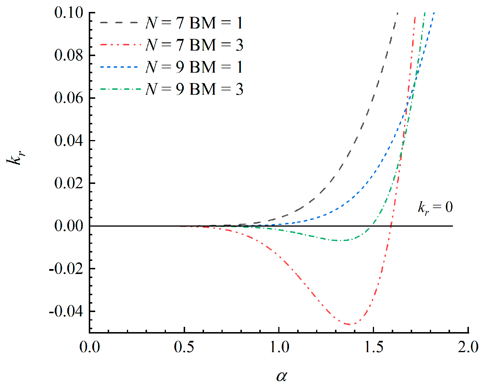
Based on the above analysis, we can conclude that only N ∈ odd schemes provide the correct implicit viscosity for solving the hyperbolic conservation laws. However, numerical tests in Section 3.1 show that the scheme with N = 7 and BM = 3 is still unstable. As has been discussed, the asymmetry of the scaling function is another factor influencing the stability of the wavelet schemes. We further evaluate the dissipation coefficients of the schemes with N = 7, BM = 3 and N = 9, BM = 3 as shown in Figure 7. It can be found that kr is negative when α is smaller than the specified value. Therefore, the schemes with BM = 3 are unstable. Now, we can achieve a basic instruction that N ∈ odd, BM = 1 schemes have non-negative dissipation coefficients and are stable for hyperbolic conservation laws.
Then, we will explore the dispersion property related to the resolution of the schemes. For a specified wavelet scheme, an effective node number is defined by the point per wavelength, abbreviated as PPW, which can be computed by the following relation:
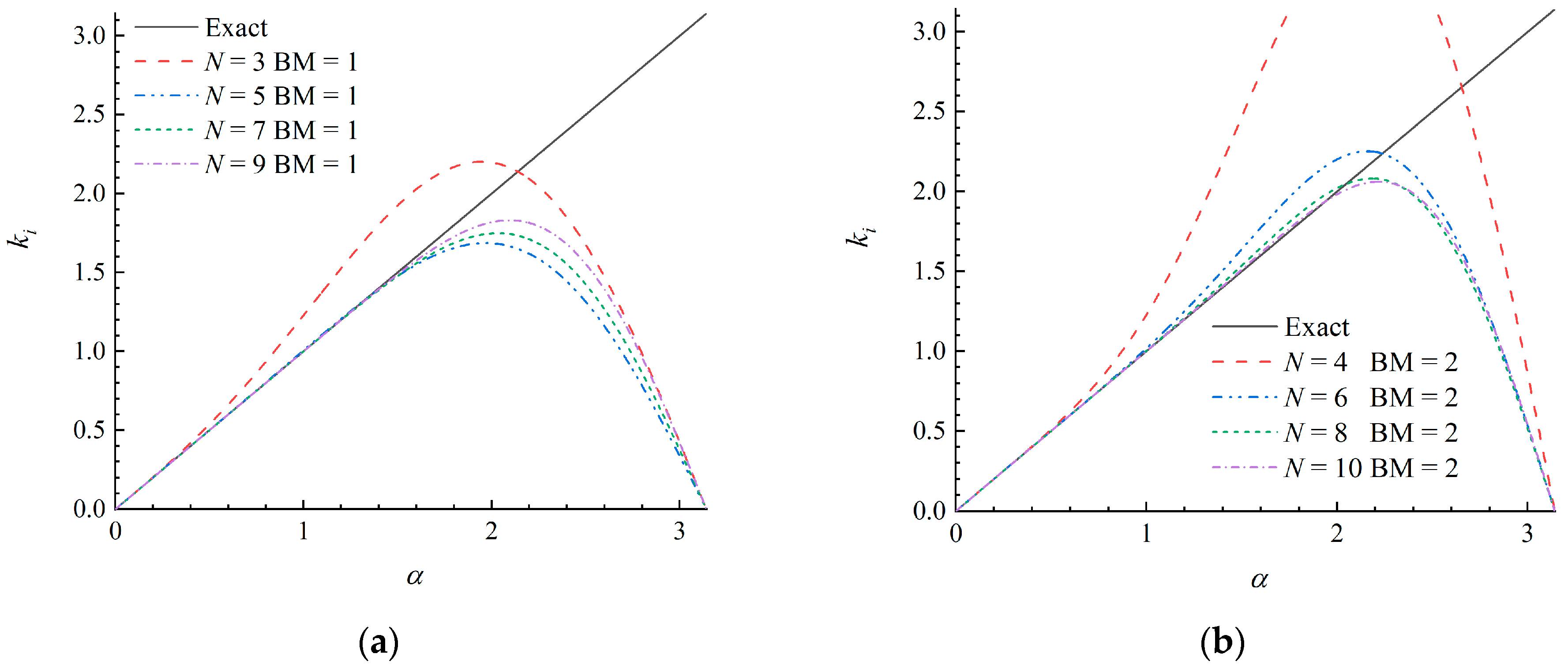
The spectral method has the optimal resolution corresponding to α = π and PPW = 2. It can be seen from Equation (28) that PPW is inversely proportional to α. The length of the interval α that ki / α is approximately equal to 1 depicts the ability of the scheme to trace the wave accurately. We choose the interval of α that satisfies and to measure the maximum α, which reflects the resolution of the schemes directly. The dispersion coefficients against α are plotted in Figure 8. It can be observed that N < 5 schemes have a large dispersion error and a low resolution. The maximum α where ki/α meets the tolerance relation increases with an increment in N for the specified parity. To clarify the resolution more clearly, we list the maximum α in the tolerance range in Table 4. It can be seen that the maximum α gradually tends to π as N increases, and the schemes with N ∈ even behave better in resolution when N > 6. On the basis of the above analysis, we can find that the wavelets are more applicable to design the high-order schemes, and the scheme with larger N has the higher accuracy and better resolution.
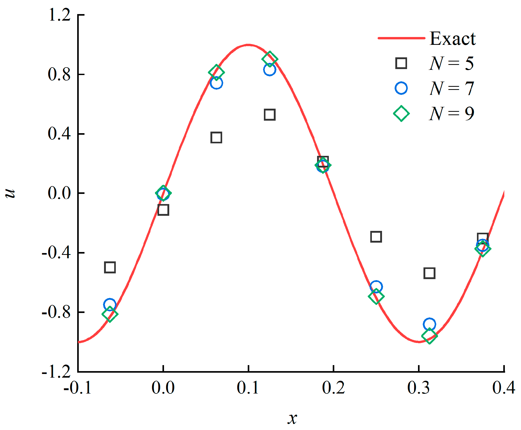
Next, we conduct a numerical test with a smooth initial distribution to verify the theoretical analysis of the dissipation and dispersion performance. The test is the advection of a sine wave described in Section 3.1 with u (x, 0) = sin (5πx) as the initial condition. The PPW is approximately equal to 6 at the resolution level J = 4. The numerical results obtained by the schemes with N ∈ odd and BM = 1 at t = 2 are shown in Figure 9. It can be seen that the higher order schemes show themselves to be less dissipative, approach the exact solution more accurately and reveal a higher resolution for the wave. Therefore, the numerical results are in accordance with the stability and resolution analysis.
Finally, a numerical test of the advection of a multi-scale function is devised to show the capability of the wavelet schemes in recognizing smooth and discontinuous solutions in the high-speed flows. The initial condition consists of step functions, saw-tooth function and sine waves in different frequencies, which is shown as:
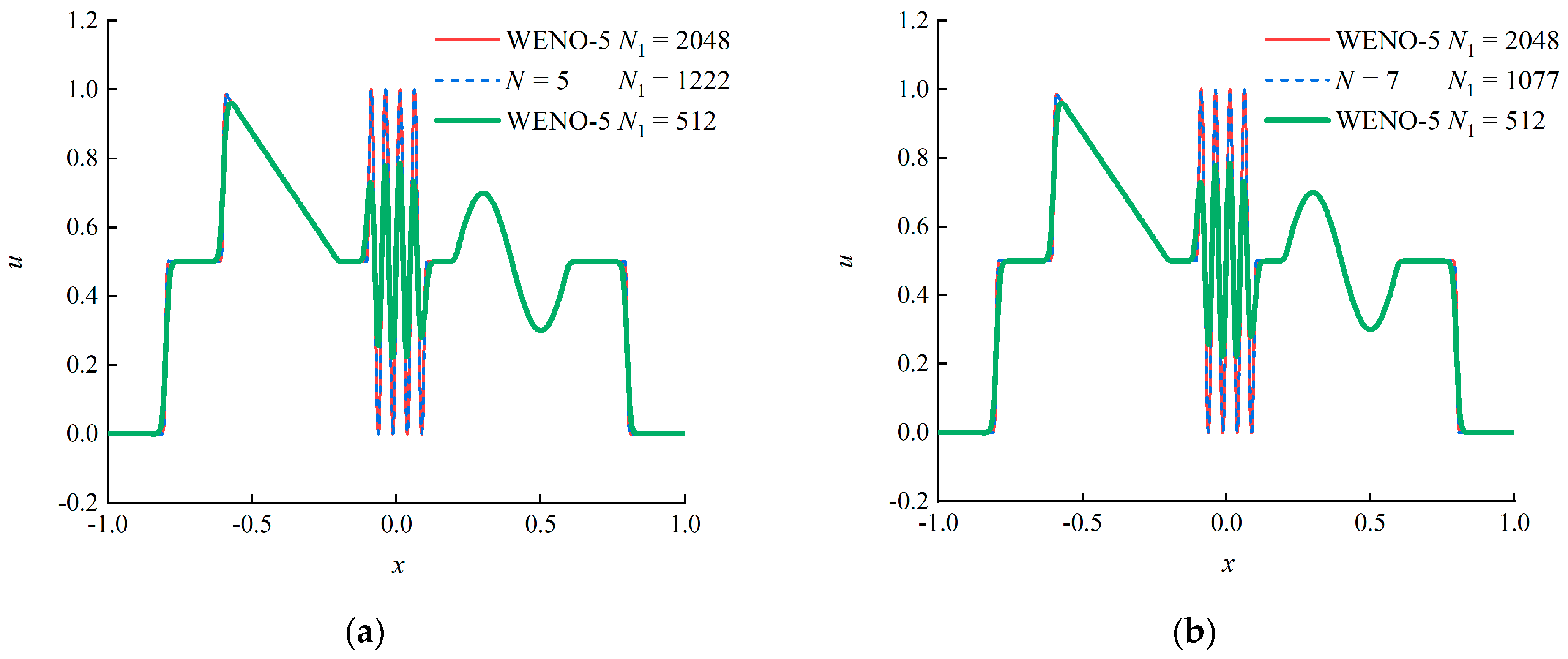
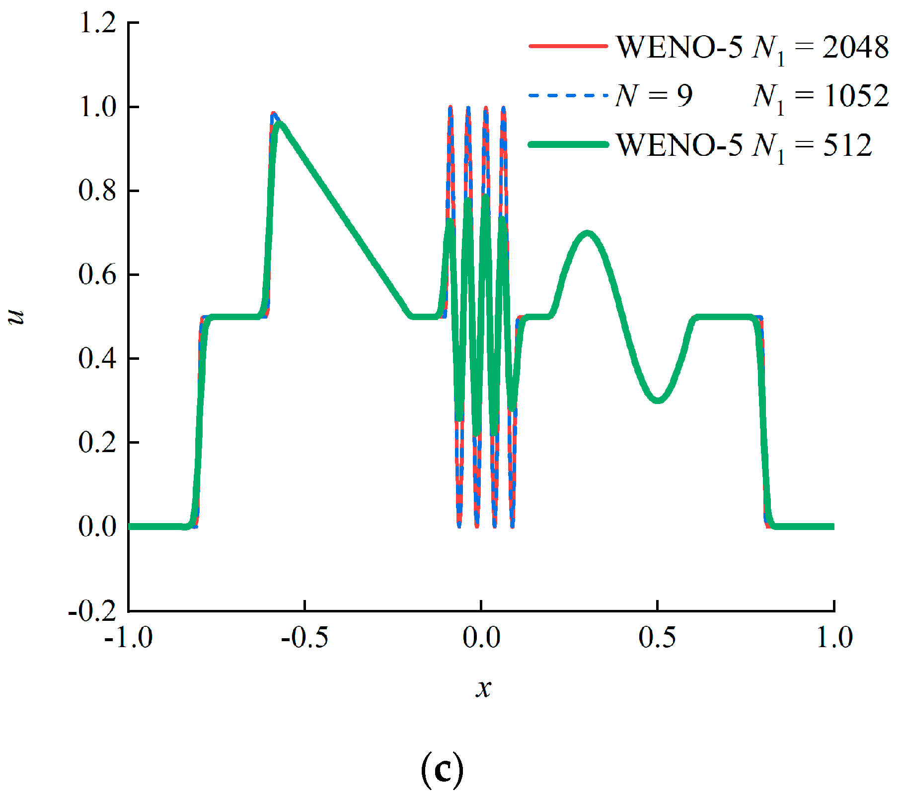
For this numerical test, we apply the adaptive wavelet upwind schemes proposed in our previous study [28]. The main idea of adaptive node generation is to recognize trouble nodes based on the wavelet coefficients that are larger than a threshold parameter ε = 10−5, and insert nodes in the adjacent zones near the trouble nodes. Moreover, an integration reconstruction method is designed based on the Lebesgue differentiation theorem to suppress the spurious oscillations. We choose the basic resolution level J0 = 6, the maximum resolution level Jmax = 12, and the same adaptive and reconstruction parameters for different schemes. The numerical results obtained by the adaptive wavelet schemes with N ∈ odd and BM = 1 at t = 2 are compared with that of the classic fifth-order finite difference WENO scheme (WENO-5) proposed by Jiang and Shu [38], as illustrated in Figure 10. It can be found that the higher order wavelet schemes can capture the discontinuities without spurious oscillations and distinguish different scale structures accurately with fewer nodes, which also verifies the better resolution of the higher order schemes. For the WENO-5 scheme, a uniform node distribution with N1 = 2048 is required to depict all the details of the solution. The nodes required in the adaptive wavelet upwind schemes are about half of the WENO-5 scheme, showing that the adaptive wavelet schemes with the integration reconstruction can capture discontinuities free from the numerical oscillations and distinguish complex solutions efficiently.
4. Conclusions
In the present paper, we constructed a system of wavelet collocation upwind schemes and conducted linear advection tests and Fourier analysis to uncover the effects of the characteristics of scaling functions on the stability and resolution of the constructed schemes. The convergence rates of the schemes were consistent with our expectations. The dissipation analysis suggested that one can apply scaling functions of the wavelets with N ∈ odd, BM = 1 to construct the high-order and stable upwind schemes for hyperbolic conservation laws. The higher order scheme had a better resolution, which tended to the spectral resolution as N increased. Two typical numerical tests verified that the constructed wavelet collocation upwind schemes had the desired properties and can be used to solve high-speed flows with multi-scale smooth structures and discontinuities in an efficient way.
Author Contributions
Conceptualization, J.W.; methodology, J.W. and B.Y.; writing—original draft preparation, B.Y.; writing—review and editing, X.L. and J.W.; supervision, J.W. and Y.Z. All authors have read and agreed to the published version of the manuscript.
Funding
This research was supported by grants from the National Natural Science Foundation of China (11925204).
Data Availability Statement
Data are available on request due to restrictions of privacy.
Conflicts of Interest
The authors declare no conflict of interest.
Appendix A
The auto correlation of Daubechies scaling functions [33,39] and the interpolation method [40] are the main techniques to devise scaling functions of interpolation wavelets. The interpolation method provides more freedom to construct symmetric and asymmetric scaling functions. Therefore, we apply the interpolation method to devise the scaling functions of the interpolation wavelets. The procedure of building positive upwind wavelets is elaborated as follows:
First, we choose the smoothness parameter N. For an asymmetrical wavelet, N ∈ even or N ∈ odd is optional.
Second, we select the BM and the node stencil. Specify N nodes uniformly distributed in VJ as the base and locate one node in WJ. The BM has the same parity with N. Several candidates are allowed for the positive upwind wavelets with BM > 0.
Third, we approximate by the (N − 1)th order Lagrange interpolation polynomial and calculate the filter coefficients. The following relation is derived:
where and . On the basis of the refinement relation,
Substituting (A2) into (A1), hl = δ0,l can be easily calculated when l ∈ even. For l ∈ odd, hl can be computed by
To compute the coefficients more efficiently, supposing that J = 0 and k = 0 can obtain
Finally, we calculate the derivatives and integrals of the scaling function by algorithms proposed by Wang [41] and Chen et al. [42]. Applying the refinement relation and the cascade algorithm, the values of the scaling function, its derivatives and integrals at dyadic points at arbitrary refined resolution levels can be obtained.
The filter coefficients of the negative upwind wavelets are of mirror symmetry with those of the corresponding positive upwind wavelets. Following the above steps, a desirable scaling function can be built. For the interpolation method, the Kronecker delta function is chosen as the dual scaling function [40]:
Finally, the idea proposed by Donoho [39], which constructs a wavelet function from the scaling function, is followed:
References
- Pirozzoli, S. Numerical Methods for High-Speed Flows. Annu. Rev. Fluid Mech. 2011, 43, 163–194. [Google Scholar] [CrossRef]
- Lele, S.K. Compact finite difference schemes with spectral-like resolution. J. Comput. Phys. 1992, 103, 16–42. [Google Scholar] [CrossRef]
- Kurganov, A.; Tadmor, E. New High-Resolution Central Schemes for Nonlinear Conservation Laws and Convection–Diffusion Equations. J. Comput. Phys. 2000, 160, 241–282. [Google Scholar] [CrossRef]
- Roe, P.L. Characteristic-Based Schemes for the Euler Equations. Annu. Rev. Fluid Mech. 1986, 18, 337–365. [Google Scholar] [CrossRef]
- Moretti, G. The λ-scheme. Comput. Fluids 1979, 7, 191–205. [Google Scholar] [CrossRef]
- Regele, J.D.; Vasilyev, O.V. An adaptive wavelet-collocation method for shock computations. Int. J. Comput. Fluid Dyn. 2009, 23, 503–518. [Google Scholar] [CrossRef]
- Shu, C.-W. High order WENO and DG methods for time-dependent convection-dominated PDEs: A brief survey of several recent developments. J. Comput. Phys. 2016, 316, 598–613. [Google Scholar] [CrossRef]
- Harten, A.; Engquist, B.; Osher, S.; Chakravarthy, S.R. Uniformly high order accurate essentially non-oscillatory schemes, III. J. Comput. Phys. 1987, 71, 231–303. [Google Scholar] [CrossRef]
- Liu, X.D.; Osher, S.; Chan, T. Weighted Essentially Non-oscillatory Schemes. J. Comput. Phys. 1994, 115, 200–212. [Google Scholar] [CrossRef]
- Ii, S.; Xiao, F. High order multi-moment constrained finite volume method. Part I: Basic formulation. J. Comput. Phys. 2009, 228, 3669–3707. [Google Scholar] [CrossRef] [Green Version]
- Cockburn, B.; Shu, C.-W. TVB Runge-Kutta Local Projection Discontinuous Galerkin Finite Element Method for Conservation Laws II: General Framework. Math. Comput. 1989, 52, 411–435. [Google Scholar]
- Hughes, T.J.R.; Mallet, M.; Akira, M. A new finite element formulation for computational fluid dynamics: II. Beyond SUPG. Comput. Methods Appl. Mech. Eng. 1986, 54, 341–355. [Google Scholar] [CrossRef]
- Schneider, K.; Vasilyev, O.V. Wavelet methods in computational fluid dynamics. Annu. Rev. Fluid Mech. 2010, 42, 473–503. [Google Scholar] [CrossRef]
- Vasilyev, O.V.; Paolucci, S. A Dynamically Adaptive Multilevel Wavelet Collocation Method for Solving Partial Differential Equations in a Finite Domain. J. Comput. Phys. 1996, 125, 498–512. [Google Scholar] [CrossRef]
- Vasilyev, O.V. Solving Multi-dimensional Evolution Problems with Localized Structures using Second Generation Wavelets. Int. J. Comput. Fluid Dyn. 2003, 17, 151–168. [Google Scholar] [CrossRef]
- De Stefano, G.; Vasilyev, O.V. A fully adaptive wavelet-based approach to homogeneous turbulence simulation. J. Fluid Mech. 2012, 695, 149–172. [Google Scholar] [CrossRef]
- De Stefano, G.; Brown-Dymkoski, E.; Vasilyev, O.V. Wavelet-based adaptive large-eddy simulation of supersonic channel flow. J. Fluid Mech. 2020, 901, A13. [Google Scholar] [CrossRef]
- Chaurasiya, V.; Kumar, D.; Rai, K.N.; Singh, J. A computational solution of a phase-change material in the presence of convection under the most generalized boundary condition. Therm. Sci. Eng. Prog. 2020, 20, 100664. [Google Scholar] [CrossRef]
- Jitendra; Chaurasiya, V.; Rai, K.N.; Singh, J. Legendre wavelet residual approach for moving boundary problem with variable thermal physical properties. Int. J. Nonlinear Sci. Numer. Simul. 2022, 23, 957–970. [Google Scholar] [CrossRef]
- Engels, T.; Schneider, K.; Reiss, J.; Farge, M. A Wavelet-Adaptive Method for Multiscale Simulation of Turbulent Flows in Flying Insects. Commun. Comput. Phys. 2021, 30, 1118–1149. [Google Scholar]
- Vuik, M.J.; Ryan, J.K. Multiwavelet troubled-cell indicator for discontinuity detection of discontinuous Galerkin schemes. J. Comput. Phys. 2014, 270, 138–160. [Google Scholar] [CrossRef]
- Do, S.; Li, H.; Kang, M. Wavelet-based adaptation methodology combined with finite difference WENO to solve ideal magnetohydrodynamics. J. Comput. Phys. 2017, 339, 482–499. [Google Scholar] [CrossRef]
- Restrepo, J.M.; Leaf, G.K. Wavelet-Galerkin Discretization of Hyperbolic Equations. J. Comput. Phys. 1995, 122, 118–128. [Google Scholar] [CrossRef]
- Hughes, T.J.R.; Franca, L.P.; Mallet, M. A new finite element formulation for computational fluid dynamics: I. Symmetric forms of the compressible Euler and Navier-Stokes equations and the second law of thermodynamics. Comput. Methods Appl. Mech. Eng. 1986, 54, 223–234. [Google Scholar] [CrossRef]
- Pereira, R.M.; Nguyen Van Yen, N.; Schneider, K.; Farge, M. Adaptive Solution of Initial Value Problems by a Dynamical Galerkin Scheme. Multiscale Model. Simul. 2022, 20, 1147–1166. [Google Scholar] [CrossRef]
- Bertoluzza, S. Adaptive wavelet collocation method for the solution of Burgers equation. Transp. Theory Stat. Phys. 1996, 25, 339–352. [Google Scholar] [CrossRef]
- Alam, J.M.; Kevlahan, N.K.-R.; Vasilyev, O.V. Simultaneous space–time adaptive wavelet solution of nonlinear parabolic differential equations. J. Comput. Phys. 2006, 214, 829–857. [Google Scholar] [CrossRef]
- Yang, B.; Wang, J.; Liu, X.; Zhou, Y. High-order adaptive multiresolution wavelet upwind schemes for hyperbolic conservation laws. arXiv 2023, arXiv:2301.01090. [Google Scholar]
- Warming, R.F.; Hyett, B.J. The modified equation approach to the stability and accuracy analysis of finite-difference methods. J. Comput. Phys. 1974, 14, 159–179. [Google Scholar] [CrossRef]
- Vichnevetsky, R.; Bowles, J.B. Fourier Analysis of Numerical Approximations of Hyperbolic Equations, 2nd ed.; Society for Industrial and Applied Mathematics: Philadelphi, PA, USA, 1982. [Google Scholar]
- Pirozzoli, S. On the spectral properties of shock-capturing schemes. J. Comput. Phys. 2006, 219, 489–497. [Google Scholar] [CrossRef]
- Ciarlet, P.G. Linear and Nonlinear Functional Analysis with Applications; Society for Industrial and Applied Mathematics: Philadelphia, PA, USA, 2013. [Google Scholar]
- Liu, X.; Liu, G.; Wang, J.; Zhou, Y. A wavelet multiresolution interpolation Galerkin method for targeted local solution enrichment. Comput. Mech 2019, 64, 989–1016. [Google Scholar] [CrossRef]
- Liu, X.; Liu, G.R.; Wang, J.; Zhou, Y. A wavelet multi-resolution enabled interpolation Galerkin method for two-dimensional solids. Eng. Anal. Bound. Elem. 2020, 117, 251–268. [Google Scholar] [CrossRef]
- Zhang, L.; Wang, J.; Liu, X.; Zhou, Y. A wavelet integral collocation method for nonlinear boundary value problems in physics. Comput. Phys. Commun. 2017, 215, 91–102. [Google Scholar] [CrossRef] [Green Version]
- Beylkin, G.; Keiser, J.M. On the Adaptive Numerical Solution of Nonlinear Partial Differential Equations in Wavelet Bases. J. Comput. Phys. 1997, 132, 233–259. [Google Scholar] [CrossRef]
- Liu, X.; Zhou, Y.; Wang, J. A space-time fully decoupled wavelet Galerkin method for solving two-dimensional Burgers’ equations. Comput. Math. Appl. 2016, 72, 2908–2919. [Google Scholar] [CrossRef]
- Jiang, G.-S.; Shu, C.-W. Efficient Implementation of Weighted ENO Schemes. J. Comput. Phys. 1996, 126, 202–228. [Google Scholar] [CrossRef]
- Donoho, D.L. Interpolating wavelet transforms. Prepr. Dep. Stat. Stanf. Univ. 1992, 2, 1–54. [Google Scholar]
- Sweldens, W.; Schroder, P. Building Your Own Wavelets at Home; Springer: Berlin/Heidelberg, Germany, 2005. [Google Scholar]
- Wang, J. Generalized Theory and Arithmetic of Orthogonal Wavelets and Applications to Researches of Mechanics Including Piezoelectric Smart Structures. Ph.D Thesis, Lanzhou University, Lanzhou, China, 2001. [Google Scholar]
- Chen, M.-Q.; Hwang, C.; Shih, Y.-P. The computation of wavelet-Galerkin approximation on a bounded interval. Int. J. Numer. Methods Eng. 1996, 39, 2921–2944. [Google Scholar] [CrossRef]
Figure 1.
Examples of stencils: (a) Stencil for the asymmetrical wavelet with N = 6 and BM = 2; (b) Stencil for the asymmetrical wavelet with N = 7 and BM = 1.
Figure 1.
Examples of stencils: (a) Stencil for the asymmetrical wavelet with N = 6 and BM = 2; (b) Stencil for the asymmetrical wavelet with N = 7 and BM = 1.

Figure 2.
Examples of some asymmetrical scaling functions: (a) Scaling functions with N = 5 and N = 6; (b) Scaling functions with N = 7 and N = 8.
Figure 2.
Examples of some asymmetrical scaling functions: (a) Scaling functions with N = 5 and N = 6; (b) Scaling functions with N = 7 and N = 8.

Figure 3.
Advection of a square wave by the different schemes at t = 8, J = 8: (a) N ∈ odd; (b) N ∈ even.
Figure 3.
Advection of a square wave by the different schemes at t = 8, J = 8: (a) N ∈ odd; (b) N ∈ even.

Figure 4.
Advection of a square wave by the different schemes at t = 32, J = 8: (a) N ∈ odd; (b) N ∈ even.
Figure 4.
Advection of a square wave by the different schemes at t = 32, J = 8: (a) N ∈ odd; (b) N ∈ even.

Figure 5.
Dissipation analysis of the different wavelet schemes: (a) N ∈ odd; (b) N ∈ even.

Figure 6.
Locally enlarged version of the dissipation analysis of N ∈ even schemes.

Figure 7.
Comparison of dissipation coefficients of N = 7 and N = 9 schemes.

Figure 8.
Dispersion coefficients against α in different wavelet schemes: (a) N ∈ odd; (b) N ∈ even.
Figure 8.
Dispersion coefficients against α in different wavelet schemes: (a) N ∈ odd; (b) N ∈ even.

Figure 9.
Numerical results by the schemes with N ∈ odd and BM = 1 at t = 2, J = 4.

Figure 10.
Numerical results by the schemes with N ∈ odd and BM = 1 at t = 2 (J0 = 6, Jmax = 12): (a) N = 5; (b) N = 7; (c) N = 9.
Figure 10.
Numerical results by the schemes with N ∈ odd and BM = 1 at t = 2 (J0 = 6, Jmax = 12): (a) N = 5; (b) N = 7; (c) N = 9.


Table 1.
BM and SF for the scaling functions.
| N | 3 | 4 | 5 | 6 | 7 | 7 | 8 | 9 | 9 | 10 |
|---|---|---|---|---|---|---|---|---|---|---|
| BM | 1 | 2 | 1 | 2 | 1 | 3 | 2 | 1 | 3 | 2 |
| SF | 0.33 | 0.20 | 0.60 | 0.43 | 0.71 | 0.33 | 0.56 | 0.78 | 0.45 | 0.64 |
Table 2.
Numerical results for the sine wave advection.
| Method | N1 | l∞ Error | l∞ Order | l2 Error | l2 Order |
|---|---|---|---|---|---|
| N = 3 (2nd order) | 32 | 8.00 × 10⁻² | — | 8.24 × 10⁻² | — |
| 64 | 2.02 × 10⁻² | 1.99 | 2.05 × 10⁻² | 2.01 | |
| 128 | 5.05 × 10⁻³ | 2.00 | 5.08 × 10⁻³ | 2.01 | |
| 256 | 1.26 × 10⁻³ | 2.00 | 1.27 × 10⁻³ | 2.01 | |
| 512 | 3.15 × 10⁻⁴ | 2.00 | 3.16 × 10⁻⁴ | 2.00 | |
| N = 5 (4th order) | 32 | 1.84 × 10⁻⁴ | — | 1.90 × 10⁻⁴ | — |
| 64 | 1.15 × 10⁻⁵ | 4.01 | 1.16 × 10⁻⁵ | 4.03 | |
| 128 | 7.15 × 10⁻⁷ | 4.00 | 7.21 × 10⁻⁷ | 4.01 | |
| 256 | 4.47 × 10⁻⁸ | 4.00 | 4.49 × 10⁻⁸ | 4.01 | |
| 512 | 2.79 × 10⁻⁹ | 4.00 | 2.80 × 10⁻⁹ | 4.00 | |
| N = 6 (5th order) | 32 | 3.78 × 10⁻⁵ | — | 3.80 × 10⁻⁵ | — |
| 64 | 1.18 × 10⁻⁶ | 4.99 | 1.19 × 10⁻⁶ | 5.00 | |
| 128 | 3.71 × 10⁻⁸ | 5.00 | 3.71 × 10⁻⁸ | 5.00 | |
| 256 | 1.16 × 10⁻⁹ | 5.00 | 1.16 × 10⁻⁹ | 5.00 | |
| 512 | 3.64 × 10⁻¹¹ | 4.99 | 3.64 × 10⁻¹¹ | 4.99 | |
| N = 7 (6th order) | 32 | 1.02 × 10⁻⁶ | — | 1.04 × 10⁻⁶ | — |
| 64 | 1.46 × 10⁻⁸ | 6.12 | 1.48 × 10⁻⁸ | 6.14 | |
| 128 | 1.71 × 10⁻¹⁰ | 6.42 | 1.73 × 10⁻¹⁰ | 6.42 | |
| 256 | 8.70 × 10⁻¹³ | 7.61 | 8.75 × 10⁻¹³ | 7.62 | |
| N = 8 (7th order) | 32 | 2.12 × 10⁻⁷ | — | 2.13 × 10⁻⁷ | — |
| 64 | 1.64 × 10⁻⁹ | 7.01 | 1.64 × 10⁻⁹ | 7.02 | |
| 128 | 1.33 × 10⁻¹¹ | 6.95 | 1.33 × 10⁻¹¹ | 6.95 | |
| N = 9 (8th order) | 32 | 7.18 × 10⁻⁹ | — | 7.38 × 10⁻⁹ | — |
| 64 | 2.27 × 10⁻¹¹ | 8.31 | 2.30 × 10⁻¹¹ | 8.33 | |
| N = 10 (9th order) | 32 | 1.45 × 10⁻⁹ | — | 1.46 × 10⁻⁹ | — |
| 64 | 2.77 × 10⁻¹² | 9.03 | 2.77 × 10⁻¹² | 9.04 |
Table 3.
Numerical errors and order of accuracy for one-dimensional linear scalar equation.
| Method | N1 | l∞ Error | l∞ Order | l2 Error | l2 Order |
|---|---|---|---|---|---|
| N = 7 BM = 1 (6th order) | 32 | 1.02 × 10⁻⁶ | — | 1.04 × 10⁻⁶ | — |
| 64 | 1.46 × 10⁻⁸ | 6.12 | 1.48 × 10⁻⁸ | 6.14 | |
| 128 | 1.71 × 10⁻¹⁰ | 6.42 | 1.73 × 10⁻¹⁰ | 6.42 | |
| 256 | 8.70 × 10⁻¹³ | 7.61 | 8.75 × 10⁻¹³ | 7.62 | |
| N = 7 BM = 3 (6th order) | 32 | 6.94 × 10⁻⁶ | — | 7.13 × 10⁻⁶ | — |
| 64 | 1.10 × 10⁻⁷ | 5.98 | 1.12 × 10⁻⁷ | 6.00 | |
| 128 | 1.78 × 10⁻⁹ | 5.95 | 1.79 × 10⁻⁹ | 5.96 | |
| 256 | 4.20 × 10⁻¹¹ | 5.40 | 3.41 × 10⁻¹¹ | 5.72 | |
| 512 | 2.01 × 10⁻⁶ | −15.54 | 1.33 × 10⁻⁶ | −15.25 | |
| N = 9 BM = 1 (8th order) | 32 | 7.18 × 10⁻⁹ | — | 7.38 × 10⁻⁹ | — |
| 64 | 2.27 × 10⁻¹¹ | 8.31 | 2.30 × 10⁻¹¹ | 8.33 | |
| N = 9 BM = 3 (8th order) | 32 | 3.79 × 10⁻⁸ | — | 3.89 × 10⁻⁸ | — |
| 64 | 1.53 × 10⁻¹⁰ | 7.95 | 1.56 × 10⁻¹⁰ | 7.97 | |
| 128 | 8.73 × 10⁻¹³ | 7.46 | 8.79 × 10⁻¹³ | 7.47 |
Table 4.
The maximum α for the different schemes.
| N | N | ||||
|---|---|---|---|---|---|
| 3 | 0.397 | 0.247 | 4 | 0.639 | 0.500 |
| 5 | 1.689 | 1.532 | 6 | 1.249 | 1.012 |
| 7 | 1.742 | 1.547 | 8 | 2.190 | 1.423 |
| 9 | 1.847 | 1.652 | 10 | 2.165 | 2.058 |
Disclaimer/Publisher’s Note: The statements, opinions and data contained in all publications are solely those of the individual author(s) and contributor(s) and not of MDPI and/or the editor(s). MDPI and/or the editor(s) disclaim responsibility for any injury to people or property resulting from any ideas, methods, instructions or products referred to in the content. |
© 2023 by the authors. Licensee MDPI, Basel, Switzerland. This article is an open access article distributed under the terms and conditions of the Creative Commons Attribution (CC BY) license (https://creativecommons.org/licenses/by/4.0/).
Share and Cite
MDPI and ACS Style
Yang, B.; Wang, J.; Liu, X.; Zhou, Y. Stability and Resolution Analysis of the Wavelet Collocation Upwind Schemes for Hyperbolic Conservation Laws. Fluids 2023, 8, 65. https://doi.org/10.3390/fluids8020065
AMA Style
Yang B, Wang J, Liu X, Zhou Y. Stability and Resolution Analysis of the Wavelet Collocation Upwind Schemes for Hyperbolic Conservation Laws. Fluids. 2023; 8(2):65. https://doi.org/10.3390/fluids8020065
Chicago/Turabian StyleYang, Bing, Jizeng Wang, Xiaojing Liu, and Youhe Zhou. 2023. "Stability and Resolution Analysis of the Wavelet Collocation Upwind Schemes for Hyperbolic Conservation Laws" Fluids 8, no. 2: 65. https://doi.org/10.3390/fluids8020065