
Analysis of the Hydrodynamics Behavior Inside a Stirred Reactor for Lead Recycling

Department of Industrial Engineering, Technological and Autonomous Institute of México (ITAM), Rio Hondo #1 col, Progreso Tizapan, Mexico City 01080, Mexico
Fluids 2023, 8(10), 268; https://doi.org/10.3390/fluids8100268
Submission received: 28 July 2023
/
Revised: 20 September 2023
/
Accepted: 21 September 2023
/
Published: 28 September 2023
(This article belongs to the Special Issue Industrial CFD and Fluid Modelling in Engineering)
Abstract
:This work focuses on an analysis of hydrodynamics to improve the efficiency in a batch reactor for lead recycling. The study is based on computational fluid dynamics (CFD) methods, which are used to solve Navier–Stokes and Fick’s equations (continuity and momentum equations for understanding hydrodynamics and concentration for understanding distribution). The reactor analyzed is a tank with a dual geometry with a cylindrical body and a hemisphere for the bottom. This reactor is symmetrical vertically, and a shaft with four blades is used as an impeller for providing motion to the resident fluid. The initial resident fluid is static, and a tracer is defined in a volume inside to measure mixing efficiency, as is conducted in laboratory and industrial practices. Then, an evaluation of the mixing is performed by studying the tracer concentration curves at different evolution times. In order to understand the fluid flow hydrodynamics behavior with the purpose of identifying zones with rich and poor tracer concentrations, the tracer’s concentration was measured at monitoring points placed all around in a defined control plane of the tank. Moreover, this study is repeated independently to evaluate different injection points to determine the best one. Finally, it is proved that the selection of an appropriate injection point can reduce working times for mixing, which is an economically attractive motivation to provide proposals for improving industrial practices.
1. Introduction
Lead acid batteries are referred to as secondary batteries or accumulators because they are rechargeable. They are divided into starter and industrial batteries [1,2,3,4]. Both are used to provide large quantities of energy. Batteries are used to start cars, operate electric vehicles, as energy storage mediums for industrial applications, as short-term emergency power sources, etc.; nevertheless, acid and lead are very dangerous materials [2,3,4,5,6,7]. These can cause fires, explosions, or undesirable chemical reactions. Lead can result in serious damage to natural life and human health, especially to children; thus, recycling lead is very important in order to reduce pollution and the potential risks to nature [3,5,7,8,9,10,11,12]. Moreover, recycling requires only a minimum of effort in comparison to the process required to produce lead from ore, making it an attractive and economical option. This is an important economic motivation for developing new recycling procedures and improving existing industrial methods. Here, a real industrial reactor with two different sections stirred by an impeller for lead recycling was analyzed. Using this method, computational fluid dynamics (CFD) has become a very popular and powerful tool to analyze hydrodynamics behavior in chemical reactors [4,7,9,10,11,12,13,14]. The evaluation of the mixing performance is very important in order to reduce working times and increase the stirring efficiency; for this reason, this work can be considered a first approach at establishing reliable criteria to evaluate mixing performance [6,7,8,9,10,12,13,14]. Tracer injection is a useful technique to evaluate dispersion in fluids. Here, tracer injection was conducted by replacing a defined lead volume at the original volume, and the tracer distribution was evaluated by measuring the concentration at the different monitoring points in a defined control plane of the chemical reactor. Some authors have used CFD models to evaluate mixing in reactors [7,8,9,14,15,16,17,18,19,20,21,22,23]. Nevertheless, mixing is a complex problem that is a function of each particular condition according to the liquid’s properties and the geometrical disposition of the reactor [7,8,9,10,11,12]. An understanding of hydrodynamics behavior is essential to establishing parameters to evaluate the mixing performance and then to improve industrial practices in order to reduce working times [1,2,3,4,5,6,7,8,9,10,11,12,13,14].
Lead recycling technology was developed due to the necessity of re-using lead in many metallurgical and chemical products, and special interest has been focused on the automotive industry because the batteries used contain large quantities of lead. Lead recycling involves a process whereby a heavy liquid is confined in a tank reactor after melting and then a stirring is applied [24,25,26]. Many authors have studied the pyro-metallurgical process in order to develop sustainable green recycling methods [19,27,28,29]; thus, many have focused their efforts on analyzing the problem of lead recycling and the hydrodynamics behavior inside industrial reactors [20,21,22,23]. Other authors have worked on the management of waste, which is also a problem due to pollutants and the toxicity of the components in batteries [19,20,27,28,29]. Moreover, some researchers have studied pyro and hydro-metallurgical procedures making scale reactors according to physical modeling [19,20,29]. Some of have analyzed hydrodynamics behavior in situ in industrial chemical reactors with application to other chemical or biological industrial processes [26,30]. Thus, there similarities among these works as many of these fluids have similar behaviors. Other authors have studied chemical reactivity in order to find the most appropriate conditions for lead recycling [23,24,25,26,30,31,32,33].
An understanding of hydrodynamics behavior is very important in the chemical and metallurgical industries, where the melting of metal is conducted. Metals are heated until becoming liquid and, frequently, agents for avoiding oxidation, control of impurities, and others to improve the quality are added using different physical or mechanical methods. Many authors have worked on forecasting the path of impurities on ladles, tundishes, molds, and other metallurgical equipment, with the main goal of improving the cleaning and refining process, especially focusing on the steelmaking process, because it is the most used metal [34,35,36,37,38]. Therefore, this work explores hydrodynamics behavior as a function of the tracer distribution to improve actual industrial practices, reducing mixing times.
2. Mixing Analysis
Mixing in chemical processes is often evaluated as a function of the quality in the homogeneity of one phase distribution in another. The mixing in of liquids is very important for improving industrial practices. Therefore, the diffusion of liquids is critical to evaluate the mixing efficiency. Hydrodynamics studies based on an analysis of concentration and residence time distribution curves (RTDCs) have been used by many authors to understand the mixing evolution [4,5,6,7,8,12,13,14,15,16,17,39,40,41,42,43]. Figure 1 shows three typical curves of an analysis of mixing as a function of time. Here, points (A) and (B) are the initial and final steady states. Curve (a) shows a very quick diffusion at the beginning. As a consequence, the efficiency of the mixing is high [15,16,17,18,24,25,30,39,40,41,42,43]. Nevertheless, this efficiency decreases over time. The second curve (b) shows a constant evolution of the mixing; this kind of curve is very difficult to find in real chemical processes because it is a constant evolutive ideal case; this means that the evolution of the chemical reaction will always be at the same velocity [16,19,26,27,28,29,30,41,43]. The third curve (c) shows a slow mixing evolution at the beginning, but the efficiency increased over time. During real practice, often these three behaviors are present during the mixing evolution inside chemical reactors. A knowledge of the hydrodynamics in chemical reactors where liquids are being mixed is very important in order to modify the stirring conditions and improve industrial practices.
Different kinds of stirring systems are used in order to promote mixing such as the rolling of chemical reactors. Nevertheless, this practice is expensive and is only used in some cases. Another way is to inject the chemical components using a pressure system [10,11,12,13,14,15,16,17,18]. These procedures are frequently used to inject gases using tubes and inlets [19,20,21,22,24,25,26,27,30]. But the most popular methods are those in which mechanical devices are used. Mechanical stirring is promoted using engines and impellers to provide kinetic energy to the resident fluid inside the reactor [32,33,41,42,43]. The fluid movement in the analyzed tank in this work was promoted using an impeller with four flat blades; then, the analysis was performed by evaluating the tracer concentration everywhere inside the reactor in order to find the best injection point. Thus, it is also important to obtain a criterion for determining when a good mix has been obtained.
3. Geometrical Description of the Tank and Stirrer
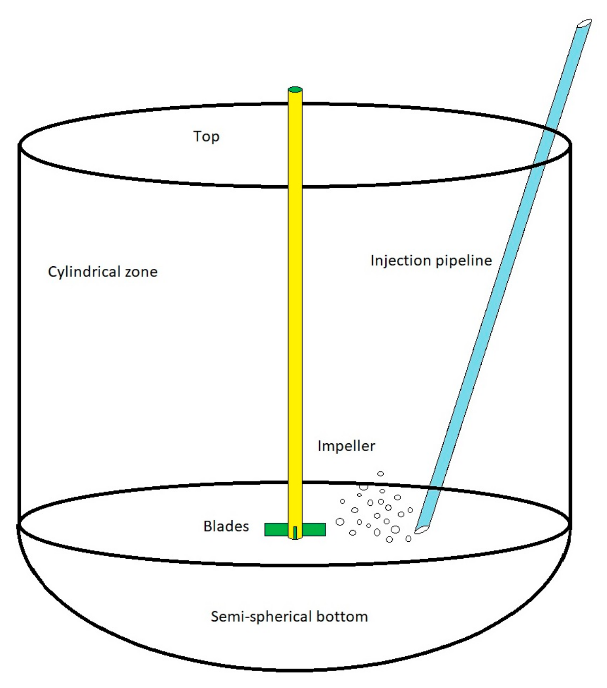
The reactor was a symmetrical tank vertically. It was formed by two sections: an upper cylindrical form and a hemispherical bottom, as shown in Figure 2a. It was built computationally, defining only the reactor wall as solid. The impeller was formed by a symmetrical vertical shaft with four flat blades in the lower part, each disposed at 90°. Both elements were discretized using nonstructured mesh formed with nodes, which could be analyzed with two-dimensional triangular cells or three-dimensional tetragonal cells. The largest cells were placed on the wall and the smallest cells were placed on the impeller blades.
A control plane was defined vertically for reference. Then, this plane was divided into two subplanes, as shown in Figure 3a,b. Here, each of the injection points was placed, and the tracer was replaced the original resident fluid, while in the second semi-plane, the monitoring points were placed. These are the points where the tracer’s concentration was measured. Both planes were placed at 180° to each other, dividing the reactor into 2 sections. There were 22 injection points distributed in the tank to evaluate the influence of the injected place on the mixing time; then, every injected point was evaluated independently. The impeller speed was the same for every simulation, and the influence of the walls on the mixing was considered at the points where the fluid impacted and changed the path. Although, there were no injection points below the impeller, because during real mixing operations the tracer was injected using a tubing inlet system submerged in the bath making this geometrical disposition complicated; nevertheless, there were some monitoring points in the reactor bottom because this zone is critical for mixing as a consequence of frequent problems with tracer diffusion in this region [1,2,3,4,5,6,20,21,22,23,24,25,26,27,30,31].
The nearest injection points for the impeller were pi18, pi19, pi17, and pi22, and the nearest injection points for the wall were pi6, pi12, pi16, and pi21. These points were placed on different positions in the injection plane to evaluate the influence of the reactor geometry and the impeller during rotation in order to identify the death zones and zones with tracer excess because both zones had evidenced poor mixing.
The walls of the reactor were joined to form a single empty volume and meshed using 1062 nonstructured, 2D triangular cells of regular size, which formed a continuous flat surface surrounding the entire lead volume. The cylindrical and hemispherical sections were measured as 0.66922 m2 and 0.28224 m2, respectively.
The impeller was a cylindrical shaft that was 0.610 m in length, with 4 blades in the lowest position that were 0.0508 m × 0.0254 m and 0.00375 thick. A finer 2D triangular mesh with 16,890 cells for discretizing the shaft and 657 cells for every blade was used. The impeller speed was 32 RPMs, and the moving rotating frame (MRF) condition was established in concordance. The computational model used for solving the domain was k-ε in the software ANSYS-Fluent (17.1).
The tank and the impeller were made with stainless-steel in order to resist the impacts of the liquid lead against the cylindrical walls, and the blades could promote the required stirring.
4. Initial Assumptions
The following assumptions and boundary conditions were established for every simulation run:
- (a)
- The influence of the shaft is not significant because it is placed in the middle of the reactor to achieve symmetrical conditions, and no vibration is assumed during rotation. Thus, the shaft is a rotatory wall in the middle of the tank without influence over the fluid dynamics;
- (b)
- The reactor walls are free of defects; as a consequence, there is no friction or drag effect; nevertheless, the path of the fluid and speed vectors can be modified due to the liquid particles impacting the walls at different angles;
- (c)
- The impeller rotatory speed is constant during the simulation. It is constant at 200 radians per minute. The impeller is submerged inside the reactor at a central position;
- (d)
- The surface of the liquid lead is flat; this means that no turbulence condition is assumed over the surface or that the tank is a closed volume;
- (e)
- The lead temperature of the liquid lead is assumed at 327 °C during the simulation, and the system is assumed as isothermal;
- (f)
- The tracer is injected in only one injection point at the start time (t = 0) for each simulation case. Thus, the tracer’s concentration at all monitoring points is equal to zero (Cm1 = Cm2, … Cm15 = 0). Moreover, the resident liquid is only lead with constant properties, and the tracer is also assumed to have the same properties as lead;
- (g)
- The velocity vectors at the beginning of the simulation are shown in Figure 4a,b, all around the tank and near the blades of the impeller, respectively. Then, a certain volume of lead is replaced with the tracer, which has the same properties as lead. Then, the fluid is assumed to be homogeneous (there are no inclusions or other fluids involved).
- (h)
- Simulations are conducted individually to analyze the hydrodynamics behavior and efficiency of the tracer’s distribution at every injection point.
Figure 4.
(a) Vectors profile inside the tank reactor considering the (a) stationary initial lead reactor; (b) final vector speed inside the tank; (c) velocity vectors at the top of the tank around the shaft of the impeller; (d) zoomed-in view of vectors near the impeller at the beginning of the stirring simulation.
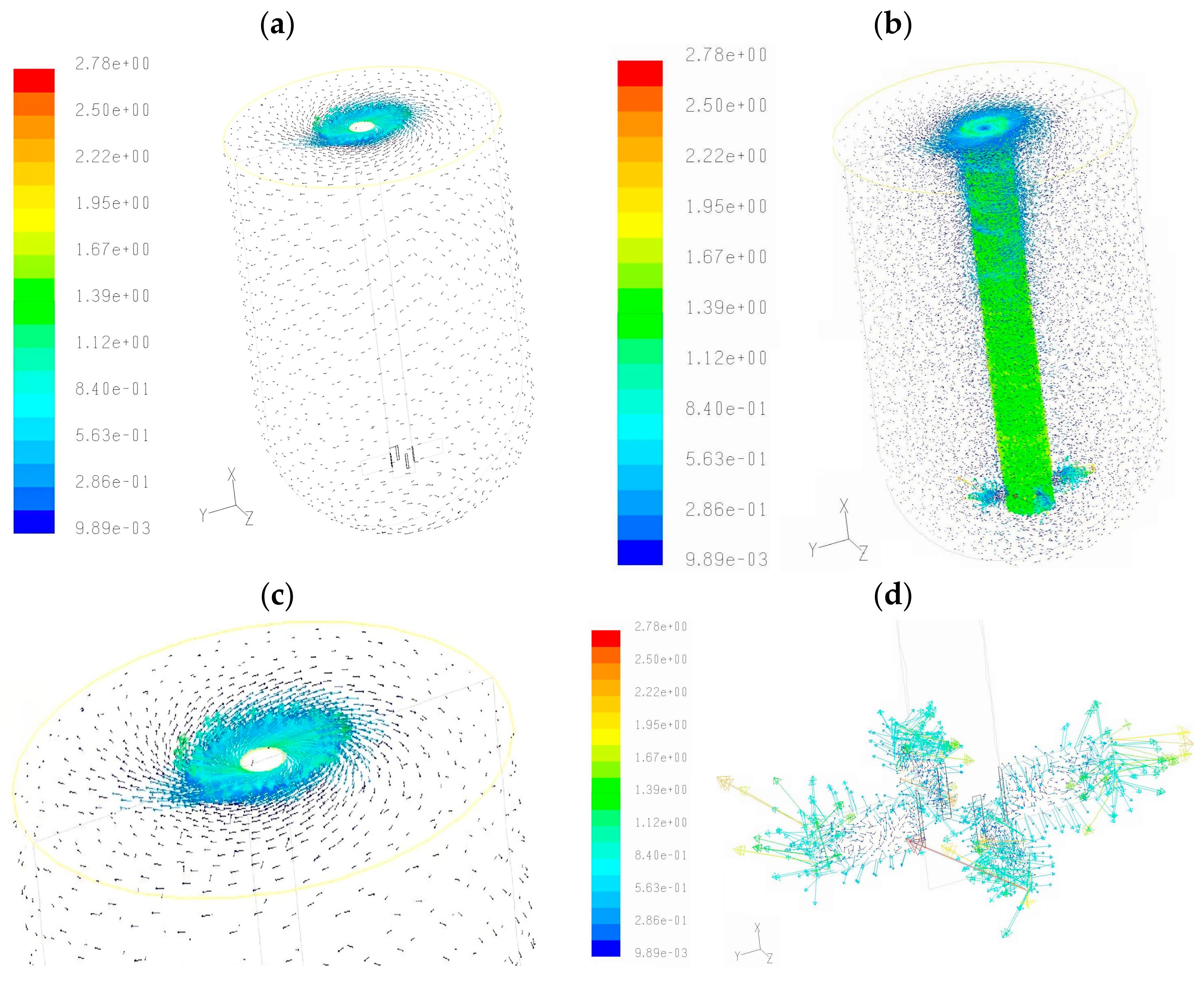
The tracer, which is initially stationary, will be distributed all around the tank reactor as the simulation is executed; then, a certain percentage of the tracer will be in every zone of the tank, and as the simulation continues the tracer will tend to be distributed homogeneously and a final value of tracer will be obtained. The injected tracer is assumed as ideal with the same physical properties as the resident lead in the tank. This condition is often used by many authors who work on physical and computer simulations [12,13,14,15,16,17,19,27,28,29,30].
Industrial agents that promote the cleaning of lead were added by plunging solids or blowing dust particles. Thus, there were no injection points below the impeller, as shown in Figure 3a; this condition is geometrically complicated and is beyond normal practices.
5. Mathematical Model
The main parameter to evaluate the mixing efficiency is the tracer’s diffusion in the entire reactor. This was evaluated by measuring the tracer’s concentration at each of the monitoring points. Equations (1) and (2) were used to evaluate the tracer’s concentration at every step time (Δt) during the simulation. Thus, when the tracer’s concentration tended to be invariable, an ideal mix was obtained. Thus, Equations (1) and (2) were the criterion for determining the invariability of the tracer’s concentration at every monitoring point; then, if the concentration at every monitoring point tended to a minimum (zero), the tracer was homogeneously distributed. Here, the superscripts (t) and (t − Δt) refer to the latest and previously calculated value of the tracer, respectively; and the subscripts (pm) and (tracer) were used to indicate that the tracer was measured at every monitoring point and as the contribution of all them, respectively. While Equation (2) indicates that the variation in the tracer’s concentration tended to a minimum, which was the criterion for considering the tracer as homogeneously distributed.
The Navier–Stokes equations are nonlinear partial differential equations that are used to describe fluid motion. Here, the nonlinearity was due to the acceleration of the fluid in motion as a consequence of the change in the velocity at each position and at every instant during the simulation. Then, Equation (3) can be rewritten using Cartesian coordinates, as shown in Equations (4)–(6). These equations were solved using the k-ε model to calculate the hydrodynamics behavior (velocity and path of fluid inside the tank).
And, the continuity equation can be written as follows:
When the flow is at a steady state, (ρ) does not change with respect to time. Then, the continuity equation is reduced to:
When the flow is incompressible, (ρ) is constant and does not change with respect to space. Then, the continuity equation is reduced to:
The velocity components (the dependent variables to be solved) are typically named u, v, and w. This system is the most commonly and formally used, though comparatively more compact than other representations; nevertheless, this is still a nonlinear system of partial differential equations for which solutions are difficult to obtain. Thus, computational representations allow for the reproduction of geometrical elements and physical conditions in detail, and numerical methods can be programed to solve complex problems concerning the flow of fluid.
The general differential equation for the mass transfer of component “A”, can be written in Cartesian coordinates as is shown in Equation (10); and, in cylindrical and spherical coordinates as Equations (11) and (12), respectively, which represent Fick’s law equations; these equations were solved for the triangular cells used for the discretization with the finite element method and a k-ε model; turbulence and diffusion are obtained. A nested routine saved the tracer’s concentration values at every monitoring point after every time step (pmt+Δt); then, the data were analyzed using Microsoft Excel. The previous equations can be used to solve regular structured or nonstructured meshes. The analyzed fluid was a mix of lead + tracer that was incorporated into the numerical solution as a multicomponent fluid problem, and Equation (13) was used to represent it [36], where Deff was the diffusion and turbulent coefficient.
6. Analysis and Efficiency of Mixing
A good mixing is considered to be obtained when the resident fluid has been homogeneously distributed throughout the entire tank. Here, the mechanical stirring system with the impeller was employed to promote mixing by adding movement to the resident fluid inside the tank.
The mixing efficiency is measured by monitoring the tracer’s concentration (Ctracer) all around the tank. During the simulation, the tracer’s concentration at each monitoring point was stored and saved (Ctpm) at every time step (t + Δt) to understand the hydrodynamics inside the tank. Different tracer concentration curves resulted at the monitoring points as a function of the influence of the impeller, the walls, and the injection point. Some of the obtained curves oscillated and then were quickly damped, and others were quasi-parabolic or overdamped, which suggests exponential decay due to the different distributions of the tracer in every zone. Consequently, in order to understand the fluid flow behavior in every zone inside the tank, an analysis considering two different injection points is shown next.
One analyzed injection point (pi1) was placed near the impeller shaft at a very high position near the tank’s top surface, and one point (pi9) was placed in the middle of the tank, as shown in Figure 3a. Figure 5, Figure 6, Figure 7, Figure 8, Figure 9, Figure 10 and Figure 11 show the tracer’s concentration in different zones inside the tank, where some curves are intentionally repeated in order to compare and then explain the hydrodynamics behavior of the liquid lead inside every zone of the tank compared with other points at vertical and lateral positions. All curves shown in these figures tended to an ideal value of the concentration Ctracer = 0.00135, which was the final tracer concentration value for considering total mixing, and the horizontal axes scales represent the required mixing time in s to obtain the final tracer concentration. Measurements of the tracer’s concentration in the tank during the simulation with the condition Ctracer > 0.00135 indicate an excess of the tracer in the region, in contrast to the condition Ctracer < 0.00135, which indicates a deficit of the tracer. Figure 5a, Figure 6a, Figure 7a, Figure 8a, Figure 9a, Figure 10a and Figure 11a correspond to the injection at point Pi1, and Figure 5b, Figure 6b, Figure 7b, Figure 8b, Figure 9b, Figure 10b and Figure 11b are for point Pi9. Figure 5c, Figure 6c, Figure 7c, Figure 8c, Figure 9c, Figure 10c and Figure 11c illustrate the analyzed zone inside the tank. Moreover, the time scales were estimated to illustrate when the final tracer concentration was reached.
The hydrodynamics behavior shown in Figure 5a,b corresponds to the top of the cylindrical section and near the upper corner of the tank. Here, a similar behavior can be identified; these curves exhibited an oscillating and irregular but quickly damped behavior; all of them had an excess of tracer concentration at the beginning, which tended to the final tracer concentration in Figure 5a. The highest tracer concentration was at the monitoring point (Pm1) because it was nearest to the injection point (Pi1); all these curves had an excess of tracer, but it was quickly distributed, and the final tracer concentration was quickly reached (no more than 50 s was required). In Figure 5b, some perturbations (suboscillating) can be observed, which may be attributed to the impact of the fluid against the flat top and cylindrical walls. Nevertheless, these small fluctuations were smoothed as the simulation continued to run. Additionally, in this figure, the curves had low tracer excess due to the injection point (Pi9) being placed in a position near the middle of the high point of the cylindrical body of the tank.
In Figure 6a, all points (pm5 to pm8) exhibited an oscillating, smoothed behavior, but the curves tended to delay achieving the final tracer concentration. The points (Pm5, Pm6 and Pm8) displayed a similar behavior because they were near the wall in the cylindrical zone, but pm7 was placed in the middle of the tank’s body. Furthermore, the oscillations were reduced in of all these curves as the simulation time increased; all of these curves showed an excess of tracer concentration, but the values were minor, as these points were far from the injection point (pi1), and the final tracer concentration was reached after 140 s.
Figure 6b shows the tracer concentration at the nearest monitoring points to injection point Pi9. Thus, Pm8 showed the highest tracer concentration value (in excess), and the second and third places were for the points Pm7 and Pm6, respectively. Here an oscillating behavior for all curves can also be observed, and the tracer excess was reduced as the monitoring point was far from the injection point. The instability due to the tracer excess was also quickly damped. This figure also shows the evolution of the tracer concentration horizontally in the middle position of the tank reactor. For the monitoring points Pm7 and Pm8, both curves had very similar behavior, evidencing they were positioned horizontally. Finally, the final tracer concentration was quickly achieved for injection point Pi9.
The next analyzed zone is in the middle but lower position on the tank. Here, the points Pm9 to Pm12 were placed near the wall of the cylindrical section of the tank near the border between the cylindrical and hemispherical zones; these points were far away from the injection point Pi1 but just below injection point Pi9. Then, as shown in Figure 7a, all curves exhibited a similar oscillating but damped behavior. The points Pm9 and Pm10 showed a moderate excess of tracer concentration, but the curves for points Pm11 and Pm12 displayed a deficit of tracer concentration. All the curves were damped, and all of the curves tended to the final tracer concentration but had a delay of nearly 300 s, and it can be noticed that the main tracer deficit appeared between the cylindrical and the hemispherical zones.
In Figure 7b, a similar oscillating damped fluid behavior can be appreciated for all of the curves. The points with the highest tracer excess were those near the injection point (Pi9). The monitoring points Pm9 and Pm10 exhibited an excess of tracer and then a strong damping can be noticed. In contrast, the monitoring points Pm11 and Pm12 were placed on the border between the cylindrical and hemispherical zones of the tank and did not have any tracer excess; thus, the damping was not as strong; moreover, these points always remained with a deficit of tracer concentration until all of them slowly tended to the final tracer concentration. Moreover, the oscillations of the tracer concentrations were stronger for the monitoring points Pm9 and Pm10, which were in the cylindrical region, than for the monitoring points Pm11 and Pm12. Finally, the curves in Figure 7b showed a similar behavior as in Figure 7a, but the curves for points Pm9 and Pm10 displayed a major excess of tracer concentration, as these were near injection point Pi9.
Figure 8a,b illustrate the hydrodynamics behavior in the hemispherical region. All of the curves in these figures were quite similar and exhibited a deficit of tracer concentration. However, an oscillating, damped behavior was displayed for the monitoring points Pm11 and Pm12 in both figures; in contrast, the curves for the points Pm13, Pm14 and Pm15 were overdamped, evidencing a very slow increment in the tracer’s concentration. Moreover, the mixing times were longer. Thus, it is possible to affirm that this is a stagnant zone. In the same way in Figure 8b, the points were placed in the deepest positions of the tank reactor. Points Pm11 and Pm12 were on the border between the cylindrical and hemispherical zones. The oscillating behavior can be noticed, but the hydrodynamics in the hemispherical zone is different, as illustrated in the curves for the points Pm13, Pm14 and Pm15. This zone is very difficult to access and the delay in distributing the tracer is long; furthermore, the tracer concentration is always deficient. Moreover, it is possible to notice that the monitoring points near the impeller were oscillating with a tracer deficit, and the points near the hemispherical wall were overdamped.
All the monitoring points tended to adopt the final tracer concentration. This is a reliable and feasible criterion for evaluating the distribution efficiency. The excess of tracer must be distributed, and the deficits must be filled all around the tank reactor for good mixing.
Excesses of tracer concentration were at the monitoring points near the corresponding injection points. But these excesses were frequently quickly distributed. In contrast, a deficit of the tracer occurred in cases where the monitoring points were placed very far from the tracer injection point or far from the impeller.
The evolution of the tracer’s concentration in the cylindrical upper wall section is shown in Figure 9a,b. All curves for the points Pm3 to Pm6 exhibited similar oscillating behavior to a family of curves; for the injection point Pi1, the monitoring points with the highest and minimum excess of tracer were Pm3 and Pm6, respectively. Although there was high tracer excess at the beginning, the final tracer concentration was quickly reached. For the injection point Pi9, the nearest monitoring point was Pm6; therefore, this point had the highest tracer excess. Here, again, an alternating oscillating behavior was also shown for all of the curves, and the damping decreased over the simulation time. Finally, all of the values tended to adopt the final tracer concentration but always with a tracer concentration in excess. Thus, the influence of the injection points can be noticed on the families of curves in Figure 9a,b; here, the curves are different for both injection points, evidencing different hydrodynamics behaviors.
The evolution of the tracer’s concentration near the cylindrical lower wall section is shown in Figure 10a,b. In Figure 10a, all curves exhibit am oscillating damped behavior; here, the monitoring points Pm8 to Pm10 display an excess of tracer concentration, but the point Pm11 show a deficit, as it is placed between the cylindrical and hemispherical zones. The excess of the tracer concentration at points Pm8 and Pm9, as shown in Figure 10a, are minor in comparison with those for the injection point Pi9 due to the injection point being far away. Finally, all curves tended to the final tracer concentration, but the delay was longer than the curves for the point Pi9. In comparison, in Figure 10b, the monitoring point Pm8 was the nearest to the injection point; thus, it had the greatest tracer concentration. Moreover, the tracer concentration was reduced from Pm8 to Pm11 as a function of the distance from the injection point. The oscillating, alternating behavior can also be observed for all of the curves. Finally, only Pm11 was, again, the only point with no tracer excess.
All of the curves with an irregular oscillating form were in the cylindrical zone, but these were damped; on the other hand, the curves with an overdamped behavior were in the hemispherical zone of the tank. The irregularity of the oscillating curves represents an excess of the tracer concentration and instability, but the tracer was quickly distributed at the monitoring point near the impeller’s influence, while the oscillating curves with a deficit of tracer were in the zones where the distribution was complicated.
The overdamped curves were always with a deficit of tracer concentration, evidencing a very slow tracer distribution; thus, these represented stagnant zones. Thus, the hemispherical region of the tank requires longer times for mixing, maybe a geometrical modification of the original tank based on hydrodynamics behavior will accelerate the tracer distribution.
The evolution of the tracer’s concentration vertically in the middle position of the tank reactor can be observed in Figure 11a,b. In Figure 11a, the monitoring points Pm2 and Pm7 exhibited an oscillating behavior. Although the tracer’s excess was quickly distributed, there was a very large difference in the tracer’s concentration for these points. On the other hand, the points Pm12 and Pm13 had deficit of tracer and showed an overdamped behavior; unfortunately, the tracer distributed slowly. In Figure 11b, the monitoring points Pm2 and Pm7 were higher than the injection point Pi9 and showed tracer excess; in contrast, the points Pm12 and Pm13 were in the hemispherical zone, evidencing a very different behavior and without any tracer excess. The curves in the middle tank were transformed from an oscillating form to an overdamped one from the upper to the lower zone of the tank.
The contributions of all of the monitoring points can be added and averaged in order to obtain one single curve for representing the hydrodynamics behavior inside the tank and evaluating the mixing efficiency as a function of the injection points. Furthermore, the resulting curves can be derived and then the final tracer concentration can be subtracted to determine if the variation of the tracer concentration tended to zero (minimum variation); this means that the tracer was homogeneously distributed. In Figure 12a,b, the curves for the analyzed injection points are shown. Here, it is possible to confirm that the injection point Pi9 was the best because the values of the tracer concentration were always minor compared to those for the point Pi1. Moreover, on the vertical axis, the derivate curve values were also minor. The average curves tended to the final tracer concentration and the derived curves tended to zero. The tendency of all curves was 0.00135, which was the volume fraction of the tracer distributed in every 3D cell where the monitoring points were placed. As a criterion for the homogeneous distribution of the tracer, it was considered that the rest of the cells used for discretization of the volume in the tank must contain the same tracer concentration. Moreover, the invariability was considered as a criterion to determine that the extra time of stirring was not necessary.
A good mixing was obtained when the tracer concentration tended to be constant (i.e., invariable). According to this criterion, the best injection point was pi18, and the worst was pi21. As is shown in Figure 13, the final tracer concentration for pi18 was quickly stabilized. This curve also shows minimized fluctuations and short periods of oscillating behavior, which were shorter than those for the other injection points. In contrast, the curve for pi21 showed a very slow tracer dispersion. The slope of this curve was soft, resulting in a homogeneous and eventually very slow tracer distribution all around the tank. This point was very far from the impeller, and the injection here was not favorable due to the diffusion problems. In this figure, the scale was modified by dividing it with the final tracer concentration; then, all curves tended to 100; a percentage that means the final tracer concentration.
The hemispherical bottom of the tank is a critical zone for mixing because the tracer distribution here involves diffusion problems and accessibility to this zone is also complicated.
Moreover, a close up at the end of the figure can be taken to show fluctuations during mixing became very short but remained; consequently, these can be neglected due to the fluctuations being nonsignificant. This concept can be appreciated in the tracer concentration profiles shown in Figure 5, Figure 6, Figure 7, Figure 8, Figure 9, Figure 10, Figure 11 and Figure 12.
7. Validation
For validation purposes, a physical model of the tank was built using transparent acrylic scaled 1:11.4 considering the lead density. The rotational speed remained constant, the fluid used was water and the tracer was NaCl. The model was sized as a function of the evaluation between the inertial and viscous forces under different velocities; then, the Reynolds number in Equation (14) was calculated at every monitoring point position and included in the computational solution, while the values of the tracer concentration were obtained from the physical modeling measured instantly using a particle indicator velocimeter (PIV).
Measurements at every monitoring point were taken using the instrument at every Δt = 0.5 s. In contrast, the time step used for the computer simulation at the smallest cells of the volume near the impeller blades was Δt = 0.0052 s resulting from the rotatory speed 1 min/32 RPM/360°. This time was considered good enough for following the evolution of the mixing process. Then, the results were saved every 10 steps to be applied on the wider mesh that discretized the tank volume.
The values of the tracer’s concentration for the physical model and computational simulation were compared for validation of the Pi18, Pi11 and Pi21. These are shown in Figure 14a–c and compared to evaluate the fidelity between both models. In this figure, the difference is evident at the beginning of the simulation but reduces as the simulation continues over time; both curves tended to the final tracer concentration. Then, it is possible to mention that the global behavior was similar. Although there were some differences between the physical and computational modeling which could have affected the resulting curves.
- (a)
- The tracer in the physical model was injected in one single amount by a blowing pipeline, as shown in Figure 15, but the impulse force was not considered in the computational model. The tracer used in the physical model was NaCl with a size between 5 × 10⁻⁴ and 7 × 10⁻⁴ m. Consequently, controlling the injection of the entire tracer in one single pulse in the physical model was difficult. The same occurs during real industrial practices;
- (b)
- The time for acquiring data in the physical model was averaged every 25 s, and the tracer was measured at every monitoring point across a plane with the same width as a tetragonal cell used for discretization in the computational model;
- (c)
- The curves of the tracer concentration (Ctracer) were the sum of all contributions of the monitoring points for the computer simulations measured independently, which were taken every 25 s for comparison in contrast to all previous figures, which were measured every 1 s.
Figure 15.
Sketch of the stirred tank built for the physical model and the injection of NaCl using a lance blowing.
Figure 15.
Sketch of the stirred tank built for the physical model and the injection of NaCl using a lance blowing.
Different mesh sizes were tested with computational modeling, including finer meshes of tetrahedral cells, hexahedral (cubic) and honey comb cells, but the final tracer concentration was so similar in all of the simulations; thus, it can be considered, again, as the moment when the tracer was homogeneously distributed.
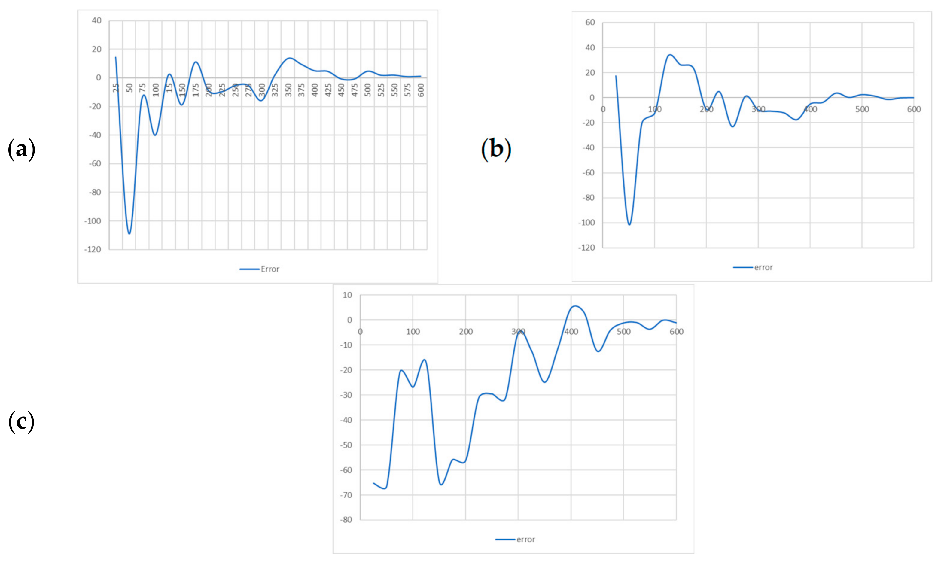
Additionally, the errors and approach were obtained using Equations (15) and (16). Here, the subscripts pi correspond to the analyzed injection point, and the superscripts (t) and (t − Δt) refer to the latest and previous tracer concentration value during the simulation. The resulting graphics are shown in Figure 16a–c and Figure 17a–c, respectively. These curves use the information on the tracer concentration in Figure 15a–c. It can be appreciated that approach improves as the tracer is homogenized inside the tank. Moreover, all of the curves tended to zero. Then, the dampening of the curves confirm that the tank was in a new stationary condition with the tracer homogeneously distributed all around.
8. Conclusions
In order to understand the hydrodynamics of fluid flow inside the tank it was observed that different tracer concentrations were measured as a function of the injection and monitoring positions. The tracer concentration measurement at monitoring points near the impeller evidenced its influence for promoting fluid displacement and tracer dispersion. Thus, after the analysis, it was possible to affirm the following facts:
The influence of the impeller was moderate at the monitoring points near the walls and at the top due to the fluid impacting against it, and the tracer was slowly distributed.
After analyzing all of the injection points, the best injection point was pi18, which was placed near the impeller and promoted a quick tracer dispersion, profiting from the force provided by the impeller.
Diffusion problems were related to the geometrical accessibility of the fluid to zones in the bottom of the tank, and here the losses of kinetic energy caused the fluid to become stagnant.
During the validation, a comparison between the tracer concentration obtained from computer simulation and the physical model showed that the error between them was reduced when the stirring process dominated the hydrodynamics; consequently, the most difficult period to simulate was the beginning of the mixing, and there was instability affecting the calculation, but the phenomenon became predictable as the tracer was homogenized.
The oscillation of the tracer concentrations was major for the monitoring points in the cylindrical region of the tank, although these oscillations were reduced the nearer to the impeller.
The smoothing of the oscillating curves indicates that the variation in the tracer concentration (Ctracer) was reduced; thus, the distribution became more homogeneous and the mixing improved. Here, the points in the middle region of the tank had a major excess of tracer than the points near the walls.
Choosing an appropriate injection point can contribute to improving the mixing and reducing the working time dramatically, eliminating unnecessary work.
Simulations over very long times when the values of the tracer concentration were not significant are not required; consequently, long working times are not required either.
Finding the best injection point proved that the mixing time can be reduced and industrial practices can be improved only by modifying this condition; nevertheless, this is a first step. For future works, the author recommends to analyze fluid hydrodynamics behavior including a complementary study with different tracer properties in order to understand if there is any other force influencing mixing like buoyancy forces; this is a necessary study because many of the slags and chemical components added to melting metals are with different properties like weight, density and viscosity. Additionally, a simulation considering an incomplete integration of the tracer in one single injection or in programmed pulses will be in better concordance with real industrial practices, in addition to modifying the geometrical configurations of the tank and impeller, including the tank’s geometrical form, number of blades, blades sizes and rotation speed of the impeller.
Funding
This research received no external funding.
Institutional Review Board Statement
Not applicable.
Data Availability Statement
Not applicable.
Acknowledgments
The authors wish to thank their institutions: Technological and Autonomous Institute of México (ITAM) and the Mexican Association of Culture and National Council of Science and Technology (CONACyT). This work is dedicated to the memory of my friend and colleague Pedro Vite-Martinez.
Conflicts of Interest
The author declares no conflict of interest.
References
- Zhang, W.; Yang, J.; Wu, X.; Hu, Y.; Yu, W.; Wang, J.; Dong, J.; Li, M.; Liang, S.; Hu, J.; et al. A critical review on secondary lead recycling technology and its prospect. Renew. Sustain. Energy Rev. 2016, 61, 108–122. [Google Scholar] [CrossRef]
- Li, Y.; Yang, S.; Taskinen, P.; He, J.; Liao, F.; Zhu, R.; Chen, Y.; Tang, C.; Wang, Y.; Jokilaakso, A. Novel recycling process for lead-acid battery paste without SO2 generation—Reaction mechanism and industrial pilot campaign. J. Clean. Prod. 2019, 217, 162–171. [Google Scholar] [CrossRef]
- Sun, Z.; Cao, H.; Zhang, X.; Lin, X.; Zheng, W.; Cao, G.; Sun, Y.; Zhang, Y. Spent lead-acid battery recycling in China—A review and sustainable analyses on mass flow of lead. Waste Manag. 2017, 64, 190–201. [Google Scholar] [CrossRef] [PubMed]
- Prengaman, R.; Mirza, A. 20—Recycling concepts for lead–acid batteries. In Lead-Acid Batteries for Future Automobiles; Elsevier: Amsterdam, The Netherlands, 2017; pp. 575–598. [Google Scholar] [CrossRef]
- Hildebrandt, T.; Osada, A.; Peng, S.; Moyer, T. 19—Standards and tests for lead–acid batteries in automotive applications. In Lead-Acid Batteries for Future Automobiles; Elsevier: Amsterdam, The Netherlands, 2017; pp. 551–573. [Google Scholar] [CrossRef]
- Moseley, P.; Rand, D.; Garche, J. 21—Lead–acid batteries for future automobiles: Status and prospect. In Lead-Acid Batteries for Future Automobiles; Elsevier: Amsterdam, The Netherlands, 2017; pp. 601–618. [Google Scholar] [CrossRef]
- Sloop, S.; Kotaich, K.; Ellis, T.; Clarke, R. RECYCLING|Lead–Acid Batteries: Electrochemical. In Encyclopedia of Electrochemical Power Sources; Elsevier: Amsterdam, The Netherlands, 2009; pp. 179–187. [Google Scholar] [CrossRef]
- Tian, X.; Gong, Y.; Wu, Y.; Agyeiwaa, A.; Zuo, T. Management of used lead acid battery in China: Secondary lead industry progress, policies and problems. Resour. Conserv. Recycl. 2014, 93, 75–84. [Google Scholar] [CrossRef]
- Blanpain, B.; Arnout, S.; Chintinne, M.; Swinbourne, D.R. Lead Recycling. In Handbook of Recycling; Elsevier: Amsterdam, The Netherlands, 2014; pp. 95–111. [Google Scholar] [CrossRef]
- Bailey, C.; Kumar, S.; Patel, M.; Piper, A.W.; Fosdick, R.A.; Hance, S. Comparison between CFD and measured data for the mixing of lead bullion. In Proceedings of the 2nd International Conference on CFD in Minerals and Process Industries CSIRO, Melbourne, Australia, 6–8 December 1999; pp. 351–356. [Google Scholar]
- Choi, B.S.; Wan, B.; Philyaw, S.; Dhanasekharan, K.; Ring, T.A. Residence Time Distributions in a Stirred Tank: Comparison of CFD Predictions with Experiment. Ind. Eng. Chem. Res. 2004, 43, 6548–6556. [Google Scholar] [CrossRef]
- Guha, D.; Ramachandran, P.; Dudukovic, M. Flow field of suspended solids in a stirred tank reactor by Lagrangian tracking. Chem. Eng. Sci. 2007, 62, 6143–6154. [Google Scholar] [CrossRef]
- Wang, F.; Mao, Z.-S.; Wang, Y.; Yang, C. Measurement of phase holdups in liquid–liquid–solid three-phase stirred tanks and CFD simulation. Chem. Eng. Sci. 2006, 61, 7535–7550. [Google Scholar] [CrossRef]
- Hartmann, H.; Derksen, J.; Akker, H.v.D. Numerical simulation of a dissolution process in a stirred tank reactor. Chem. Eng. Sci. 2006, 61, 3025–3032. [Google Scholar] [CrossRef]
- Huang, S.; Mohamad, A.; Nandakumar, K. Numerical Analysis of a Two-Phase Flow and Mixing Process in a Stirred Tank. Int. J. Chem. React. Eng. 2008, 6. [Google Scholar] [CrossRef]
- Koh, P.T.L.; Xantidis, F. CFD Modelling in the scale-up of a stirred reactor for resin beads. In Proceedings of the 2nd International Conference on CFD in Minerals and Process Industries CSIRO, Melbourne, Australia, 6–8 December 1999; pp. 369–374. [Google Scholar]
- Murthy, B.; Deshmukh, N.; Patwardhan, A.; Joshi, J. Hollow self-inducing impellers: Flow visualization and CFD simulation. Chem. Eng. Sci. 2007, 62, 3839–3848. [Google Scholar] [CrossRef]
- Zhang, Z.; Chen, G. Liquid mixing enhancement by chaotic perturbations in stirred tanks. Chaos Solitons Fractals 2008, 36, 144–149. [Google Scholar] [CrossRef]
- Colli, A.; Bisang, J. Evaluation of the hydrodynamic behaviour of turbulence promoters in parallel plate electrochemical reactors by means of the dispersion model. Electrochim. Acta 2011, 56, 7312–7318. [Google Scholar] [CrossRef]
- Zhao, H.-L.; Zhang, Z.-M.; Zhang, T.-A.; Liu, Y.; Gu, S.-Q.; Zhang, C. Experimental and CFD studies of solid–liquid slurry tank stirred with an improved Intermig impeller. Trans. Nonferrous Met. Soc. China 2014, 24, 2650–2659. [Google Scholar] [CrossRef]
- Gong, Y.; Tian, X.-M.; Wu, Y.-F.; Tan, Z.; Lv, L. Recent development of recycling lead from scrap CRTs: A technological review. Waste Manag. 2016, 57, 176–186. [Google Scholar] [CrossRef] [PubMed]
- Tamburini, A.; Cipollina, A.; Micale, G.; Brucato, A.; Ciofalo, M. Influence of drag and turbulence modelling on CFD predictions of solid liquid suspensions in stirred vessels. Chem. Eng. Res. Des. 2013, 92, 1045–1063. [Google Scholar] [CrossRef]
- Wadnerkar, D.; Tade, M.O.; Pareek, V.K.; Utikar, R.P. CFD simulation of solid–liquid stirred tanks for low to dense solid loading systems. Particuology 2016, 29, 16–33. [Google Scholar] [CrossRef]
- Karcz, J.; Cudak, M.; Szoplik, J. Stirring of a liquid in a stirred tank with an eccentrically located impeller. Chem. Eng. Sci. 2005, 60, 2369–2380. [Google Scholar] [CrossRef]
- Szalai, E.; Arratia, P.; Johnson, K.; Muzzio, F. Mixing analysis in a tank stirred with Ekato Intermig® impellers. Chem. Eng. Sci. 2004, 59, 3793–3805. [Google Scholar] [CrossRef]
- Pinho, F.; Piqueiro, F.; Proença, M.; Santos, A. Turbulent flow in stirred vessels agitated by a single, low-clearance hyperboloid impeller. Chem. Eng. Sci. 2000, 55, 3287–3303. [Google Scholar] [CrossRef]
- Vite-Martínez, P.; Durán-Valencia, C.; Cruz-Maya, J.; Ramírez-López, A.; López-Ramírez, S. Optimization of reagents injection in a stirred batch reactor by numerical simulation. Comput. Chem. Eng. 2014, 60, 307–314. [Google Scholar] [CrossRef]
- Pan, H.; Geng, Y.; Dong, H.; Ali, M.; Xiao, S. Sustainability evaluation of secondary lead production from spent lead acid batteries recycling. Resour. Conserv. Recycl. 2018, 140, 13–22. [Google Scholar] [CrossRef]
- Escudié, R.; Liné, A. Analysis of turbulence anisotropy in a mixing tank. Chem. Eng. Sci. 2006, 61, 2771–2779. [Google Scholar] [CrossRef]
- Vite-Martinez, P.; Ramirez-Lopez, A.; Romero-Serrano, A.; Chavez-Alcala, F. Improving of Mixing Efficiency in a Stirred Reactor for Lead Recycling Using Computer Simulation. Inz. Miner. 2014, 16, 25–32. [Google Scholar]
- Wadnerkar, D.; Utikar, R.P.; Tade, M.O.; Pareek, V.K. CFD simulation of solid–liquid stirred tanks. Adv. Powder Technol. 2012, 23, 445–453. [Google Scholar] [CrossRef]
- Xie, L.; Luo, Z.-H. Modeling and simulation of the influences of particle-particle interactions on dense solid–liquid suspensions in stirred vessels. Chem. Eng. Sci. 2018, 176, 439–453. [Google Scholar] [CrossRef]
- Gu, D.; Liu, Z.; Xie, Z.; Li, J.; Tao, C.; Wang, Y. Numerical simulation of solid-liquid suspension in a stirred tank with a dual punched rigid-flexible impeller. Adv. Powder Technol. 2017, 28, 2723–2734. [Google Scholar] [CrossRef]
- Jauhiainen, A.; Jonsson, L.; Sheng, D.-Y. Modelling of alloy mixing into steel. The influence of porous plug placement in the ladle bottom on the mixing of alloys into steel in a gas-stirred ladle. A comparison made by numerical simulation. Scand. J. Metall. 2001, 30, 242–253. [Google Scholar] [CrossRef]
- Chen, C.; Jonsson, L.T.I.; Tilliander, A.; Cheng, G.; Jönsson, P.G. A Mathematical Modeling Study of Tracer Mixing in a Continuous Casting Tundish. Metall. Mater. Trans. A 2014, 46, 169–190. [Google Scholar] [CrossRef]
- Zhang, Y.; Chen, C.; Lin, W.; Yu, Y.; Dianyu, E.; Wang, S. Numerical Simulation of Tracers Transport Process in Water Model of a Vacuum Refining Unit: Single Snorkel Refining Furnace. Steel Res. Int. 2020, 91, 2000022. [Google Scholar] [CrossRef]
- Ouyang, X.; Lin, W.; Luo, Y.; Zhang, Y.; Fan, J.; Chen, C.; Cheng, G. Effect of Salt Tracer Dosages on the Mixing Process in the Water Model of a Single Snorkel Refining Furnace. Metals 2022, 12, 1948. [Google Scholar] [CrossRef]
- Morales, R.D.; Calderon-Hurtado, F.A.; Chattopadhyay, K. Demystifying Underlying Fluid Mechanics of Gas Stirred Ladle Systems with Top Slag Layer Using Physical Modeling and Mathematical Modeling. ISIJ Int. 2019, 59, 1224–1233. [Google Scholar] [CrossRef]
- Rahimi, M.; Parvareh, A. CFD study on mixing by coupled jet-impeller mixers in a large crude oil storage tank. Comput. Chem. Eng. 2007, 31, 737–744. [Google Scholar] [CrossRef]
- Sossa-Echeverria, J.; Taghipour, F. Computational simulation of mixing flow of shear thinning non-Newtonian fluids with various impellers in a stirred tank. Chem. Eng. Process.—Process. Intensif. 2015, 93, 66–78. [Google Scholar] [CrossRef]
- Lassin, A.; Piantone, P.; Burnol, A.; Bodénan, F.; Chateau, L.; Lerouge, C.; Crouzet, C.; Guyonnet, D.; Bailly, L. Reactivity of waste generated during lead recycling: An integrated study. J. Hazard. Mater. 2007, 139, 430–437. [Google Scholar] [CrossRef]
- Weidenhamer, J.D.; Clement, M.L. Evidence of recycling of lead battery waste into highly leaded jewelry. Chemosphere 2007, 69, 1670–1672. [Google Scholar] [CrossRef]
- Milewska, A.; Molga, E. CFD simulation of accidents in industrial batch stirred tank reactors. Chem. Eng. Sci. 2007, 62, 4920–4925. [Google Scholar] [CrossRef]
Figure 1.
Typical concentration curves of the Residence Time Distribution Curves RTDCs showing the evolution of fluid dispersions during the mixing of liquids in chemical reactors.
Figure 1.
Typical concentration curves of the Residence Time Distribution Curves RTDCs showing the evolution of fluid dispersions during the mixing of liquids in chemical reactors.

Figure 2.
Sketch of the chemical reactor for lead recycling: (a) tank reactor; (b) impeller.

Figure 3.
Control plane inside the lead recycling reactor: (a) semi-plane used for placing the injection points: (b) semi-plane used for placing the monitoring points.
Figure 3.
Control plane inside the lead recycling reactor: (a) semi-plane used for placing the injection points: (b) semi-plane used for placing the monitoring points.

Figure 5.
Curves of the analysis of the mixing efficiency near the top (upper zone) and cylinder wall: (a) injection point Pi1; (b) injection point Pi9; (c) analyzed region inside the tank.
Figure 5.
Curves of the analysis of the mixing efficiency near the top (upper zone) and cylinder wall: (a) injection point Pi1; (b) injection point Pi9; (c) analyzed region inside the tank.

Figure 6.
Curves for the analysis of the mixing efficiency of the wall and middle points: (a) injection point Pi1; (b) injection point Pi9; (c) analyzed region inside the tank.
Figure 6.
Curves for the analysis of the mixing efficiency of the wall and middle points: (a) injection point Pi1; (b) injection point Pi9; (c) analyzed region inside the tank.

Figure 7.
Curves for the analysis of the mixing efficiency at the middle and low cylindrical zone: (a) injection point Pi1; (b) injection point Pi9; (c) analyzed region inside the tank.
Figure 7.
Curves for the analysis of the mixing efficiency at the middle and low cylindrical zone: (a) injection point Pi1; (b) injection point Pi9; (c) analyzed region inside the tank.

Figure 8.
Curves for the analysis of the mixing efficiency at the border between the cylindrical and hemispherical zones: (a) injection point Pi1; (b) injection point Pi9; (c) analyzed region inside the tank.
Figure 8.
Curves for the analysis of the mixing efficiency at the border between the cylindrical and hemispherical zones: (a) injection point Pi1; (b) injection point Pi9; (c) analyzed region inside the tank.
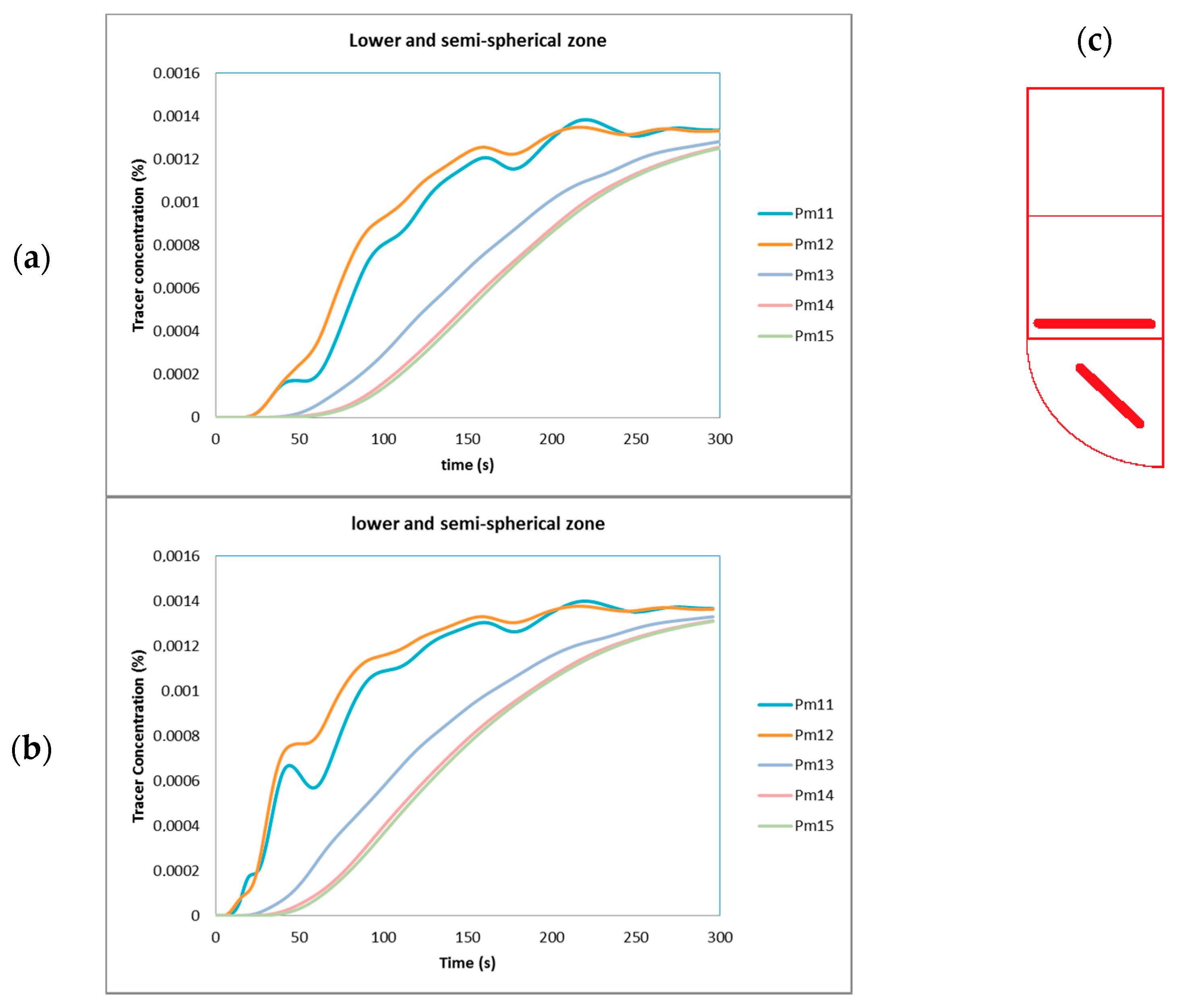
Figure 9.
Curves for the analysis of the mixing efficiency on the upper near cylindrical wall zone: (a) injection point Pi1; (b) injection point Pi9; (c) analyzed region inside the tank.
Figure 9.
Curves for the analysis of the mixing efficiency on the upper near cylindrical wall zone: (a) injection point Pi1; (b) injection point Pi9; (c) analyzed region inside the tank.

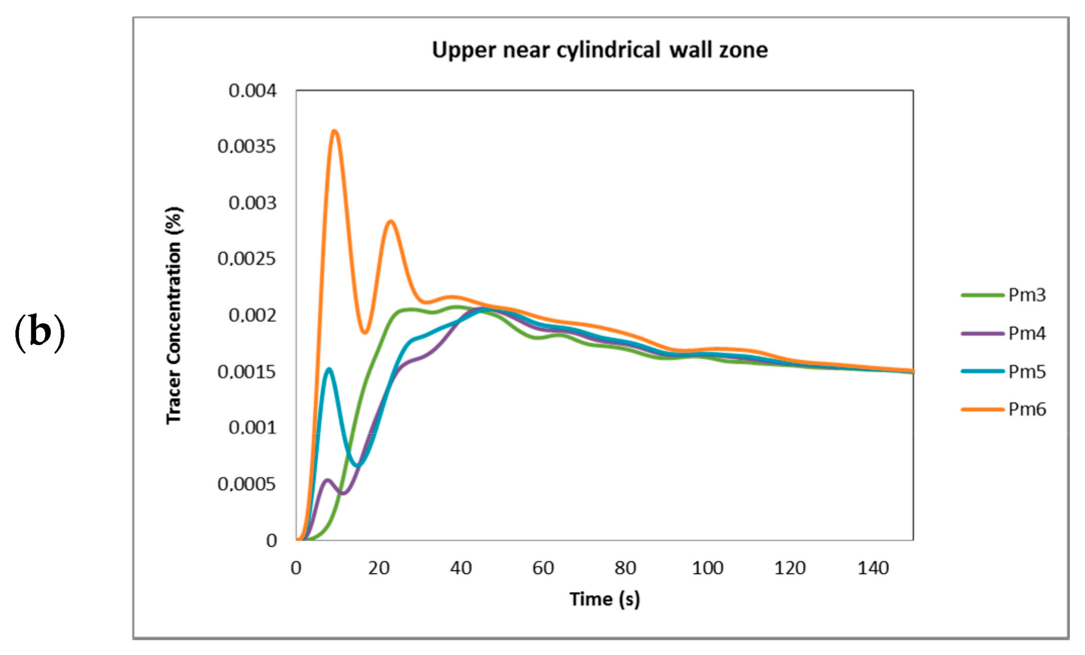
Figure 10.
Curves for the analysis of the mixing efficiency on the low and cylindrical wall zone, just below the injection point: (a) injection point Pi1; (b) injection point Pi9; (c) analyzed region inside the tank.
Figure 10.
Curves for the analysis of the mixing efficiency on the low and cylindrical wall zone, just below the injection point: (a) injection point Pi1; (b) injection point Pi9; (c) analyzed region inside the tank.

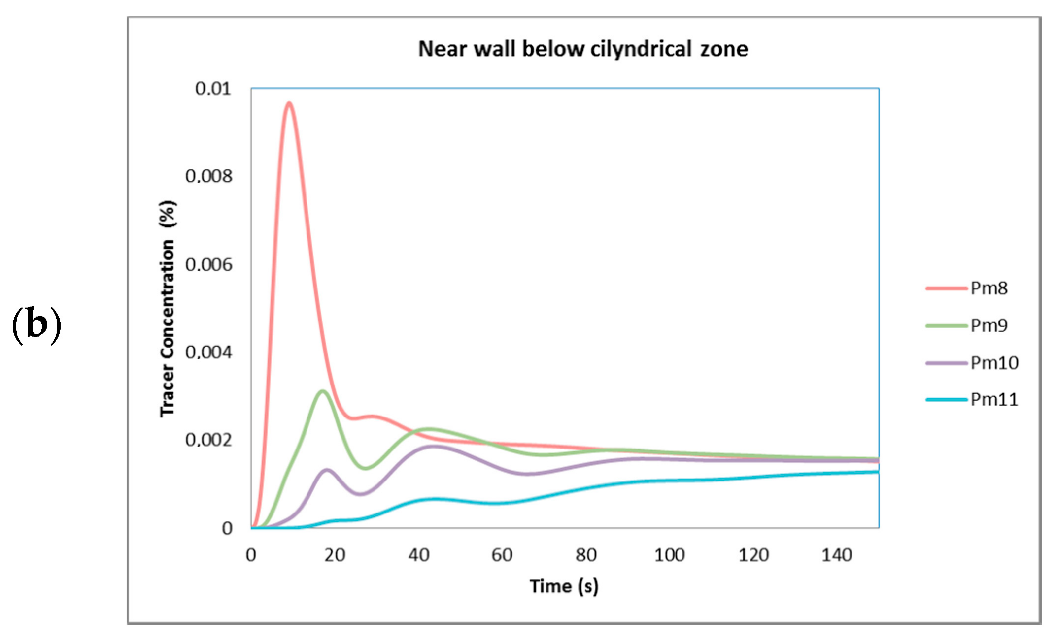
Figure 11.
Curves for the analysis of the mixing efficiency in the middle vertical zone: (a) injection point Pi1; (b) injection point Pi9; (c) analyzed region inside the tank.
Figure 11.
Curves for the analysis of the mixing efficiency in the middle vertical zone: (a) injection point Pi1; (b) injection point Pi9; (c) analyzed region inside the tank.
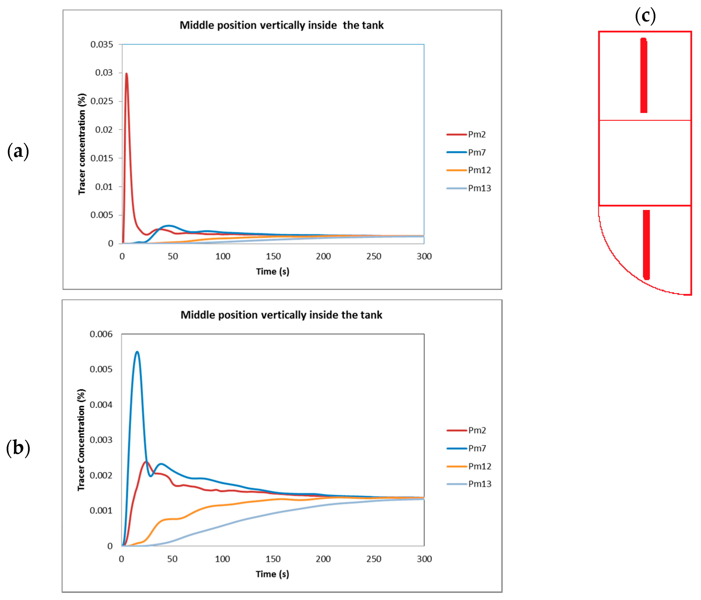
Figure 12.
Average and derivative curves for the injection points: (a) Pi1; (b) Pi9.
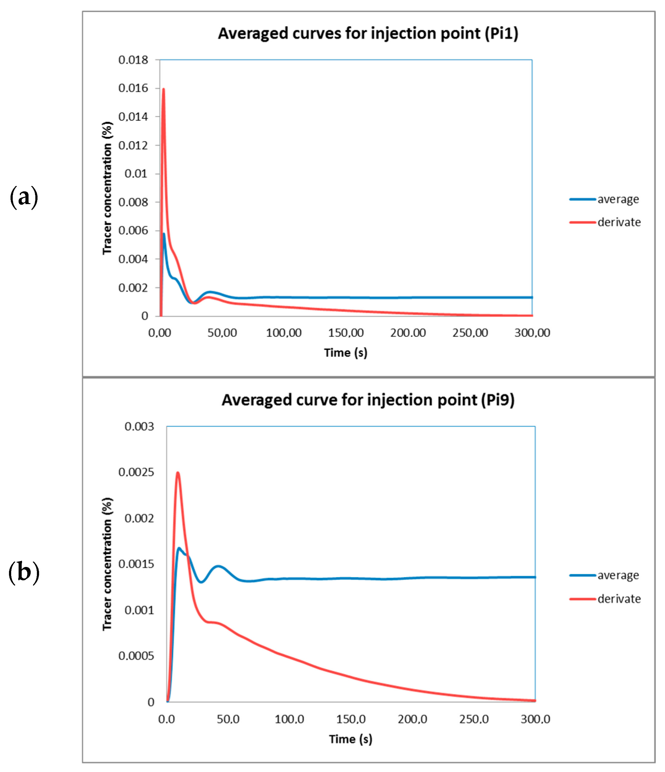
Figure 13.
Tracer concentrations for the best, intermediate and worst injection points (Pi18, Pi11 and Pi21, respectively).
Figure 13.
Tracer concentrations for the best, intermediate and worst injection points (Pi18, Pi11 and Pi21, respectively).
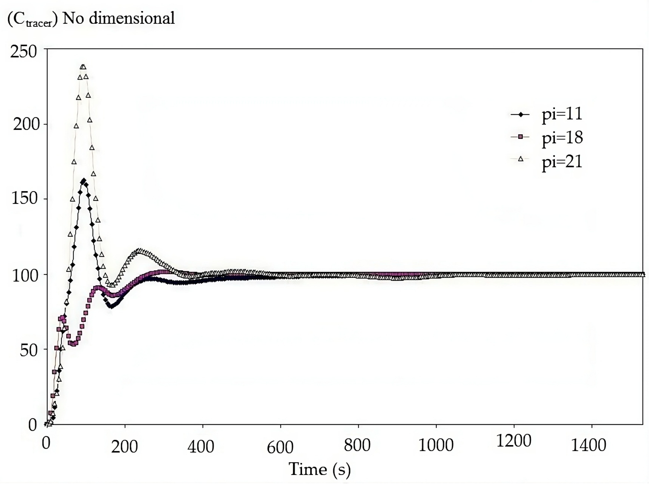
Figure 14.
Comparisons between the physical modeling and computer simulation injection points: (a) pi18; (b) pi11; (c) pi21.
Figure 14.
Comparisons between the physical modeling and computer simulation injection points: (a) pi18; (b) pi11; (c) pi21.
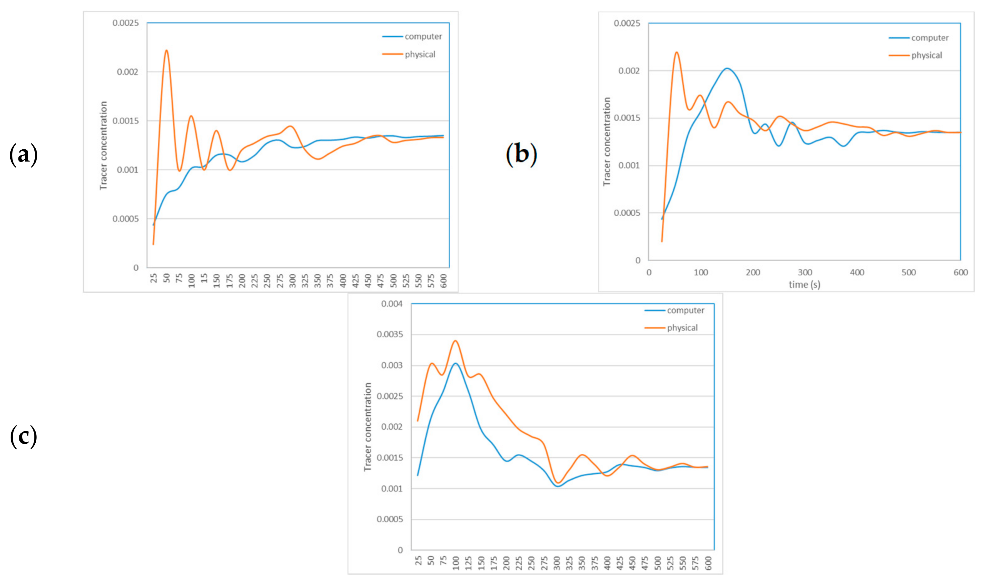
Figure 16.
Calculated errors for comparisons between the physical modeling and computer simulation as a function of the latest tracer concentration for the injection points: (a) pi18; (b) pi11; (c) pi21.
Figure 16.
Calculated errors for comparisons between the physical modeling and computer simulation as a function of the latest tracer concentration for the injection points: (a) pi18; (b) pi11; (c) pi21.

Figure 17.
Calculated errors for comparisons between the physical modeling and computer simulation for the injection points: (a) pi18; (b) pi11; (c) pi21.
Figure 17.
Calculated errors for comparisons between the physical modeling and computer simulation for the injection points: (a) pi18; (b) pi11; (c) pi21.
Disclaimer/Publisher’s Note: The statements, opinions and data contained in all publications are solely those of the individual author(s) and contributor(s) and not of MDPI and/or the editor(s). MDPI and/or the editor(s) disclaim responsibility for any injury to people or property resulting from any ideas, methods, instructions or products referred to in the content. |
© 2023 by the author. Licensee MDPI, Basel, Switzerland. This article is an open access article distributed under the terms and conditions of the Creative Commons Attribution (CC BY) license (https://creativecommons.org/licenses/by/4.0/).
Share and Cite
MDPI and ACS Style
Ramirez-Lopez, A. Analysis of the Hydrodynamics Behavior Inside a Stirred Reactor for Lead Recycling. Fluids 2023, 8, 268. https://doi.org/10.3390/fluids8100268
AMA Style
Ramirez-Lopez A. Analysis of the Hydrodynamics Behavior Inside a Stirred Reactor for Lead Recycling. Fluids. 2023; 8(10):268. https://doi.org/10.3390/fluids8100268
Chicago/Turabian StyleRamirez-Lopez, Adan. 2023. "Analysis of the Hydrodynamics Behavior Inside a Stirred Reactor for Lead Recycling" Fluids 8, no. 10: 268. https://doi.org/10.3390/fluids8100268