
Free-Decay Heave Motion of a Spherical Buoy
by
 , , and
Jacob K. Colling
, 
Saeed Jafari Kang
,
Esmaeil Dehdashti
,
Salman Husain
,
Hassan Masoud
* and
Gordon G. Parker
* Department of Mechanical Engineering-Engineering Mechanics, Michigan Technological University, Houghton, MI 49931, USA
*
Authors to whom correspondence should be addressed.
Fluids 2022, 7(6), 188; https://doi.org/10.3390/fluids7060188
Submission received: 30 March 2022
/
Revised: 20 May 2022
/
Accepted: 24 May 2022
/
Published: 27 May 2022
(This article belongs to the Special Issue Fluid Structure Interaction: Methods and Applications)
Abstract
:We examined the heave motion of a spherical buoy during a free-decay drop test. A comprehensive approach was adopted to study the oscillations of the buoy involving experimental measurements and complementary numerical simulations. The experiments were performed in a wave tank equipped with an array of high-speed motion-capture cameras and a set of high-precision wave gauges. The simulations included three sets of calculations with varying levels of sophistication. Specifically, in one set, the volume-of-fluid (VOF) method was used to solve the incompressible, two-phase, Navier–Stokes equations on an overset grid, whereas the calculations in other sets were based on Cummins and mass-spring-damper models that are both rooted in the linear potential flow theory. Excellent agreements were observed between the experimental data and the results of VOF simulations. Although less accurate, the predictions of the two reduced-order models were found to be quite credible, too. Regarding the motion of the buoy, the obtained results indicate that, after being released from a height approximately equal to its draft at static equilibrium (which is about 60% of its radius), the buoy underwent nearly harmonic damped oscillations. The conducted analysis reveals that the draft length of the buoy has a profound effect on the frequency and attenuation rate of the oscillations. For example, compared to a spherical buoy of the same size that is half submerged at equilibrium (i.e., the draft is equal to the radius), the tested buoy oscillated with a period that was roughly 20% shorter, and its amplitude of oscillations decayed almost twice faster per period. Overall, the presented study provides additional insights into the motion response of a floating sphere that can be used for optimal buoy design for energy extraction.
1. Introduction
A point absorber wave energy converter (WEC) transforms the mechanical energy of waves into either useful work or another form of energy that can be stored or transmitted. Exploiting the relative velocity between its buoy and the seafloor or a nearly stationary component in opposition to a force or torque allows for energy extraction [1]. Two example applications are supplying terrestrial power grids [2] and storing electrical energy in a marine energy grid (MEG) [3] to resupply autonomous vessels. A WEC’s power take-off (PTO) performs the conversion and can take many forms, including hydraulic or electrical machines [4,5]. While most point absorbers can passively harvest wave energy, their efficiency increases dramatically when the PTO is also used as an actuator in conjunction with closed-loop control.
For a heave-only device, a velocity feedback control strategy is an approach for increasing energy production without requiring a model of the buoy’s dynamic response [6]. In contrast, if the WEC’s wave response dynamics can be modeled, then a model-based control strategy can be used to further enhance its energy extraction. Impedance matching or complex conjugate control is one example when the point absorber operates in a linear regime. Since model terms are canceled by the control law [7], energy extraction performance increases with the greater accuracy of the WEC’s model parameters such as added mass, buoyancy force, and radiation damping. These parameters depend on the buoy’s shape, implying the opportunity for optimal shape design that harmonizes its dynamic response with a particular control strategy. Put another way, given a model-based control strategy, a family of buoy shapes and power take-off technologies likely exist that permit maximum energy extraction. Recent control algorithm development has focused on large buoy motions to exploit the buoy’s nonlinear dynamic response, further motivating the need for accurate models for control-system implementation and buoy-shape optimization [8,9,10].
To date, there have been many studies concerning the dynamics of an oscillating floating body (e.g., [11,12,13,14,15,16,17,18,19,20,21,22,23]), a large portion of which were conducted using experimental measurements, reduced-order modeling, or high-fidelity numerical simulation. A small minority of these studies, on the other hand, performed their analyses via a combination of the aforementioned methods (e.g., [24,25,26,27,28]). A recent example of such research is the work of Kramer et al. [29], where the free-decay heave oscillations of a spherical buoy were probed through several low- and high-fidelity numerical models and laboratory measurements with the goal of creating a reliable reference data set for future studies. Although very comprehensive, the reported free-decay tests were all for a sphere with the equilibrium draft length equal to its radius. The modeling and experiments presented below complement the benchmark study of Kramer et al. [29] by considering the free oscillations of a similarly-sized spherical buoy whose draft is about 60% of its radius. We find that the oscillation characteristics of the buoy are significantly influenced by its draft length at equilibrium and also demonstrate that various modeling strategies can capture this effect well.
2. Experimental Measurements
The goal of the experiments was to measure the free-decay response of a spherical buoy and the resulting water surface disturbance. The buoy was suspended above the wave tank, such that the water surface was tangential to the lowest point of the buoy at the start of each experiment. The buoy was then released and allowed to fall freely, disturbing the water surface and causing the buoy to oscillate. The position response of the buoy and the disturbance of the water surface were measured using a camera-based motion-capture system and resistance wave gauges, respectively.
The equipment used for the experiments is summarized in Table 1. The wave tank shown in Figure 1 was 10 m long, 3 m wide, and had a water depth of 1m. It was instrumented with eight resistive wave gauges and an eleven-camera Qualisys motion-capture system. The wave gauges were 0.7 m long with a measurement error of less than 0.1% of the full scale (less than 0.7 mm) and captured data at 32 Hz [30]. The mixed camera Qualisys motion-capture system used eight Oqus and three Miqus cameras capturing data at 64 Hz. The measurement accuracy of any camera-based motion capture system depends on camera locations and the calibration quality. We used the Qualisys Lab Designer to set the position of the cameras with the goal of achieving a precise coverage of the wave tank. Systems using a similar technology and our calibration strategy achieved a mean position accuracy within 0.017 mm of an externally measured reference value [31].
Two beam structures spanned the width of the tank and were used for wave gauge mounting. An additional cantilevered structure was mounted to the top of the wave tank sidewall. A wire and pulley system attached to the cantilevered structure was used to suspend and drop the buoy during the tests. The spherical buoy had a radius of 0.142 m a mass of 2.835 kg and draft of 0.090 m. Four spherical reflective markers of 19 mm radius were attached to the buoy’s top hemisphere to measure its six-degree-of-freedom rigid body motion. Eight additional markers were positioned on top of the wave gauges to measure their position in the tank. The wave gauge locations in the horizontal plane, using the buoy’s center of mass as the reference, are given in Table 2 along with their radial distances.
The buoy was suspended above the water and could be released into free-fall nearly instantaneously. The wave gauges were radially positioned around the buoy at increasing distances to capture the radiated wave created by the buoy’s release. A diagram showing a top–down view of the test setup is given in Figure 2a. An annotated image of the actual test setup is provided in Figure 2b, where each wave gauge is assigned a numerical identifier.
A total of ten experimental trials were conducted. Data collection was initiated for each trial once the water surface had no significant observable disturbances and the buoy was at rest in its initial test position. All data were time-synchronized by electronically triggering the camera and wave-gauge data-acquisition systems simultaneously. The buoy was released and allowed to fall freely into the water once the data collection had been successfully initiated. The data were collected for approximately 30 to 40 s following the buoy’s release into the water. Data collection for the trial was then ceased, and the buoy was repositioned for the next trial.
3. Numerical Simulations
The experimental measurements described in the previous section were complemented by numerical simulations. In particular, three approaches with various degrees of complexity were adopted to model the free-decay motion of the buoy. The highest-fidelity approach was based on the solution of two-phase, incompressible, Navier–Stokes equations, while the two other approaches originated from the linear potential flow theory. Specifics of the simulation methods are detailed below.
3.1. High-Fidelity Model Based on Solution of Navier–Stokes Equations
We employed the volume-of-fluid (VOF) method [32] to model the two-phase, incompressible flow of air and water. In this approach, equations that govern the spatio-temporal distribution of the average velocity and pressure fields (represented by u and p, respectively) are expressed as
where is the mixture density, t is the time variable, g is the gravitational acceleration vector, fγ is the surface tension force, and is the average stress tensor, with I and being the identity tensor and mixture viscosity, respectively. It is worth mentioning that, as shown in a number of previous studies (see [29] for a recent example), the dynamics of the buoy and the flow around it can be accurately captured without needing to include a turbulent model in the simulations. We assumed that the two-phase fluid is initially at rest (i.e., u = 0 at t = 0) and considered the boundary conditions
where is the position vector, n is the unit normal vector pointing towards the fluid, Sb represents the surface of the buoy, and St denotes the top boundary of the computational domain that confines the air column from the above. The instantaneous linear and angular velocities of the buoy (U and , respectively) were determined via
where m, , and are the mass, moment of inertia tensor, and center of mass of the buoy, respectively. Both U and were set to zero at t = 0, and the initial position of the buoy was set to its corresponding value in the experiments. Note that the contribution of surface tension to the load exerted on the buoy was ignored while still accounting for its contribution to Equation (1).
Denoting the volume fraction of water by , the average density and viscosity in the VOF model can be written as
where the water and air properties are distinguished by the subscripts w and a, respectively. The phase indicator evolves according to the advection equation
In our simulations, α was initially distributed to reflect the location of the undisturbed water level (located at z = H with H being the water height) in the experiments, i.e., α = 1 for z ≤ H and α = 0 for z > H. With α known, fγ was calculated following the continuum surface force (CSF) model [33] from
where the surface tension was assumed to be constant, and the curvature was approximated by
We used a finite-volume approach as implemented in OpenFOAM [34] to solve Equations (1) and (5). In our numerical calculations, the Laplacian and gradient operators were discretized via the second-order linear Gaussian integration, the divergence of the advective terms in Equations (1) and (5) was treated using the van Leer and linear Gaussian interpolations, respectively, the corrected scheme (with the number of corrections set to two) was used to calculate surface normal gradients, the time derivatives were approximated by the Euler scheme, and the equations of motion for the buoy were integrated using the Newmark method with the relaxation parameter set to 0.5. Moreover, the PIMPLE algorithm was employed to treat the pressure–velocity coupling, the linear solver PBiCGStab (preconditioned biconjugate gradient) with diagonal-based incomplete LU (DILU) preconditioner was used to solve for the pressure field, and the Gauss–Seidel method was utilized to calculate the velocity and phase indicator fields. The time step of the simulations was actively adjusted to keep the CFL number below 0.5 at all times.
For the purpose of maintaining the sharpness of the water–air interface during simulations, Equation (5) was modified according to the interface compression method, where an additional advective term (known as the compression term) was introduced to counterbalance excessive smearing of the interface. This extra term was integrated via the linear Gaussian interpolation scheme. Lastly, to ensure boundedness, the adapted transport equation for was solved using a semi-implicit (and second-order in time) algorithm known as multidimensional universal limiter for explicit solution (MULES).
Our computational domain was set up to match the size and geometry of the wave tank (see Figure a). For efficiency purposes, the air column above the free surface of the water was confined from above to the height of 1 m, which is large enough to permit accurate simulations. The air column was also laterally bounded through the vertical extension of the sidewalls of the tank up to the top confining boundary. We adopted an overset mesh approach [35,36,37,38,39,40,41] to discretize the simulation space and to handle the moving boundary problem resulting from the motion of the buoy. In the overset-grid method (which is also known as chimera [42,43] and overlapping-grid method [44,45,46]), the computational domain is decomposed into multiple overlapping grids. The governing equations are separately solved for each grid, and the connection between different subdomains is achieved through interpolating over the overlapping zones [47]. To implement overset gridding, we used a fixed background mesh and another one that moved with the buoy (see Figure 3b,c). Both meshes were generated via the snappyHexMesh utility of OpenFOAM in a multiblock fashion. The inverse distance weighting method was also used to carry out the interpolations over the overlapping zone.
To conclude, we note that all simulation parameters were chosen based on their corresponding experimental values. Moreover, several verification tests were performed to ensure the accuracy of the results independent of the domain size, grid resolution, and time-step duration. Specifically, regarding the grid resolution, we tested three sets of meshes with approximate total number of elements of , and . The results of the last two meshes differed only marginally, but the data presented in Section 4 were generated using the very last mesh that had the largest number of elements among the three sets.
3.2. Reduced-Order Models Based on Linear Potential Flow Theory
3.2.1. Cummins Model
A commonly accepted alternative to the accurate yet computationally demanding simulation method presented in Section 3.1 is the modeling approach of Cummins [48], where the hydrodynamic load experienced by the buoy is calculated according to the linear potential flow theory (see, e.g., [49]), while the forces due to the surface tension and airflow are ignored. The equation of motion for the heave oscillations of the buoy in this reduced-order model takes the form of
Here, Uz = dzb/dt is the velocity of the buoy in the z direction, R = 0.142 m is the buoy’s radius, and d = 0.090 m and denote the draft and the center of mass position of the buoy in the z direction at static equilibrium, respectively. The infinite frequency added mass coefficient and radiation impulse response function (IRF) in the above equation can be expressed (see, e.g., [49]), respectively, as
where and are the added mass and damping coefficients corresponding to the small-amplitude, sinusoidal, heave oscillations of the buoy with frequency about its static equilibrium position. These two coefficients are in turn calculated from
Here, , is the wet surface of the buoy at its static equilibrium, is the differential surface element nondimentionalized by R2, and is the dimensionless, complex-valued velocity potential field that satisfies the following boundary-value problem:
Note that, here, the sidewalls of the wave tank are assumed to be ideal absorbers through the application of the radiation boundary condition at large radial distances away from the buoy.
We solved Equation (11) using a second-order finite-element method as implemented in COMSOL Multiphysics [50,51]. Specifically, the outer boundary at infinity was modeled as a large cylinder of height H/R and approximate radius 300 whose center coincided with the center of the buoy. Also, triangular elements were used to discretize the 2D axisymmetric computational domain. The accuracy of this computational scheme was validated through a comparison with the theoretical calculations of Hulme [13], and through grid and domain-size independence studies.
The result of our calculations for the added mass and damping coefficients, and the impulse response function are presented in Figure 4. Having computed a∞ and k(t), we iteratively solved integro-differential Equation (8) for the position of the buoy, where at each iteration, the convolution integral was treated as a forcing function whose values were known from the velocity Uz calculated in the previous iteration. The forcing function was set to zero in the first iteration.
3.2.2. Mass-Spring-Damper Model
Less sophisticated than Cummin’s approach, the free-decay heave motion of the buoy can be approximated as:
where
Equation (12) expresses the displacement of a free harmonic oscillator with mass that is acted upon by a damper of resistance coefficient and a spring of stiffness c. Here, and are the added mass and damping coefficients corresponding to the damped natural frequency (see Equations (10) and (11)). This frequency can be calculated in an iterative fashion as follows (see also [49]):
where
and and are the coefficients associated with , which is the frequency calculated in the n-th iteration. Notably, with as few as N = 3 attempts, our calculations converged to
with a relative error of less than 0.04%.
4. Results and Discussion
Figure 5 shows the outcomes of our experimental measurements and numerical simulations. Specifically, Figure 5a presents the time evolution of the buoy’s position in the z direction over three seconds following the buoy’s release, and Figure 5b–i present the elevation of the air–water interface at eight locations surrounding the buoy (see Figure 2a,b) during the same time interval. Note that the experimental data were averaged over ten realizations. Our results indicate that the buoy underwent nearly harmonic damped oscillations with a period of roughly 0.6 s, consistent with the prediction of the mass-spring-damper model of Section 3.2.2. These oscillations generated radiation waves that perturbed the initially flat air–water interface. The instantaneous change in the elevation of the interface was captured by the distributed wave gauges, whose readings suggest that, as expected, the waves propagated outward almost radially (compare Figure 5c,d,h, which correspond to the wave gauges with similar radial distance from the buoy).
We also learn from Figure 5 that our two-phase flow simulation using the VOF method is capable of very accurately replicating the kinematics of the buoy and the wave pattern observed in the experiments. Similarly close agreements between the VOF calculations and experimental measurements for free-decay tests of a spherical buoy were also obtained by Kramer et al. [29]. However, on the basis of the reported core hours, their simulations appear to be computationally much more demanding than ours, which took only about 10 h to complete while running on 16 CPUs. The higher computational efficiency of our approach may (at least partly) be attributed to the use of overset gridding instead of mesh morphing to resolve the moving boundary problem due to the oscillations of the buoy. Additionally, Figure 5a reveals a couple of important points regarding the performance of the reduced-order models described in Section 3.2. First, we see that the result of the mass-spring-damper model closely resembles that of the Cummins model, even though the former has a considerably simpler form. Second, we observe that both models overpredict the amplitude of buoy oscillations while satisfactorily capturing the frequency of oscillations.
Our analyses indicate that the experimental data for the buoy’s position can be fitted very well by Equation (12) with ω☆ = 9.82 s−1 and δ = 1.86. Comparing these values with the ones reported in Equation (16) suggests that the reduced-order models underpredict the effective added mass and damping coefficients corresponding to the buoy’s heave motion by about 9% and 24%, respectively. This may not be surprising, since these models are based on the linear potential flow theory. However, Kramer et al. [29] reported closer agreements between the predictions of their reduced-order models and their measurements for the case where the normalized drop height, defined as , is , which is very close to its magnitude in our work that is . This discrepancy can be due to two differences between our study and the free-decay tests performed by Kramer et al. [29], namely, disparities in the draft lengths of the buoys at static equilibrium and the position of the sidewalls. The buoy is half submerged at equilibrium (i.e., d = R), and the distance between the center of the buoy to the sidewalls was roughly 28R and 43R in the experiments of Kramer et al. [29], whereas, in our case, d = 63R, and the buoy-to-wall distances were about 10R and 35R. It is worth noting that the variations in both the added mass and damping coefficients with λ are greatly affected by the mean position of the buoy’s draft line. For instance, it is known that, for a half-submerged sphere, b/ρR3ω decays to zero very rapidly as 1/λ4 when λ → ∞ (see, e.g., [13]). Yet, we found that, for our buoy, the dimensionless damping coefficient decays more slowly to zero with a rate close to 1/λ2. Overall, our findings imply that, while reduced-order models are generally accurate, the extent to which their predictions deviate from the measurements or the results of high-fidelity models depends on the specific configuration of the problem under consideration.
5. Conclusions
The free-decay responses of a spherical buoy and its water domain were explored in both simulation and experiments. The buoy was designed such that its draft was not equal to its radius. Three levels of model fidelity were used: VOF, Cummins, and a mass-spring-damper approach. The VOF model provided the best prediction of the buoy response while also predicting the water response. It was found that using an overlapping mesh approach, in contrast to the mesh morphing strategy of [29], was noticeably more computationally efficient. The Cummins and the mass-spring-damper models also produced reasonable estimates of the buoy’s oscillation frequency and damping. The mass-spring-damper underpredicted both the added mass and damping coefficients. It should be noted that the mass-spring-damper model parameters were developed using an analytical approach without relying on experimental data fitting.
The buoy’s draft at equilibrium, about d = 63R, resulted in a roughly two-fold increase in the decay rate per period as compared to the d = R case in [29]. All three models predicted this, but with much greater accuracy by the VOF approach. Since the draft influences a buoy’s dynamic response, its effect should be considered either in optimal shape design or adaptively by the point absorber control system. Furthermore, the VOF modeling approach can be used as a surrogate for wave tank testing during buoy shape and control design processes [52].
Author Contributions
Conceptualization, project administration, methodology, data curation, and formal analysis, H.M. and G.G.P.; investigation, J.K.C., S.J.K., E.D., S.H., H.M. and G.G.P.; experiment, J.K.C.; software, S.J.K. and E.D.; writing—original draft preparation, J.K.C., S.H., H.M. and G.G.P.; writing—review and editing, H.M. and G.G.P. All authors have read and agreed to the submitted version of the manuscript.
Funding
This research received no external funding.
Data Availability Statement
Not applicable.
Acknowledgments
Partial support from the Center for Agile and Interconnected Microgrids (AIM) at Michigan Technological University (MTU) is acknowledged. This research was carried out in part using the computational resources provided by the Superior high-performance computing facility at MTU.
Conflicts of Interest
The authors declare no conflict of interest.
References
- Korde, U.A.; Ringwood, J. Hydrodynamic Control of Wave Energy Devices; Cambridge University Press: Cambridge, UK, 2016. [Google Scholar]
- Forehand, D.I.M.; Kiprakis, A.E.; Nambiar, A.J.; Wallace, A.R. A fully coupled wave-to-wire model of an array of wave energy converters. IEEE Trans. Sustain. Energy 2015, 7, 118–128. [Google Scholar] [CrossRef] [Green Version]
- Husain, S.; Parker, G.G. Effects of Hydrodynamic Coupling on Energy Extraction Performance of Wave Energy Converter Arrays. In Proceedings of the OCEANS MTS/IEEE, Charleston, SC, USA, 22–25 October 2018; pp. 1–8. [Google Scholar]
- Drew, B.; Plummer, A.R.; Sahinkaya, M.N. A review of wave energy converter technology. Proc. Inst. Mech. Eng. A J. Power Energy 2009, 223, 887–902. [Google Scholar] [CrossRef] [Green Version]
- Hansen, R.H.; Kramer, M.M.; Vidal, E. Discrete displacement hydraulic power take-off system for the wavestar wave energy converter. Energies 2013, 6, 4001–4044. [Google Scholar] [CrossRef]
- Wang, L.; Isberg, J. Nonlinear passive control of a wave energy converter subject to constraints in irregular waves. Energies 2015, 8, 6528–6542. [Google Scholar] [CrossRef] [Green Version]
- Mei, C.C. Power extraction from water waves. J. Sh. Res. 1976, 20, 63–66. [Google Scholar] [CrossRef]
- Demonte Gonzalez, T.; Parker, G.G.; Anderlini, E.; Weaver, W.W. Sliding mode control of a nonlinear wave energy converter model. J. Mar. Sci. Eng. 2021, 9, 951. [Google Scholar] [CrossRef]
- Richter, M.; Magana, M.E.; Sawodny, O.; Brekken, T.K. Nonlinear model predictive control of a point absorber wave energy converter. IEEE Trans. Sustain. Energy 2012, 4, 118–126. [Google Scholar] [CrossRef]
- Wilson, D.G.; Robinett, R.D.; Bacelli, G.; Abdelkhalik, O.; Coe, R.G. Extending Complex Conjugate Control to Nonlinear Wave Energy Converters. J. Mar. Sci. Eng. 2020, 8, 84. [Google Scholar] [CrossRef] [Green Version]
- Havelock, T.H. Waves due to a floating sphere making periodic heaving oscillations. Proc. Royal Soc. Lond. A 1955, 231, 1–7. [Google Scholar]
- Mei, C.C. Numerical methods in water-wave diffraction and radiation. Annu. Rev. Fluid Mech. 1978, 10, 393–416. [Google Scholar] [CrossRef]
- Hulme, A. The wave forces acting on a floating hemisphere undergoing forced periodic oscillations. J. Fluid Mech. 1982, 121, 443–463. [Google Scholar] [CrossRef]
- Evans, D.V.; McIver, P. Added mass and damping of a sphere section in heave. Appl. Ocean Res. 1984, 6, 45–53. [Google Scholar] [CrossRef]
- Wolgamot, H.A.; Fitzgerald, C.J. Nonlinear hydrodynamic and real fluid effects on wave energy converters. Proc. Inst. Mech. Eng. A J. Power Energy 2015, 229, 772–794. [Google Scholar] [CrossRef]
- Mercadé Ruiz, P.; Ferri, F.; Kofoed, J.P. Experimental validation of a wave energy converter array hydrodynamics tool. Sustainability 2017, 9, 115. [Google Scholar] [CrossRef]
- Penalba, M.; Giorgi, G.; Ringwood, J.V. Mathematical modelling of wave energy converters: A review of nonlinear approaches. Renew. Sustain. Energy Rev. 2017, 78, 1188–1207. [Google Scholar] [CrossRef] [Green Version]
- Windt, C.; Davidson, J.; Ringwood, J.V. High-fidelity numerical modelling of ocean wave energy systems: A review of computational fluid dynamics-based numerical wave tanks. Renew. Sustain. Energy Rev. 2018, 93, 610–630. [Google Scholar] [CrossRef] [Green Version]
- Sheng, W. Wave energy conversion and hydrodynamics modelling technologies: A review. Renew. Sustain. Energy Rev. 2019, 109, 482–498. [Google Scholar] [CrossRef]
- Konispoliatis, D.N.; Mavrakos, S.A.; Katsaounis, G.M. Theoretical evaluation of the hydrodynamic characteristics of arrays of vertical axisymmetric floaters of arbitrary shape in front of a vertical breakwater. J. Mar. Sci. Eng. 2020, 8, 62. [Google Scholar] [CrossRef] [Green Version]
- Ransley, E.; Yan, S.; Brown, S.; Hann, M.; Graham, D.; Windt, C.; Schmitt, P.; Davidson, J.; Ringwood, J.; Musiedlak, P.H.; et al. A blind comparative study of focused wave interactions with floating structures (CCP-WSI Blind Test Series 3). Int. J. Offshore Polar Eng. 2020, 30, 1–10. [Google Scholar] [CrossRef] [Green Version]
- Windt, C.; Davidson, J.; Ransley, E.J.; Greaves, D.; Jakobsen, M.; Kramer, M.; Ringwood, J.V. Validation of a CFD-based numerical wave tank model for the power production assessment of the wavestar ocean wave energy converter. Renew. Energy 2020, 146, 2499–2516. [Google Scholar] [CrossRef]
- Ransley, E.J.; Brown, S.A.; Hann, M.; Greaves, D.M.; Windt, C.; Ringwood, J.; Davidson, J.; Schmitt, P.; Yan, S.; Wang, J.X.; et al. Focused wave interactions with floating structures: A blind comparative study. Proc. Inst. Civ.-Eng.-Eng. Comput. Mech. 2021, 174, 46–61. [Google Scholar] [CrossRef]
- Zurkinden, A.S.; Ferri, F.; Beatty, S.; Kofoed, J.P.; Kramer, M. Non-linear numerical modeling and experimental testing of a point absorber wave energy converter. Ocean Eng. 2014, 78, 11–21. [Google Scholar] [CrossRef]
- Tampier, G.; Grueter, L. Hydrodynamic analysis of a heaving wave energy converter. Int. J. Mar. Energy 2017, 19, 304–318. [Google Scholar] [CrossRef]
- Têtu, A.; Ferri, F.; Kramer, M.B.; Todalshaug, J.H. Physical and mathematical modeling of a wave energy converter equipped with a negative spring mechanism for phase control. Energies 2018, 11, 2362. [Google Scholar] [CrossRef] [Green Version]
- Xu, Q.; Li, Y.; Yu, Y.H.; Ding, B.; Jiang, Z.; Lin, Z.; Cazzolato, B. Experimental and numerical investigations of a two-body floating-point absorber wave energy converter in regular waves. J. Fluids Struct. 2019, 91, 102613. [Google Scholar] [CrossRef]
- Beatty, S.J.; Bocking, B.; Bubbar, K.; Buckham, B.J.; Wild, P. Experimental and numerical comparisons of self-reacting point absorber wave energy converters in irregular waves. Ocean Eng. 2019, 173, 716–731. [Google Scholar] [CrossRef]
- Kramer, M.B.; Andersen, J.; Thomas, S.; Bendixen, F.B.; Bingham, H.; Read, R.; Holk, N.; Ransley, E.; Brown, S.; Yu, Y.H.; et al. Highly accurate experimental heave decay tests with a floating sphere: A public benchmark dataset for model validation of fluid–structure interaction. Energies 2021, 14, 269. [Google Scholar] [CrossRef]
- Edinburgh Designs Ltd. The Edinburgh Designs WG8USB Wave Gauge Controller. Available online: http://www4.edesign.co.uk/product/wavegauges (accessed on 11 September 2021).
- Vicon. Vicon Study of Dynamic Object Tracking Accuracy. Available online: https://www.vicon.com/cms/wp-content/uploads/2021/01/PS4933_Standard-Individual-Case-Study_16_Vicon-Dynamic-Object-Tracking-Accuracy.pdf (accessed on 11 September 2021).
- Hirt, C.W.; Nichols, B.D. Volume of fluid (VOF) method for the dynamics of free boundaries. J. Comput. Phys. 1981, 39, 201–225. [Google Scholar] [CrossRef]
- Brackbill, J.U.; Kothe, D.B.; Zemach, C. A continuum method for modeling surface tension. J. Comput. Phys. 1992, 100, 335–354. [Google Scholar] [CrossRef]
- Moukalled, F.; Mangani, L.; Darwish, M. The Finite Volume Method in Computational Fluid Dynamics: An Advanced Introduction with OpenFOAM® and Matlab®; Springer: Berlin/Heidelberg, Germany, 2015; Volume 113. [Google Scholar]
- Griffith, B.E.; Patankar, N.A. Immersed Methods for Fluid–Structure Interaction. Annu. Rev. Fluid Mech. 2020, 52, 421–448. [Google Scholar] [CrossRef] [Green Version]
- Freitas, C.J.; Runnels, S.R. Simulation of fluid–structure interaction using patched-overset grids. J. Fluid. Struct. 1999, 13, 191–207. [Google Scholar] [CrossRef]
- Chan, W.M. Overset grid technology development at NASA Ames Research Center. Comput. Fluids 2009, 38, 496–503. [Google Scholar] [CrossRef]
- Tang, H.S.; Jones, S.C.; Sotiropoulos, F. An overset-grid method for 3D unsteady incompressible flows. J. Comput. Phys. 2003, 191, 567–600. [Google Scholar] [CrossRef]
- Deng, H.B.; Xu, Y.Q.; Chen, D.D.; Dai, H.; Wu, J.; Tian, F.B. On numerical modeling of animal swimming and flight. Comput. Mech. 2013, 52, 1221–1242. [Google Scholar] [CrossRef]
- Shen, Z.; Wan, D.; Carrica, P.M. Dynamic overset grids in OpenFOAM with application to KCS self-propulsion and maneuvering. Ocean Eng. 2015, 108, 287–306. [Google Scholar] [CrossRef]
- Meakin, R. Moving body overset grid methods for complete aircraft tiltrotor simulations. In Proceedings of the 11th Computational Fluid Dynamics Conference, Orlando, FL, USA, 6–9 July 1993; p. 3350. [Google Scholar]
- Steger, J.L.; Dougherty, F.C.; Benek, J.A. A chimera grid scheme. Multiple overset body-conforming mesh system for finite difference adaptation to complex aircraft configurations. Adv. Grid Gener. 1983, 59–69. [Google Scholar]
- Hubbard, B.; Chen, H.C. A Chimera scheme for incompressible viscous flows with application to submarine hydrodynamics. In Proceedings of the Fluid Dynamics Conference, Colorado Springs, CO, USA, 20–23 June 1994; p. 2210. [Google Scholar]
- Chesshire, G.; Henshaw, W.D. Composite overlapping meshes for the solution of partial differential equations. J. Comput. Phys. 1990, 90, 1–64. [Google Scholar] [CrossRef]
- Henshaw, W.D.; Schwendeman, D.W. Parallel computation of three-dimensional flows using overlapping grids with adaptive mesh refinement. J. Comput. Phys. 2008, 227, 7469–7502. [Google Scholar] [CrossRef] [Green Version]
- Henshaw, W.D. Adaptive Mesh and Overlapping Grid Methods. In Encyclopedia of Aerospace Engineering; John Wiley & Sons, Ltd.: Hoboken, NJ, USA, 2010. [Google Scholar]
- Sherer, S.E.; Scott, J.N. High-order compact finite-difference methods on general overset grids. J. Comput. Phys. 2005, 210, 459–496. [Google Scholar] [CrossRef]
- Cummins, W.E. The impulse response function and ship motions. Schiffstechnik 1962, 47, 101–109. [Google Scholar]
- Falnes, J. Ocean Waves and Oscillating Systems: Linear Interactions Including Wave-Energy Extraction; Cambridge University Press: Cambridge, UK, 2002. [Google Scholar]
- Zimmerman, W.B.J. Multiphysics Modeling with Finite Element Methods; World Scientific Publishing Company: Singapore, 2006. [Google Scholar]
- Pepper, D.W.; Heinrich, J.C. The Finite Element Method: Basic Concepts and Applications with MATLAB, MAPLE, and COMSOL; CRC Press: New York, NY, USA, 2017. [Google Scholar]
- Zou, S.; Abdelkhalik, O. A numerical simulation of a variable-shape buoy wave energy converter. J. Mar. Sci. Eng. 2021, 9, 625. [Google Scholar] [CrossRef]
Figure 1.
The Edinburgh Designs wave tank at Michigan Tech’s MWave Laboratory.

Figure 2.
(a) Diagram of experimental setup (top–down view). (b) Annotated image of the experimental setup with assigned wave gauge numbers.
Figure 2.
(a) Diagram of experimental setup (top–down view). (b) Annotated image of the experimental setup with assigned wave gauge numbers.

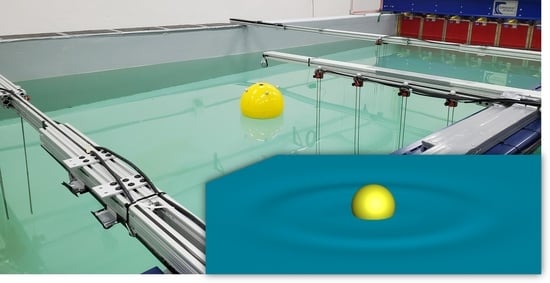
Figure 3.
(a) Representative snapshot from numerical simulations illustrating the wave created as a result of buoy oscillations. (b) Discretization of the entire computational domain and (c) a close-up view of the overset mesh around the buoy.
Figure 3.
(a) Representative snapshot from numerical simulations illustrating the wave created as a result of buoy oscillations. (b) Discretization of the entire computational domain and (c) a close-up view of the overset mesh around the buoy.


Figure 4.
Plots of the dimensionless (a) added mass and (b) damping coefficients (see Equation (10) for the definitions) versus the dimensionless parameter . (c) Plot of impulse response function (IRF) as a function of time.
Figure 4.
Plots of the dimensionless (a) added mass and (b) damping coefficients (see Equation (10) for the definitions) versus the dimensionless parameter . (c) Plot of impulse response function (IRF) as a function of time.

Figure 5.
(a) Comparison between experimental measurement and three types of numerical calculations for the time evolution of the vertical position of the buoy. (b) Comparison between experimental measurements and VOF calculations for the time history of the vertical position of the air–water interface at eight locations near the buoy. Experimental data represent averages over ten realizations, where the coefficient of variation (the ratio of the standard deviation to the mean) for the vast majority of the collected data was below a few percentage points. Subfigures (b–i) correspond to wave gauges 1–8 (see Figure 2a,b). The mean absolute differences between the plots presented here are reported in Table 3.


Table 1.
Experimental apparatus summary.
| Item | Purpose |
|---|---|
| Edinburgh Designs wave tank () | Pool for experiments |
| Eight resistive wave gauges | Water height measurement |
| Eleven-camera Qualisys motion tracking system | Buoy motion measurement |
| Spherical buoy | Test article |
| Twelve 19 mm reflective markers | Motion tracking |
Table 2.
Wave gauge positions relative to the buoy center.
| Wave Gauge Index | X Position (m) | Y Position (m) | |
|---|---|---|---|
| 1 | 1.393 | 0.004 | 1.393 |
| 2 | 1.292 | 0.004 | 1.292 |
| 3 | 0.027 | 1.159 | 1.159 |
| 4 | 0.025 | 0.950 | 0.950 |
| 5 | 0.023 | 0.705 | 0.705 |
| 6 | 0.017 | 0.458 | 0.458 |
| 7 | −1.293 | 0.019 | 1.293 |
| 8 | −1.394 | 0.021 | 1.394 |
Table 3.
Mean absolute differences between the curves plotted in Figure 5.
Table 3.
Mean absolute differences between the curves plotted in Figure 5.
| aexp-vof | aexp-Cumm | aexp-msd | b | c | d | e | f | g | h | i |
|---|---|---|---|---|---|---|---|---|---|---|
| 0.0028 | 0.0041 | 0.0045 | 0.0008 | 0.0010 | 0.0012 | 0.0015 | 0.0018 | 0.0023 | 0.0007 | 0.0006 |
Publisher’s Note: MDPI stays neutral with regard to jurisdictional claims in published maps and institutional affiliations. |
© 2022 by the authors. Licensee MDPI, Basel, Switzerland. This article is an open access article distributed under the terms and conditions of the Creative Commons Attribution (CC BY) license (https://creativecommons.org/licenses/by/4.0/).
Share and Cite
MDPI and ACS Style
Colling, J.K.; Jafari Kang, S.; Dehdashti, E.; Husain, S.; Masoud, H.; Parker, G.G. Free-Decay Heave Motion of a Spherical Buoy. Fluids 2022, 7, 188. https://doi.org/10.3390/fluids7060188
AMA Style
Colling JK, Jafari Kang S, Dehdashti E, Husain S, Masoud H, Parker GG. Free-Decay Heave Motion of a Spherical Buoy. Fluids. 2022; 7(6):188. https://doi.org/10.3390/fluids7060188
Chicago/Turabian StyleColling, Jacob K., Saeed Jafari Kang, Esmaeil Dehdashti, Salman Husain, Hassan Masoud, and Gordon G. Parker. 2022. "Free-Decay Heave Motion of a Spherical Buoy" Fluids 7, no. 6: 188. https://doi.org/10.3390/fluids7060188