
Air Entrainment in Drop Shafts: A Novel Approach Based on Machine Learning Algorithms and Hybrid Models


Department of Civil and Mechanical Engineering, University of Cassino and Southern Lazio, 03043 Cassino, Italy
*
Author to whom correspondence should be addressed.
Fluids 2022, 7(1), 20; https://doi.org/10.3390/fluids7010020
Submission received: 4 December 2021
/
Revised: 27 December 2021
/
Accepted: 28 December 2021
/
Published: 1 January 2022
(This article belongs to the Special Issue Multiphase Flow in Pipes with and without Porous Media)
Abstract
:Air entrainment phenomena have a strong influence on the hydraulic operation of a plunging drop shaft. An insufficient air intake from the outside can lead to poor operating conditions, with the onset of negative pressures inside the drop shaft, and the choking or backwater effects of the downstream and upstream flows, respectively. Air entrainment phenomena are very complex; moreover, it is impossible to define simple functional relationships between the airflow and the hydrodynamic and geometric variables on which it depends. However, this problem can be correctly addressed using prediction models based on machine learning (ML) algorithms, which can provide reliable tools to tackle highly nonlinear problems concerning experimental hydrodynamics. Furthermore, hybrid models can be developed by combining different machine learning algorithms. Hybridization may lead to an improvement in prediction accuracy. Two different models were built to predict the overall entrained airflow using data obtained during an extensive experimental campaign. The models were based on different combinations of predictors. For each model, four different hybrid variants were developed, starting from the three individual algorithms: KStar, random forest, and support vector regression. The best predictions were obtained with the model based on the largest number of predictors. Moreover, across all variants, the one based on all three algorithms proved to be the most accurate.
1. Introduction
Drop shafts are widely present in urban drainage systems, characterized by high slopes of the basins, where there is the need to reduce the flow velocities in pipes. In recent years, plunging-flow drop shafts have been the subject of some relevant literature studies [1,2,3,4,5,6,7]. Christodoulou [1] found that the local head-loss coefficient in a circular drop manhole in supercritical flows depends on a dimensionless drop parameter, expressed in terms of the drop height and the inflow velocity. Rajaratnam et al. [2] carried out experimental observations of flow features crossing a circular drop shaft and conducted measurements of energy dissipation and airflow. Chanson [3] focused on flow regimes, energy dissipation, and recirculation times in rectangular drop shafts. This study showed that rectangular drop shafts with 90° outflow are the most efficient energy dissipators. Carvalho and Leandro [4] investigated the effects of a free jet in a square drop manhole with a downstream control gate. They found that energy dissipation and turbulence, respectively, decrease and increase by raising the water discharge from the inlet and by opening the gate. Granata et al. [5] tested two specific jet-breaker devices to improve flow conditions in circular drop manholes. Jet breakers proved to be particularly effective under the worst operating conditions of the manholes. Granata [6] investigated the basic flow patterns in a drop-shaft cascade, showing that, as regards energy dissipation and air entrainment, a cascade is a more efficient solution for the single drop manhole with the same total drop height. Ma et al. [7] compared a single drop manhole with a previously reported stacked drop manhole in terms of energy dissipation, finding that the two different structures have a similar performance in energy dissipation.
The hydraulic operation of a plunging drop shaft is strongly influenced by the air entrainment phenomena that can be observed inside it. Insufficient air inlet from the outside may lead to poor operating conditions, characterized by the choking of the downstream flow, the onset of negative pressure inside the drop shaft, and backwater effects in the upstream flow. Air entrainment, in turn, changes with the operating condition.
The operating conditions of a circular drop shaft, also called flow regimes, were characterized by Granata et al. [8], who also introduced the impact number I to predict the onset of the different regimes as follows:
where s is the drop height, g is the gravitational acceleration, Vo is the average approach flow velocity, and DM is the drop shaft diameter.
In a later study, Granata et al. [9] characterized the air entrainment mechanisms typically observed in a circular drop shaft, also indicating which of them act under each flow regime. In particular, five main air entrainment mechanisms were described in the aforementioned study: The air entrainment action by the free-falling jet, the jet plunging into the bottom pool, the entrainment mechanism due to the water veil flowing along the shaft wall, the entrainment induced by the droplets released after the jet break-up, and the entrainment mechanism due to pool surface fluctuations. More details on flow regimes and air entrainment mechanisms can be found in [8] and [9]. In the latter study [9], typical results of manhole air demand measurements were shown. Moreover, it was proved that maximum air demand from outside is significantly affected by incoming flow kinetic energy and by manhole geometry. In addition, an empirical equation that allows estimating peak air demand was proposed.
Other valuable results on air entrainment in drop shafts can be found in the work of Ma et al. [10], who focused on tall plunging drop shafts. Air entrainment phenomena have been more extensively studied in vortex drop shafts, but these studies are not considered here because they are beyond the limits of this study.
The problem that has remained largely unsolved up to now is that of obtaining sufficiently accurate forecasting models of the overall air demand of a circular plunging drop shaft in any operating condition. Due to the high physical complexity of air entrainment phenomena and the impossibility of defining simple functional relationships between the airflow and the hydrodynamic and geometric variables on which it depends, the problem can be effectively addressed through machine learning (ML) algorithms. In the field of water engineering, these algorithms find their main area of application in the prediction of hydrological quantities; however, in recent years, they have also been increasingly used to tackle problems concerning experimental hydrodynamics. There have been several applications of ML in the context of studies on weirs [11,12,13,14] and scour in various fields [15,16,17]. However, there is a lack of applications of ML algorithms on issues concerning two-phase air–water flows [18,19].
The aim of this study is to develop hybrid models based on ML algorithms to predict the overall entrained airflow in a circular drop shaft, under all possible operating conditions. The increase in prediction performances related to the hybridization of ML algorithms was widely demonstrated in several studies in the literature on different topics. Sujjaviriyasup and Pitiruek [20] proposed a hybrid model based on the support vector machine (SVM) algorithm and an autoregressive integrated moving average (ARIMA) model to obtain predictions in agricultural production planning. They highlighted the better performances of the hybrid model in comparison with models based on the individual SVM algorithm and ARIMA model. Gala et al. [21] proposed a hybrid model for solar radiation forecasting, based on support vector regression (SVR), gradient-boosted regression (GBR), and random forest (RF), demonstrating how hybridization led to more accurate predictions in comparison with the models based on individual algorithms. Khozani et al. [22] developed different machine learning models to estimate apparent shear stress in a compound channel with smooth and rough floodplains. Models were based on the following algorithms: random forest (RF), random tree (RT), reduced-error pruning tree (REPT), and M5P. Furthermore, they also developed a hybrid model based on both M5P and bagging methods, with the latter leading to the most accurate predictions among all models, including the one based on the individual M5P. Kombo et al. [23] developed a hybrid model based on K-nearest neighbor (K-NN) and random forest (RF) algorithms for the groundwater level prediction. They compared the performance of the hybrid model with those achieved with an artificial neural network (ANN) and with individual algorithms, including K-NN, RF, and SVR, showing the greater accuracy of the K-NN–RF hybrid model.
The prediction models in this study were trained from data obtained during an extensive experimental campaign carried out at the Water Engineering Laboratory of the University of Cassino and Southern Lazio, Italy. The results shown below constitute notable advances over the scant research conducted so far on the same topic.
2. Materials and Methods
2.1. The Experimental Setup
The experimental facility included a plexiglass circular drop shaft model (Figure 1) supplied by a recirculation system [8]. The tests were carried out on three different drop shafts:
Model 1, whose internal diameter was DM = 1.0 m, was investigated under three different drop heights (s = 1.0 m, 1.5 m, and 2.0 m), while the test water flow rate Q ranged between 3 l/s and 80 l/s;
Model 2, whose internal diameter was DM = 0.48 m, was tested under three different drop heights (s = 1.0 m, 1.2 m, and 1.5 m). Q was varied between 1.5 l/s and 60 l/s;
Model 3, whose internal diameter DM = 0.3 m, was tested under two different drop heights (s = 1.2 m and 1.8 m). Q was varied between 2 l/s and 47 l/s.
The inlet and outlet plexiglass pipes had a diameter of Din = Dout = 200 mm. The approach flow depth ho (and, consequently, the approach flow-filling ratio yo = ho/Din) was controlled by a jet box [8], which was placed upstream of the drop shaft. Water discharges were measured with an electromagnetic flowmeter with ±0.1 l/s accuracy. The flow depth ho was measured by means of a piezometer and a point gauge with ±0.5 mm accuracy. The pool depth hp was evaluated by means of a set of piezometers (±0.5 mm accuracy) linked to the shaft plane bottom; time-averaged values were considered.
The air demand tests were performed by sealing the model from the atmosphere and allowing the air supply only through the 60 mm diameter tube placed on top of the drop shaft model. An anemometric probe was installed inside the tube, which made it possible to measure the average speed of the flow (±0.1 m/s accuracy) during the sampling time, assumed to be 10 min, and consequently, the incoming airflow Qair was determined.
2.2. Base Models
2.2.1. Random Forest
A random forest [24] is a forecasting algorithm consisting of a set of simple regression trees suitably combined to provide a single value of the target variable (Figure 2). It is a popular ensemble model. In a single regression tree [25], the root node includes the training dataset, and the internal nodes provide conditions on the input variables, while the leaves represent the assigned real values of the target variables. The development of a regression tree model involves the recursive splitting of the input dataset into subsets. A multivariable linear regression model provides predictions in each subdomain. The growth of the regression tree proceeds through the subdivision of each branch into smaller partitions, evaluating all the possible subdivisions on each field and finding at each stage the subdivision into two separate partitions that minimizes the least squared deviation as follows:
where N(t) is the number of units in the node t, yi is the value assumed by the target variable in the i-th unit, and ym is the average value of the target variable in the node t. R(t) evaluates the “impurity” at each node. The procedure ends when the lowest impurity is achieved or if a different stopping rule occurs. A pruning process minimizes the risk of overfitting.
In random forest algorithms, each tree is developed from a different bootstrap of the training dataset. In addition, each node is characterized by randomly choosing only a part of the variables with respect to which the subdivision is to be carried out. The number of these variables does not change during the development of the forest.
2.2.2. Support Vector Regression
The support vector machine algorithm [26] is a powerful tool for addressing both classification and regression problems. In the latter case, it is called support vector regression (SVR) (Figure 3). Its aim is to find a function f(x) with a deviation no greater than ε from the experimental target values yi. Starting from a training dataset {(xi, yi), i = 1, …, l} ⊂ X × R, where X is the space of the input arrays (e.g., X ∈ Rn) in order to identify a linear function f(x) = 〈w, x〉 + b in which w ∈ X and b ∈ R, the Euclidean norm ||w||2 must be minimized. This is achieved by solving a constrained convex optimization problem.
It is often necessary to tolerate further deviations ε, so slack variables ξi, ξi∗must be introduced in the constraints. Therefore, the optimization problem can be formulated as follows:
where the constant C > 0 affects the flatness of the function and the tolerated deviations. The SVR is made nonlinear by preprocessing the training instances xi by a function Φ: X→F, where F is a feature space. Since the results of SVR only depend on the scalar products between the different instances, a kernel is employed instead of explicitly using the function Φ. Pearson VII universal function kernel (PUK) was used in the models built for this research.
where the parameters σ and ω alter the half-width and the tailing factor of the peak. Optimal results have been achieved for σ = 0.4, ω = 0.4.
2.2.3. KStar
The KStar algorithm [27] is an instance-based procedure derived from the k-NN algorithm. The latter was firstly used for classification issues, where the procedure provided a class membership as an outcome. An instance is classified based on the membership of its neighbors: the instance is allocated to the most common class among its k-nearest neighbors, where k is usually a small positive integer.
In regression problems, the k-NN algorithm aims to approximate continuous variables through a weighted average of the k-nearest neighbors’ values. Weights are generally provided by the inverse of their Euclidean distance.
The main innovative characteristic of the KStar algorithm is the use of an entropy metric instead of the classical Euclidean metric. The distance between different instances is evaluated by assessing the complexity of transforming one instance into another. The computation of complexity is carried out by defining a finite set of transformations that map instances on instances and introducing the distance K*, defined as
where P* is the probability of all paths from instance a to instance b. If the instances are real numbers, P*(b|a) is only depending on the absolute value of the difference between a and b, and it results
where i = |a − b|, while S is a model parameter. A more detailed description of the algorithm can be found in [22].
2.3. Hybrid Models, Evaluation Metrics, and Cross-Validation
Hybrid models can be built by combining different machine learning regression algorithms. A simple and effective approach involves the direct combination of the results of the individual models. In some cases, hybridization can lead to a significant improvement in the performance of the individual forecasting algorithms. An overview of the different rules for combining classifiers was provided by Kittler et al. [28].
In this study, the combination was obtained using the soft voting approach, which involves the simple average of individual predictions to obtain the final result. A hybrid regressor can outperform a set of equally performing models in order to balance their individual weaknesses. As explained further below, four different hybrid variants were developed starting from the three individual algorithms described above, in the context of two different forecasting models: A variant that provides for the hybridization of the three algorithms (Hyb_KStar–RF–SVR) and three variants that provide for the hybridization of two of the algorithms considered (Hyb_KStar–RF, Hyb_KStar–SVR, and Hyb_RF–SVR). The hyperparameters chosen for the individual algorithms within the hybrid models were the optimal ones for those single models, previously reported.
The accuracy of the prediction models was assessed by four different metrics: the coefficient of determination (R2), the mean absolute error (MAE), the root-mean-squared error (RMSE), and the relative absolute error (RAE). These criteria are defined in Table 1.
Starting from a training dataset of 1200 vectors, each model was developed using a k-fold cross-validation procedure. In k-fold cross-validation, the original dataset is randomly subdivided into k subsets. Then, k−1 subsets are used for model training data, while the remaining single subset is used for validation. Cross-validation is repeated k times: Every subset is employed once as the validation dataset. Finally, the k results from the folds are averaged to obtain a single result. In this study, k = 10 provided optimal results.
3. Results and Discussion
Based on the input variables, two different prediction models were built: Model A and Model B. For each model, seven variants were developed, changing the selected machine learning algorithm. Model A input variables were chosen based on the dimensional analysis. Since the densities of water and air are constant, it is possible to write
from which it is possible to obtain
where β = Qair/Q is the dimensionless entrained airflow, and is a dimensionless water discharge.
However, since the aforementioned variables are not sufficient to adequately characterize the flow regimes, which, as mentioned above, have a priority influence on the air entrainment phenomena, the impact number I was also included in the input variables. Therefore, for Model A it can be assumed that
Model B was developed in order to obtain a simpler predictive model, reducing the input variables to those that most influence the results. A wrapper approach for feature selection was adopted to reduce the number of input variables. This technique consists of using a generic but powerful learning algorithm and evaluating the performance of the algorithm on the dataset with different subsets of attributes selected. The subset that leads to the best performance is taken as the selected subset. The algorithm used to evaluate the subsets must be different from the algorithms used to model the problem under investigation, but it should be generally quick to train and powerful. In this study, the M5P algorithm [29] was used, which led to the selection of the following attributes: Qo*, I, DM/s, hp/Dout, which were, therefore, the predictors chosen for Model B.
A complete statistical description of the training dataset is reported in Table 2.
The table does not include the Dout/DM variable because it only assumed three different values, and therefore, it was not logical to provide a statistical representation.
Both input and target variables were normalized with respect to their respective maximum values. This provides a common range between 0 and 1, improving the performance of prediction models.
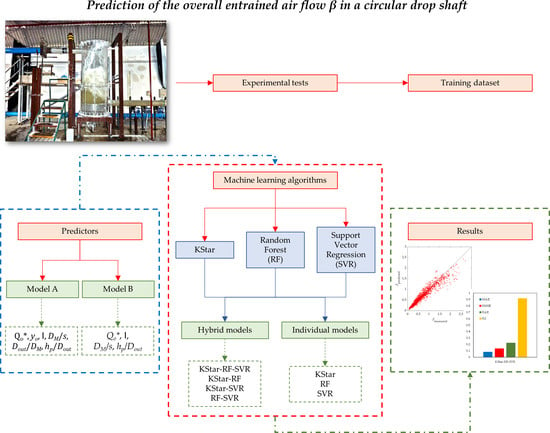
The flowchart of the methodology to develop the proposed individual and hybrid models is shown in Figure 4.
The results of the modeling, in terms of evaluation metrics, are summarized in Table 3 and Figure 5.
Model A showed the best predictive capabilities. The hybrid model Hyb_KStar–RF–SVR (R2 = 0.917, MAE = 0.083, RMSE = 0.136, RAE = 22.47%), which was the most complex hybrid model with three different ML algorithms, led to the best predictions. The hybrid models developed with two ML algorithms showed performances similar to each other and, at the same time, worse than the hybrid model with three ML algorithms. In particular, Hyb_KStar–SVR (R2 = 0.909, MAE = 0.086, RMSE = 0.142, RAE = 23.31%) slightly outperformed both Hyb_KStar–RF (R2 = 0.905, MAE = 0.092, RMSE = 0.146, RAE = 24.68%) and Hyb_RF–SVR (R2 = 0.909, MAE = 0.089, RMSE = 0.143, RAE = 24.03%). Individual ML algorithms led to the less accurate outcomes, with SVR (R2 = 0.888, MAE = 0.098, RMSE = 0.159, RAE = 26.38%), which was the most accurate, and RF (R2 = 0.882, MAE = 0.104, RMSE = 0.163, RAE = 28.03%), which was the least accurate. All variants of Model A showed a slight tendency to underestimate higher β values. Figure 6 shows the predicted versus observed values for Model A.
Model B underperformed Model A in all its variants. Additionally, in this case, the hybrid model Hyb_KStar–RF–SVR (R2 = 0.888, MAE = 0.096, RMSE = 0.158, RAE = 25.92%) led to the most accurate predictions. However, among the hybrid models based on two ML algorithms, Hyb_RF–SVR (R2 = 0.883, MAE = 0.098, RMSE = 0.162, RAE = 26.53%) was the most accurate, and Hyb_KStar–SVR (R2 = 0.854, MAE = 0.105, RMSE = 0.181, RAE = 28.22%) was the least accurate. Moreover, the individual RF algorithm (R2 = 0.875, MAE = 0.108, RMSE = 0.167, RAE = 29.09%) also led to better forecasts in comparison with Hyb_KStar–SVR. RF was little affected by the absence of yo and Dout/DM among the input variables. The worst predictions were achieved with KStar (R2 = 0.799, MAE = 0.127, RMSE = 0.212, RAE = 34.12%). In Figure 7, predicted versus observed values for Model B are shown.
Model B showed a more pronounced tendency to underestimate higher β values than model A. The trend occurred for β greater than 1.5 and even affected the Hyb_KStar–RF–SVR variant. A partial exception was the RF algorithm, where the trend was less marked.
Figure 8 shows the box plots of the relative errors (i.e., the ratio between the absolute error and the measured values). A positive relative error indicates an underestimation of β, and vice versa. The following observations can be highlighted:
The hybrid models were free of bias. In model A, the individual algorithms did not lead to significantly different relative errors;
The Hyb_KStar–RF–SVR variant was characterized by the narrower interquartile range (IQR) and by the lower number of outliers among all variants both for Model A and Model B;
With the same ML algorithm, Model A had slightly narrower interquartile ranges than Model B;
The number of outliers was significantly higher for single ML algorithms, both for Model A and for Model B. Moreover, for the latter, the number of negative outliers clearly prevailed.
An approach based on ML algorithms for the prediction of the airflow rate entrained in a circular drop shaft had already been proposed in [30]. In that previous study, three individual algorithms—M5P, bagging, and random forest—were compared. The latter had clearly outperformed both M5P and bagging; however, the results were unsatisfactory, as evinced also by the evaluation metrics (the value of R2 was 0.793, while MAE, RMSE, and RAE had, respectively, values of 0.1406, 0.2125, and 38.15%, in the case of RF). The models proposed here proved to be much more accurate than the previous ones.
The better predictive ability of the proposed novel models depends on the following factors:
Different choices of predictors: The inclusion of impact number I and the hp/Dout ratio among the input variables proved to be crucial. The I variable allows considering the air entrainment mechanisms linked to the flow regimes, while hp/Dout allows taking into account the obstruction effect to the dragging of air toward the downstream pipe due to the liquid pool at the bottom of the drop shaft, when its height exceeds the diameter of the downstream pipe.
Hybridization of models: The results show clearly that the hybrid models outperformed the individual-based models for the prediction of the overall entrained airflow.
The hybrid models are more and more frequently used due to their high capacity for improving prediction performances. A hybrid machine learning model provides better performance when the individual models are uncorrelated. For instance, it is possible to build different models on different datasets or features: The less correlated the base models are, the better the prediction performance can be achieved. The idea behind using uncorrelated models is that each could address a weakness in the other. They also have different strengths, which, when combined, will result in a better estimator.
4. Conclusions
An accurate prediction of the overall entrained airflow in a circular drop shaft is essential to avoid the poor operating conditions related to an insufficient air inlet from the outside.
In this study, based on a different combination of predictors, two different models were developed to predict the overall entrained airflow. Data were obtained from a previous, extensive experimental campaign. For each model, seven variants were compared. In particular, three variants were based on the individual algorithms: KStar, random forest, and support vector regression. The other four variants were based on hybrid models developed starting from these three individual algorithms.
Model A, which considers predictors including the dimensionless incoming water discharge, the approach flow filling ratio, the impact number, the ratio between the diameter of the drop shaft and the drop height, the ratio between the diameters of the outlet pipe and of the drop shaft, and the ratio between the pool depth and the diameter of the outlet pipe, provided better predictions, compared with Model B. The latter did not consider both filling ratio and the ratio between outlet pipe diameter and manhole diameter, resulting in a sharp reduction in performances, in particular for the models based on individual KStar and SVR algorithms and for the KStar–SVR hybrid model. However, the inclusion of both impact number I and hp/Dout ratio, which allowed considering air entrainment mechanisms and the obstruction effect related to dragging of air, respectively, led to accurate predictions of air demand.
Moreover, hybrid variants based on all three algorithms led to the best results across all models, with the best metrics, narrower interquartile range, and lower number of outliers among all variants.
Future developments of this research will be aimed at the investigation of different hydraulic structures, e.g., vortex drop shaft and stepped spillway.
Author Contributions
Conceptualization, F.G.; methodology, F.G.; software, F.G.; validation, F.G. and F.D.N., formal analysis, F.G. and F.D.N., investigation, F.G. and F.D.N.; resources, F.G.; data curation, F.G. and F.D.N.; writing-original draft preparation, F.G. and F.D.N.; writing-review and editing, F.G. and F.D.N.; supervision, F.G.; project administration, F.G.. All authors have read and agreed to the published version of the manuscript.
Funding
No external funding.
Institutional Review Board Statement
Not applicable.
Informed Consent Statement
Not applicable.
Data Availability Statement
The datasets analyzed during the current study are available from the corresponding author on reasonable request.
Conflicts of Interest
The authors declare no conflict of interest.
List of Symbols
The following symbols are used in this paper:
| a | = | KStar—generic instance |
| b | = | KStar—generic instance |
| b | = | Support vector machine—bias |
| C | = | Support vector machine—constant |
| Din | = | Upstream pipe diameter |
| DM | = | Drop shaft diameter |
| Dout | = | Outlet pipe diameter |
| F | = | Support vector machine—feature space |
| g | = | Gravitational acceleration |
| ho | = | Incoming flow depth |
| hp | = | Pool depth |
| i | = | KStar—absolute difference between first and last instance |
| I | = | Impact number |
| k | = | Support vector machine—kernel function |
| K* | = | KStar—distance in the complexity computation |
| N | = | Random forest—number of units in the node t |
| P* | = | KStar—probability of all paths from instance a to instance b |
| Q | = | Water discharge |
| Qo* | = | Nondimensional water discharge |
| R | = | Random forest—mean square error in the node t |
| S | = | KStar—model parameter |
| s | = | Drop height |
| t | = | Random forest—generic node |
| V | = | Flow velocity |
| w | = | Support vector machine—weight |
| X | = | Support vector machine—space of the input arrays |
| xi | = | Support vector machine—experimental input values |
| yi | = | Random forest—value assumed by the target variable in the i-th unit |
| yi | = | Support vector machine—experimental target values |
| ym | = | Random forest—average value of the target variable in the node t |
| yo | = | Upstream pipe filling ratio |
| ε | = | Support vector machine—maximum deviation from the experimental target values yi |
| σ | = | Support vector machine—PUK parameter from which the peak tailing factor depends |
| ω | = | Support vector machine—PUK parameter from which the peak half-width depends |
| b | = | Dimensionless entrained airflow |
| ξι | = | Support vector machine—slack variable |
References
- Christodoulou, G.C. Drop manholes in supercritical pipelines. J. Irrig. Drain. Eng. 1991, 117, 37–47. [Google Scholar] [CrossRef]
- Rajaratnam, N.; Mainali, A.; Hsung, C.Y. Observations on flow in vertical dropshafts in urban drainage systems. J. Environ. Eng. 1997, 123, 486–491. [Google Scholar] [CrossRef]
- Chanson, H. Hydraulics of rectangular dropshafts. J. Irrig. Drain. Eng. 2004, 130, 523–529. [Google Scholar] [CrossRef] [Green Version]
- Carvalho, R.F.; Leandro, J. Hydraulic characteristics of a drop square manhole with a downstream control gate. J. Irrig. Drain. Eng. 2012, 138, 569–576. [Google Scholar] [CrossRef]
- Granata, F.; de Marinis, G.; Gargano, R. Flow-improving elements in circular drop manholes. J. Hydraul. Res. 2014, 52, 347–355. [Google Scholar] [CrossRef]
- Granata, F. Dropshaft cascades in urban drainage systems. Water Sci. Technol. 2016, 73, 2052–2059. [Google Scholar] [CrossRef]
- Ma, Y.; Zhu, D.Z.; Rajaratnam, N.; van Duin, B. Energy dissipation in circular drop manholes. J. Irrig. Drain. Eng. 2017, 143, 04017047. [Google Scholar] [CrossRef]
- Granata, F.; de Marinis, G.; Gargano, R.; Hager, W.H. Hydraulics of circular drop manholes. J. Irrig. Drain. Eng. 2011, 137, 102–111. [Google Scholar] [CrossRef]
- Granata, F.; de Marinis, G.; Gargano, R. Air-water flows in circular drop manholes. Urban Water J. 2015, 12, 477–487. [Google Scholar] [CrossRef]
- Ma, Y.; Zhu, D.Z.; Rajaratnam, N. Air entrainment in a tall plunging flow dropshaft. J. Hydraul. Eng. 2016, 142, 04016038. [Google Scholar] [CrossRef]
- Azamathulla, H.M.; Haghiabi, A.H.; Parsaie, A. Prediction of side weir discharge coefficient by support vector machine technique. Water Sci. Technol. Water Supply 2016, 16, 1002–1016. [Google Scholar] [CrossRef] [Green Version]
- Roushangar, K.; Khoshkanar, R.; Shiri, J. Predicting trapezoidal and rectangular side weirs discharge coefficient using machine learning methods. ISH J. Hydraul. Eng. 2016, 22, 254–261. [Google Scholar] [CrossRef]
- Azimi, H.; Bonakdari, H.; Ebtehaj, I. Design of radial basis function-based support vector regression in predicting the discharge coefficient of a side weir in a trapezoidal channel. Appl. Water Sci. 2019, 9, 78. [Google Scholar] [CrossRef] [Green Version]
- Granata, F.; Di Nunno, F.; Gargano, R.; de Marinis, G. Equivalent discharge coefficient of side weirs in circular channel—A lazy machine learning approach. Water 2019, 11, 2406. [Google Scholar] [CrossRef] [Green Version]
- Etemad-Shahidi, A.; Yasa, R.; Kazeminezhad, M.H. Prediction of wave-induced scour depth under submarine pipelines using machine learning approach. Appl. Ocean Res. 2011, 33, 54–59. [Google Scholar] [CrossRef] [Green Version]
- Najafzadeh, M.; Azamathulla, H.M. Neuro-fuzzy GMDH to predict the scour pile groups due to waves. J. Comput. Civ. Eng. 2015, 29, 04014068. [Google Scholar] [CrossRef]
- Najafzadeh, M.; Etemad-Shahidi, A.; Lim, S.Y. Scour prediction in long contractions using ANFIS and SVM. Ocean Eng. 2016, 111, 128–135. [Google Scholar] [CrossRef]
- Di Nunno, F.; Alves Pereira, F.; de Marinis, G.; Di Felice, F.; Gargano, R.; Miozzi, M.; Granata, F. Deformation of Air Bubbles Near a Plunging Jet Using a Machine Learning Approach. Appl. Sci. 2020, 10, 3879. [Google Scholar] [CrossRef]
- Zhang, Y.; Azman, A.N.; Xu, K.W.; Kang, C.; Kim, H.B. Two-phase flow regime identification based on the liquid-phase velocity information and machine learning. Exp. Fluids 2020, 61, 1–16. [Google Scholar] [CrossRef]
- Sujjaviriyasup, T.; Pitiruek, K. Hybrid ARIMA-Support Vector Machine Model for Agricultural Production Planning. Appl. Math. Sci. 2013, 7, 2833–2840. [Google Scholar] [CrossRef]
- Gala, Y.; Fernández, A.; Díaz, J.; Dorronsoro, J.R. Hybrid machine learning forecasting of solar radiation values. Neurocomputing 2016, 176, 48–59. [Google Scholar] [CrossRef]
- Khozani, Z.S.; Khosravi, K.; Pham, B.T.; Kløve, B.; Mohtar, W.H.M.W.; Yaseen, Z.M. Determination of compound channel apparent shear stress: Application of novel data mining models. J. Hydroinform. 2019, 21, 798–811. [Google Scholar] [CrossRef] [Green Version]
- Kombo, O.H.; Kumaran, S.; Sheikh, Y.H.; Bovim, A.; Jayavel, K. Long-Term Groundwater Level Prediction Model Based on Hybrid KNN-RF Technique. Hydrology 2020, 7, 59. [Google Scholar] [CrossRef]
- Breiman, L. Random Forests. Mach. Learn. 2001, 45, 5–32. [Google Scholar] [CrossRef] [Green Version]
- Breiman, L.; Friedman, J.H.; Olshen, R.A.; Stone, C.J. Classification and Regression Trees; CRC Press: Boca Raton, FL, USA, 2011. [Google Scholar]
- Cortes, C.; Vapnik, V. Support-vector networks. Mach. Learn. 1995, 20, 273–297. [Google Scholar] [CrossRef]
- Cleary, J.G.; Trigg, L.E. K*: An instance-based learner using an entropic distance measure. In Machine Learning Proceedings 1995; Morgan Kaufmann: San Francisco, CA, USA, 1995; pp. 108–114. [Google Scholar]
- Kittler JHatef, M.; Duin, R.P.W.; Matas, J. On Combining Classifiers. IEEE Trans. Pattern Anal. Mach. Intell. 1998, 20, 226–239. [Google Scholar] [CrossRef] [Green Version]
- Quinlan, J.R. Learning with continuous classes. In Proceedings of the 5th Australian Joint Conference on Artificial Intelligence, Hobart, Australia, 16–18 November 1992; Volume 92, pp. 343–348. [Google Scholar]
- Granata, F.; de Marinis, G. Machine learning methods for wastewater hydraulics. Flow Meas. Instrum. 2017, 57, 1–9. [Google Scholar] [CrossRef]
Figure 1.
The experimental model: (a) image of Model 1, with clearly visible air entrainment phenomena; (b) sketch of the model with indicated symbols.
Figure 1.
The experimental model: (a) image of Model 1, with clearly visible air entrainment phenomena; (b) sketch of the model with indicated symbols.

Figure 2.
Typical architecture of the random forest algorithm.

Figure 3.
Typical architecture of the support vector regression algorithm.

Figure 4.
Flowchart of the model development procedure.

Figure 5.
Error histograms (left) and coefficients of determination (right).

Figure 6.
Model A: bpredicted versus bmeasured.


Figure 7.
Model B: βpredicted versus βmeasured.


Figure 8.
Box plots of the relative errors: (a) Model A and (b) Model B.


Table 1.
Evaluation metrics.
| Coefficient of Determination: it represents a measure of the model accuracy, assessing how well the model fits the experimental results. | |
| Mean Absolute Error: it provides the average error magnitude for the predicted values. | |
| Root-Mean-Squared Error: it provides the square root of the average squared errors for the predicted values. It has the benefit of penalizing large errors. | |
| Relative Absolute Error: it provides the normalized total absolute error with respect to the sum of the difference between the mean and each measured value. | |
| In the above formulas, m is the total number of experimental data, fi is the predicted value for the i-th data point, yi is the measured value for the i-th data point, ya is the averaged value of the experimental data. | |
Table 2.
Statistical description of the training dataset, with the exclusion of Dout/DM.
| Qo* | yo | I | DM/s | hp/Dout | b | |
|---|---|---|---|---|---|---|
| Minimum Value | 0.027 | 0.158 | 0.234 | 0.167 | 0.258 | 0.029 |
| First Quartile | 0.135 | 0.295 | 0.728 | 0.320 | 0.639 | 0.349 |
| Median | 0.294 | 0.385 | 0.998 | 0.480 | 0.985 | 0.573 |
| Third Quartile | 0.507 | 0.503 | 1.607 | 0.667 | 1.636 | 0.930 |
| Maximum Value | 1.417 | 0.950 | 6.374 | 2.000 | 4.600 | 2.709 |
| Mean | 0.352 | 0.406 | 1.309 | 0.578 | 1.199 | 0.694 |
| Standard Deviation | 0.265 | 0.139 | 0.895 | 0.401 | 0.725 | 0.473 |
| Skewness | 0.657 | 0.444 | 1.043 | 0.730 | 0.885 | 0.770 |
Table 3.
Prediction models and variants, with the relevant predictors and evaluation metrics.
| Model | Predictors | Algorithm | R2 | MAE | RMSE | RAE (%) |
|---|---|---|---|---|---|---|
| A | Qo*, yo, I, DM/s, Dout/DM, hp/Dout | Hyb_KStar–RF–SVR | 0.917 | 0.083 | 0.136 | 22.47 |
| Hyb_KStar–RF | 0.905 | 0.092 | 0.146 | 24.68 | ||
| Hyb_KStar–SVR | 0.909 | 0.086 | 0.142 | 23.31 | ||
| Hyb_RF–SVR | 0.909 | 0.089 | 0.143 | 24.03 | ||
| KStar | 0.887 | 0.099 | 0.159 | 26.59 | ||
| RF | 0.882 | 0.104 | 0.163 | 28.03 | ||
| SVR | 0.888 | 0.098 | 0.159 | 26.38 | ||
| B | Qo*, I, DM/s, hp/Dout | Hyb_KStar–RF–SVR | 0.888 | 0.096 | 0.158 | 25.92 |
| Hyb_KStar–RF | 0.877 | 0.102 | 0.166 | 27.58 | ||
| Hyb_KStar–SVR | 0.854 | 0.105 | 0.181 | 28.22 | ||
| Hyb_RF–SVR | 0.883 | 0.098 | 0.162 | 26.53 | ||
| KStar | 0.799 | 0.127 | 0.212 | 34.21 | ||
| RF | 0.875 | 0.108 | 0.167 | 29.09 | ||
| SVR | 0.818 | 0.121 | 0.202 | 32.58 |
Publisher’s Note: MDPI stays neutral with regard to jurisdictional claims in published maps and institutional affiliations. |
© 2022 by the authors. Licensee MDPI, Basel, Switzerland. This article is an open access article distributed under the terms and conditions of the Creative Commons Attribution (CC BY) license (https://creativecommons.org/licenses/by/4.0/).
Share and Cite
MDPI and ACS Style
Granata, F.; Di Nunno, F. Air Entrainment in Drop Shafts: A Novel Approach Based on Machine Learning Algorithms and Hybrid Models. Fluids 2022, 7, 20. https://doi.org/10.3390/fluids7010020
AMA Style
Granata F, Di Nunno F. Air Entrainment in Drop Shafts: A Novel Approach Based on Machine Learning Algorithms and Hybrid Models. Fluids. 2022; 7(1):20. https://doi.org/10.3390/fluids7010020
Chicago/Turabian StyleGranata, Francesco, and Fabio Di Nunno. 2022. "Air Entrainment in Drop Shafts: A Novel Approach Based on Machine Learning Algorithms and Hybrid Models" Fluids 7, no. 1: 20. https://doi.org/10.3390/fluids7010020