Mathematical Model for Axisymmetric Taylor Flows Inside a Drop


1
Faculty of Control Systems and Robotics, Saint Petersburg National Research University of Information Technologies, Mechanics and Optics (ITMO University), Kronverkskiy, 49, 197101 Saint Petersburg, Russia
2
Department of Optimization of Chemical and Biotechnological Equipment, Saint Petersburg State Institute of Technology (Technical University), Moscovskiy Prospect, 26, 190013 Saint Petersburg, Russia
*
Author to whom correspondence should be addressed.
Fluids 2021, 6(1), 7; https://doi.org/10.3390/fluids6010007
Submission received: 2 December 2020
/
Revised: 21 December 2020
/
Accepted: 24 December 2020
/
Published: 26 December 2020
(This article belongs to the Special Issue Flow and Heat Transfer Intensification in Chemical Engineering)
Abstract
:Analytical solutions of the Stokes equations written as a differential equation for the Stokes stream function were obtained. These solutions describe three-dimensional axisymmetric flows of a viscous liquid inside a drop that has the shape of a spheroid of rotation and have a similar set of characteristics with Taylor flows inside bubbles that occur during the transfer of a two-component mixture through tubes.
1. Introduction
The Taylor flow regime is the most favorable of the known regimes for microchannels, since it provides, on the one hand, an intensification of mass transfer due to Taylor vortices, and on the other hand, a sufficient residence time, in view of the rather moderate velocities of phase motion (typically 0.01–0.1 m/s, and not larger than 0.8–1 m/s), which are typical for this regime [1,2]. The velocity of bubbles or droplets is characterized by capillary number Ca = μU/σ where μ is a liquid viscosity, U is adispersed phase (bubbles or droplets) velocity and σ is an interfacial tension. Usually Ca number does not exceed 0.01–0.1, and the Reynolds number for the flows in micro and mini-channels is less than 2000, corresponding thus to the laminar flow [3]. These features make it possible to achieve a high mixing intensity without significantly complicating the equipment and generate great interest in this type of flow.
In the last two to three decades, many papers were devoted to both the hydrodynamics of the Taylor flow and mass transfer in it [4,5,6,7,8,9,10]. Most of these works in fluid dynamics are based on experimental or numerical experiments. At the same time, it is important to search for independent theoretical methods that allow one to obtain a general a priori idea of the dispersed flow inside droplets or bubbles, including the shape of streamlines.
Such two-component liquid streams belong to the class of Taylor streams and are widely used in various industries [1,2].
One of the first models describing the motion of Taylor bubbles in channels was published by F. Bretherton [11]. The extended Bretherton model for Taylor bubbles at moderate capillary numbers was proposed by E. Klaseboer [12].
A number of works [13,14,15,16] were devoted to the study of Taylor flows. In [17], the method of micro Particle Image Velocimetry is used to study Taylor vortices inside an elongated bubble. In [18] the circulation patterns within the dispersed phase for regular Taylor two-phase flows were constructed using the FEATFLOW program.
It is worth noting that the actual shape of the Taylor bubbles may be far from the ideal geometric shape. Nevertheless, modeling, which considers the Taylor flow in a domain with an idealized form, is used in a number of studies [19]. In [20,21], the shape of the bubbles is approximated by a part of a cylinder with hemispherical caps or a prolate ellipsoid at ends.
In the type of flow that we are considering, a mixture of two liquids that have different viscosity coefficients is transferred through the channel and one liquid is distributed in the form of bubbles inside the other one (Figure 1). The liquid interacting with the channel walls moves along its axis and drives the gas bubbles or the droplets of the second liquid. At a constant two-phase velocity of a mixture of liquids through the channel, this flow can be considered stationary and axisymmetric (for the case when the capillary forces dominate over gravitational forces, i.e., for liquids similar to the water at the channel diameter smaller than ≈ 3 mm).
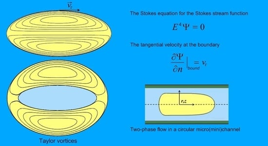
Due to the presence of friction force at the boundary of two fluids and friction between the fluid and the channel walls, a vortex flow occurs in the inner part of the bubbles during the movement of the mixture through the channel (Figure 2).
In our previous work [22], we obtained solutions for two-dimensional flows inside an elliptical region, which demonstrated the presence of both the main toroidal vortex (similar to that shown in Figure 2) and two satellite vortices. These solutions generally reflect the nature of the droplet/bubble flows in the Taylor two-phase flow.
The system of Stokes equations is often used in mathematical models to describe the flow of a liquid with a set of characteristics similar to the Taylor flows described above. It should be noted that in most problems, the system of Stokes equations can be solved only numerically, and analytical solutions of Stokes equations have been found only for a small class of problems with a specific regular boundary shape [23,24]. In the presence of curvilinear sections of the boundary in some problems, it turns out to be expedient to use the corresponding curvilinear coordinate system. In [25], solutions were found for a circular cavity in a polar coordinate system; in [26], solutions of the Stokes equations were obtained in an elliptic coordinate system for a region bounded by two confocal ellipses. Solutions of the Stokes equations for two-dimensional flows inside an elliptic region were considered in article [22]. A similar approach is used for three-dimensional flows in cases where the boundary has a spherical or cylindrical shape [27,28].
The purpose of this work is to obtain analytical solutions of the Stokes equations for a mathematical model that describes the three-dimensional Taylor flow inside an elongated bubble (Figure 2). In the considered simplification of the physical model, the bubble shape is specified as the surface of a spheroid (ellipsoid of revolution), and the fluid flow inside the bubble is assumed to be axisymmetric. Thus, in comparison with work [22], in this article we simulate the flow for three-dimensional shape of the bubble boundary. Another form of boundary geometry leads to the emergence of a more complex axisymmetric pressure field inside the bubble and becomes a more accurate approximation of the real physical model.
The obtained analytical solutions of the Stokes equations make it possible to qualitatively compare the flow pattern inside the bubbles with experimental data and the results of numerical modeling for Taylor flows, and can also be used as a benchmark to assess the quality of numerical algorithms [29,30].
2. Problem Formulation
We are considering a three-dimensional axisymmetric Stokes flow in the region bounded by a spheroid (Figure 3). We assume that the boundary of the spheroid is impenetrable and the shape of the spheroid does not change over time. The fluid flow inside the spheroid is caused by the motion of the boundary, in which the velocity of the points on the boundary is directed tangentially to the boundary of the spheroid. In this problem, we will assume that the velocity vector at the boundary of the spheroid lies in the plane passing through the axis of symmetry of the spheroid.
The described type of flow inside the spheroid has a similar set of characteristics with Taylor flows inside bubbles (Figure 2) and represents their simplified mathematical model.
Let us consider the derivation of solutions to the Stokes equations that describe fluid flows for a given system. We introduce a cylindrical coordinate system centered at a point that halves the segment lying between the foci of the spheroid (Figure 3). Since the flow is axisymmetric, we can write equations in two coordinates . A cross section of a spheroid is shown in Figure 4. The axis divides the border of the ellipse into two parts, and . We assume that the distribution that defines the velocity at the boundary of the spheroid has the same form on any half and an ellipse (, ) in any plane passing through the axis .
The condition specifying the tangential velocity at the boundary will be written as:
The radial component of the velocity on the axis of symmetry of the spheroid equals to zero:
In the process of describing the fluid flow and constructing the solution of the Stokes equations in this work, we will use the Stokes stream function (it is necessary to distinguish this function from the stream function used in hydrodynamics to describe two-dimensional flows). Velocity components are related to the Stokes stream function by the following relations [23]:
Let us formulate the boundary conditions for the Stokes stream function. Equation (2) will be written in the form:
The normal component of the velocity at the ellipse boundary is equals to zero, therefore:
The condition for the tangential velocity (1) at the boundary of the ellipse takes the form:
Taking into account the specific shape of the domain boundary, the solution of Stokes equations in elliptic coordinates was derived:
—focal length.
The Lame coefficients in elliptic coordinates are:
The Stokes equation for the Stokes stream function are written as [31]:
where the operator has the form:
Taking into account relation between coordinates , we get:
It should be noted that Equation (6) differs from the classical biharmonic equation for the two-dimensional stream function [26]: Formula (8) includes the last two terms containing the hyperbolic cotangent and the cotangent, which are absent in the formula for the Laplace operator in elliptic coordinates.
In elliptical coordinates, the halves of the ellipse (Figure 4) will transform into two rectangles, given by the inequalities: , and , (Figure 5). The segment between the foci will correspond to the segments , , . Parts of boundary , will transform to segments , , . The segments between the foci and points , will be segments , , .
Let us formulate the boundary conditions for the Stokes stream function in elliptic coordinates. Condition (4) will be written as:
Condition (3) takes the form:
We write the boundary condition for the tangential velocity (5) on the right half of the ellipse in the form:
Further, we assume that the velocity at the boundary of the ellipse is symmetric about the axis .
3. Problem Solution
In the process of constructing a solution of Equation (6), we perform the following replacement:
This replacement makes it possible to significantly simplify Formula (8) for the differential operator:
We will seek a solution in the form:
Integration of corresponding differential equations, gives us:
In elliptical coordinates, the stream function takes the form:
A detailed derivation of Formula (15) is given in the Appendix A.
It is worth noting that a similar technique for constructing solutions was previously used to describe the flow outside a solid body in the form of a spheroid during its motion in a viscous fluid [31].
To complete the process of constructing the Stokes stream function defining the fluid flow inside the bubble we need to find the coefficients , , in the expression (16) that satisfy the boundary conditions.
Due to the peculiarity of constructing the stream function in the form (16), boundary condition (10) will be satisfied automatically.
From the condition on the segment between the foci of the ellipse (11), we obtain linear equations for the coefficients:
From condition (9) we get:
where , the value defines the boundary of the spheroid.
Equations (17) and (18) define two linear equations for three unknown constants. Thus, one of the constants , , remains free, which makes it possible to vary the velocity of the border.
It should be noted that due to axial symmetry, the problem of constructing a solution inside an ellipse is reduced to the problem of constructing a solution in its half. Due to the peculiarity of the elliptical coordinate system, the Stokes stream functions given in different halves of the ellipse (Figure 4) will be symmetric about the axis (functions for different parts will have the same modulus and the opposite sign). This will ensure the fulfillment of the boundary conditions and the continuity condition of the stream function and its derivatives on the axis .
4. Results and Discussion
The obtained analytical solution (16) opens up an opportunity for modeling of fluid flow inside the spheroid. It is worth noting that functions of the form (16) impose specific restrictions on the velocity function at the boundary. Due to the presence of the sine of the coordinate in Formula (16), the flow velocity function tends to zero at the ends of the ellipse and increases at its middle part. However, this feature is natural for the Taylor flows.
Let us consider an example of such a flow, given by an analytical stream function for a certain choice of constants in Formula (16). Velocity function at the boundary is shown in Figure 6. Flow streamlines are shown in Figure 7. Streamlinesin this example correspond to the following coefficients in (16): , , .
A flow with a similar set of parameters can be observed in the by-pass flow mode in microchannels, as well as inside a bubble moving far from the channel walls. In this type of flow, streamlines are around the bubble and are not closed, as shown in Figure 2. This feature of the flow leads to the appearance of shear stresses at the interface between liquids, acting from the nose of the bubble to its tail [32,33], which create circulation inside the bubble (Figure 7).
The analytical solution (16) can be used to simulate a three-dimensional axisymmetric flow between two confocal spheroids. In this case, the normal velocity at the boundary of the inner spheroid should be equal to zero. Condition (17) must be replaced by a condition that ensures the equality of the stream function to zero at the boundary of the inner spheroid:
where , the value defines the boundary of the inner spheroid.
Figure 8 shows the streamlines for the flow between two spheroids. The velocity function at the boundary of the spheroids is shown in Figure 9. The upper function (highlighted in blue) corresponds to the velocity on the outer spheroid, the bottom function (highlighted in red) corresponds to the velocity on the inner spheroid. Figures from this example correspond to the following coefficients in (16): , , .
It should be noted that a similar problem of the Stokes flow between two cylinders with an elliptical profile was previously considered in [26].
5. Conclusions
The geometric shape of the Taylor bubble can naturally be approximated by a spheroid of revolution. Therefore, a comparison of Taylor flows with axisymmetric Stokes flows inside a spheroid is quite applicable, despite the fact that the actual shape of the bubble can be more complicated due to the presence of microwaves on its surface.
This work is devoted to the derivation of exact analytical solutions of the Stokes equations for the model of axisymmetric flows inside the Taylor bubble. These solutions can be used as a tool for assessment of the numerical algorithms quality by comparing the result of the numerical algorithm with exact analytical solution. The advantage of this evaluation method is that it excludes the possibility of error accumulation which can occur in the case of comparing numerical algorithms with each other.
Author Contributions
Conceptualization, R.S.A. and I.Y.P.; Formal analysis, I.V.M. and R.S.A.; Methodology, I.Y.P.; Supervision, I.V.M.; Writing—original draft, I.V.M.; Writing—review & editing, R.S.A. and I.Y.P. All authors have read and agreed to the published version of the manuscript.
Funding
This research received no external funding.
Conflicts of Interest
The authors declare no conflict of interest.
Appendix A. Derivation of a Stokes Stream Function
Let us consider the derivation of the solution for Equation (6).
Substitution of expression (14) into Equation (13), gives us:
Let us introduce the function:
For function we get the following expression:
It is worth noting that the term in square brackets must equals to zero to execute the Equation (6). Since is a function of a variable , this implies
The solution of this system is a function:
Substituting this function in (A2), we obtain the inhomogeneous equation:
Particular solution of this equation is a function of the following form:
Another part of the solution will correspond to the solution of the following homogeneous equation:
Integration gives us:
By integrating this equation, we get:
The general solution to Equation (A6) takes the form:
For a stream function satisfying Equation (6), we obtain the following expression:
References
- Kreutzer, M.T.; Kapteijn, F.; Moulijn, J.A.; Heiszwolf, J.J. Multiphase monolith reactors: Chemical reaction engineering of segmented flow in microchannels. Chem. Eng. Sci. 2005, 60, 5895–5916. [Google Scholar] [CrossRef]
- Bauer, T.; Schubert, M.; Lange, R.; Abiev, R.S. Intensification of heterogeneous catalytic gas-fluid interactions in reactors with a multichannel monolithic catalyst. Russ. J. Appl. Chem. 2006, 79, 1047–1056. [Google Scholar] [CrossRef]
- Liu, H.; Vandu, C.O.; Krishna, R. Hydrodynamics of Taylor Flow in Vertical Capillaries: FlowRegimes, Bubble Rise Velocity, Liquid Slug Length, and Pressure Drop. Ind. Eng. Chem. Res. 2005, 44, 4884–4897. [Google Scholar] [CrossRef]
- Ghaini, A.; Kashid, M.N.; Agar, D.W. Effective interfacial area for mass transfer in the liquid–liquid slug flow capillary microreactors. Chem. Eng. Process. Process Intensif. 2010, 49, 358–366. [Google Scholar] [CrossRef]
- Abiev, R.S. Gas-liquid and gas-liquid-solid mass transfer model for Taylor flow in micro (milli) channels: A theoretical approach and experimental proof. Chem. Eng. J. Adv. 2020, 4, 100065. [Google Scholar] [CrossRef]
- Shao, N.; Gavriilidis, A.; Angeli, P. Mass transfer during Taylor flow in microchannels with and withoutchemical reaction. Chem. Eng. J. 2010, 160, 873–881. [Google Scholar] [CrossRef]
- Abiev, R.S.; Butler, C.; Cid, E.; Lalanne, B.; Billet, A.-M. Mass transfer characteristics and concentration field evolution for gas-liquid Taylor flow in milli channels. Chem. Eng. Sci. 2019, 207, 1331–1340. [Google Scholar] [CrossRef] [Green Version]
- Butler, C.; Cid, E.; Billet, A.-M. Modelling of mass transfer in Taylor flow: Investigation with the PLIF-I technique. Chem. Eng. Res. Des. 2016, 115, 292–302. [Google Scholar] [CrossRef] [Green Version]
- Butler, C.; Lalanne, B.; Sandmann, K.; Cid, E.; Billet, A.-M. Mass transfer in Taylor flow: Transfer rate modelling from measurements at the slug and filmscale. Int. J. Multiph. Flow 2018, 105, 185–201. [Google Scholar] [CrossRef] [Green Version]
- Dietrich, N.; Loubière, K.; Jimenez, M.; Hébrard, G.; Gourdon, C. A new directtechnique for visualizing and measuring gas–liquid mass transfer aroundbubbles moving in a straight millimetric square channel. Chem. Eng. Sci. 2013, 100, 172–182. [Google Scholar] [CrossRef] [Green Version]
- Bretherton, F.P. The motion of long bubbles in tubes. J. Fluid Mech. 1961, 10, 166–188. [Google Scholar] [CrossRef]
- Klaseboer, E.; Gupta, R.; Manica, R. An extended Bretherton model for long Taylor bubbles at moderate capillary numbers. Phys. Fluids 2014, 26, 032107. [Google Scholar] [CrossRef]
- Falconi, C.J.; Lehrenfeld, C.; Marschall, H.; Meyer, C.; Abiev, R.S.; Bothe, D.; Reusken, A.; Schluter, M.; Wörner, M. Numerical and experimental analysis of local flow phenomena in laminar Taylor flow in a square mini-channel. Phys. Fluids 2016, 28, 012109. [Google Scholar] [CrossRef]
- Dore, V.; Tsaoulidis, D.; Angeli, P. Mixing patterns in water plugs during water/ionic liquid segmented flow in microchannels. Chem. Eng. Sci. 2012, 80, 334–341. [Google Scholar] [CrossRef] [Green Version]
- Li, Q.; Angeli, P. Experimental and numerical hydrodynamic studies of ionic liquid-aqueous plug flow in small channels. Chem. Eng. J. 2017, 15, 17–736. [Google Scholar] [CrossRef]
- Marschall, H.; Falconi, C.; Lehrenfeld, C.; Abiev, R.; Wörner, M.; Reusken, A.; Bothe, D. Transport Processes at Fluidic Interfaces. In Direct Numerical Simulations of Taylor Bubbles in a Square Mini-Channel: Detailed Shape and Flow Analysis with Experimental Validation; Springer: Berlin/Heidelberg, Germany, 2017; pp. 663–679. [Google Scholar] [CrossRef]
- Meyer, C.; Hoffmann, M.; Schlüter, M. Micro-PIV analysis of gas–liquid Taylor flow in a vertical oriented square shaped fluidic channel. Int. J. Multiph. Flow 2014, 67, 140–148. [Google Scholar] [CrossRef]
- Kashid, M.; Platte, F.; Agar, D.; Turek, S. Computational modelling of slug flow in a capillary microreactor. J. Comput. Appl. Math. 2007, 203, 487–497. [Google Scholar] [CrossRef] [Green Version]
- Kashid, M.N.; Fernandez Rivas, D.; Agar, D.W.; Turek, S. On the hydrodynamics of liquid–liquid slug flow capillary microreactors. Asia-Pac. J. Chem. Eng. 2008, 3, 151–160. [Google Scholar] [CrossRef]
- Cherukumudi, A.; Klaseboer, E.; Khan, S.A.; Manica, R. Prediction of the shape and pressure drop of Taylor bubbles in circular tubes. Microfluid. Nanofluidics 2015, 19, 1221–1233. [Google Scholar] [CrossRef]
- Abiev, R.S. Analysis of local pressure gradient inversion and form of bubbles in Taylor flow in microchannels. Chem. Eng. Sci. 2017, 174, 403–412. [Google Scholar] [CrossRef]
- Makeev, I.V.; Popov, I.Y.; Abiev, R.S. Analytical solution of Taylor circulation in a prolate ellipsoid droplet in the frame of 2D Stokes equations. Chem. Eng. Sci. 2019, 207, 145–152. [Google Scholar] [CrossRef]
- Van Der Woude, D.; Clercx, H.J.H.; Van Heijst, G.J.F.; Meleshko, V.V. Stokes flow in a rectangular cavity by rotlet forcing. Phys. Fluids 2007, 19, 083602. [Google Scholar] [CrossRef]
- Gürcan, F.; Gaskell, P.H.; Savage, M.D.; Wilson, M. Eddy genesis and transformation of Stokes flow in a double-lid driven cavity. Proc. Inst. Mech. Eng. Part C J. Mech. Eng. Sci. 2003, 217, 353–364. [Google Scholar] [CrossRef]
- Krasnopolskaya, T.S.; Meleshko, V.; Peters, G.; Meijer, H.E.H. Steady stokes flow in an annular cavity. Q. J. Mech. Appl. Math. 1996, 49, 593–619. [Google Scholar] [CrossRef]
- Saatdjian, E.; Midoux, N.; Andreé, J.C. On the solution of Stokes’ equations between confocal ellipses. Phys. Fluids 1994, 6, 3833–3846. [Google Scholar] [CrossRef]
- Tosi, N.; Martinec, Z.; Brajanovski, M.; Müller, T.M.; Gurevich, B. Semi-analytical solution for viscous Stokes flow in two eccentrically nested spheres. Geophys. J. Int. 2007, 170, 1015–1030. [Google Scholar] [CrossRef] [Green Version]
- Smolkina, M.O.; Popov, I.Y.; Blinova, I.V.; Milakis, E. On the metric graph model for flows in tubular nanostructures. Nanosyst. Phys. Chem. Math. 2019, 10, 6–11. [Google Scholar] [CrossRef] [Green Version]
- Popov, I.Y.; Lobanov, I.S.; Popov, S.I.; Popov, A.I.; Gerya, T.V. Practical analytical solutions for benchmarking of 2-D and 3-D geodynamic Stokes problems with variable viscosity. Solid Earth 2014, 5, 461–476. [Google Scholar] [CrossRef] [Green Version]
- Driesen, C.H.; Kuerten, J. An accurate boundary-element method for Stokes flow in partially covered cavities. Comput. Mech. 2000, 25, 501–513. [Google Scholar] [CrossRef]
- Happel, J.; Brenner, H. Low Reynolds Number Hydrodynamics: With Special Applications to Particulate Media; Prentice-Hall: Upper Saddle River, NJ, USA, 1965; p. 553. [Google Scholar]
- Abiev, R.S. Simulation of the slug flow of a gas-liquid system in capillaries. Theor. Found. Chem. Eng. 2008, 42, 105–117. [Google Scholar] [CrossRef]
- Abiev, R.S. Circulation and bypass modes of the slug flow of a gas-liquid mixture in capillaries. Theor. Found. Chem. Eng. 2009, 43, 298–306. [Google Scholar] [CrossRef]
Figure 1.
Two-component liquid in circular channel (r,z).

Figure 2.
Streamlines in the elongated bubble. Arrows characterize the velocity vectorsin the frame of the moving bubble. Reproduced from [14] with permission of Elsevier.
Figure 2.
Streamlines in the elongated bubble. Arrows characterize the velocity vectorsin the frame of the moving bubble. Reproduced from [14] with permission of Elsevier.

Figure 3.
Spheroid. The velocity vector at the boundary is shown in blue.

Figure 4.
Cross section of a spheroid in the axial plane.

Figure 5.
Domain in elliptical coordinates.

Figure 6.
Velocity function at S1.

Figure 7.
Picture of the streamlines in the ellipsoide. Results of calculations.

Figure 8.
Picture of the streamlines in the volume between outer and inner coaxial ellipsoids. Results of calculations.
Figure 8.
Picture of the streamlines in the volume between outer and inner coaxial ellipsoids. Results of calculations.

Figure 9.
Velocity function at S1 for outer and inner spheroids.

Publisher’s Note: MDPI stays neutral with regard to jurisdictional claims in published maps and institutional affiliations. |
© 2020 by the authors. Licensee MDPI, Basel, Switzerland. This article is an open access article distributed under the terms and conditions of the Creative Commons Attribution (CC BY) license (http://creativecommons.org/licenses/by/4.0/).
Share and Cite
MDPI and ACS Style
Makeev, I.V.; Abiev, R.S.; Popov, I.Y. Mathematical Model for Axisymmetric Taylor Flows Inside a Drop. Fluids 2021, 6, 7. https://doi.org/10.3390/fluids6010007
AMA Style
Makeev IV, Abiev RS, Popov IY. Mathematical Model for Axisymmetric Taylor Flows Inside a Drop. Fluids. 2021; 6(1):7. https://doi.org/10.3390/fluids6010007
Chicago/Turabian StyleMakeev, Ilya V., Rufat Sh. Abiev, and Igor Yu. Popov. 2021. "Mathematical Model for Axisymmetric Taylor Flows Inside a Drop" Fluids 6, no. 1: 7. https://doi.org/10.3390/fluids6010007