Coating Flow Near Channel Exit. A Theoretical Perspective

Department of Mechanical and Materials Engineering, University of Western Ontario, London, ON N6A 5B9, Canada
*
Author to whom correspondence should be addressed.
Fluids 2020, 5(4), 180; https://doi.org/10.3390/fluids5040180
Submission received: 13 September 2020
/
Revised: 4 October 2020
/
Accepted: 9 October 2020
/
Published: 15 October 2020
(This article belongs to the Special Issue Thermal Flows)
Abstract
:The planar flow of a steady moving-wall free-surface jet is examined theoretically for moderate inertia and surface tension. The method of matched asymptotic expansion and singular perturbation is used to explore the rich dynamics near the stress singularity. A thin-film approach is also proposed to capture the flow further downstream where the flow becomes of the boundary-layer type. We exploit the similarity character of the flow to circumvent the presence of the singularity. The study is of close relevance to slot and blade coating. The jet is found to always contract near the channel exit, but presents a mild expansion further downstream for a thick coating film. We predict that separation occurs upstream of the exit for slot coating, essentially for any coating thickness near the moving substrate, and for a thin film near the die. For capillary number of order one, the jet profile is not affected by surface tension but the normal stress along the free surface exhibits a maximum that strengthens with surface tension. In contrast to existing numerical findings, we predict the existence of upstream influence as indicated by the nonlinear pressure dependence on upstream distance and the pressure undershoot (overshoot) in blade (slot) coating at the exit.
1. Introduction
We examine the free-surface flow of a planar moving-wall jet at moderate Reynolds and capillary numbers near and far from the channel exit as encountered in coating flow. With the advent of high-speed coating and the use of low-viscosity liquids, inertia is becoming increasingly important but has been traditionally neglected in the modelling of coating flow. General aspects on the classification and analyses of coating flows can be found in the reviews by Ruschak [1] and Weinstein and Ruschak [2]. The current work focuses on slot and blade coating flows which, in addition to the substrate movement, typically involve an adverse or a favorable pressure gradient.
In slot coating, the liquid is forced into the slot die, and distributes through the narrow slot before it emerges onto the moving substrate. A low-pressure area or vacuum is imposed upstream of the die to facilitate a faster and more stable coating process. Consequently, part of the flow is driven downstream by the moving substrate and part of it circulates upstream in the low-pressure area, which causes a streamwise adverse pressure gradient to act inside the channel formed between the downstream die and the moving substrate. In blade coating, the flow lies between a fixed blade of a prescribed shape and a substrate moving parallel to itself. The coating liquid is dragged inside the channel by the moving substrate, which causes a hydrodynamic pressure rise at the upstream of the blade. The pressure rise causes the blade to reject most of the liquid, and only a fraction passes into the narrow channel. Since the drag flow can only carry half of the coating liquid, a streamwise favorable pressure gradient is generated to carry the rest [3]. In this case, the pressure gradient forces the coating liquid in the same direction as the movement of the substrate inside the channel. In both slot and blade coating, the moving substrate drags the flow out of the channel in the form of a free-surface wall jet, and a thin layer of liquid film is obtained. In the present work, only the pressure gradient immediately upstream of the blade or die exit is accounted for, which is found in reality to be very close to constant. Consequently, the flow inside the channel will be assumed to be a superposition of Couette (velocity driven) and Poiseuille (pressure driven) flows.
Aside from its industrial importance, coating flow is fundamentally important as it spans various flow regimes. In an effort to clearly identify these regimes, de Ryck and Quere [4] carried out different experiments on fibre coating and used dimensional arguments, which illustrate the situation of coating flow in general. The visco-capillary range corresponds to slow coating flow and negligible Weber number, obeying the well-known Landau equation [5]. In this case, the film thickness results from a balance between capillarity and viscous forces. For coating flow of liquids of low viscosity (such as water) at higher velocity (about 1 m/s), the measurements of de Ryck and Quere were shown to deviate considerably from the Landau law, even if the capillary number remained negligible (Ca < 0.05). This is the visco-inertial regime, corresponding to a Weber number of order 1. At larger velocities (We > 1), the coating flow does not seem to depend any longer on the surface tension. This observation corroborates well findings for coating flow in general, as the thickness measurements reported by Lee et al. [6] and Becker and Wang [7] indicate for slot coating. De Ryck and Quere [4] also point out that the boundary-layer regime should be relevant to most industrial fibre-coating processes. Similarly, the more recent thickness measurements of Chang et al. [8] for low-viscosity slot-coating films show that viscous and surface tension effects become important only below a critical Reynolds number. At low speed, the minimum wet thickness increases with increasing capillary number but becomes independent of the capillary number for Ca > 0.3. Above the critical Reynolds number, fluid inertia becomes dominant. In this region, the minimum wet thickness decreases as the Reynolds number increases. Chang et al. [8] also established that inertial forces cannot be neglected in slot coating for Re larger than 10, which roughly corresponds to a substrate speed of 1 m/s. The earlier measurements of Carvalho and Kheshgi [9] show that the visco-capillary model remains valid at capillary numbers below unity. Their measurements also indicate that the model becomes less and less useful as the capillary number and the Reynolds number rise beyond unity. According to Romero et al. [10], high capillary number (Ca ≈ 5) and Reynolds number (Re ≈ 3) occur in higher-speed coating operations. It is this inertial regime that is of primary interest in the present study.
Although inertia has the desirable effect of lowering the flow limit and stabilizing the coating process [9], existing studies have predominantly focused on the role of surface tension. Lee et al. [6] and Chin et al. [11] showed that reducing the viscosity lowers the minimum thickness and increases the maximum coating speed. They found that a higher viscosity of the coating solution tends to be destabilizing, and a lower coating speed under high viscosity induces coating defects such as air entrainment and ribbing. Lee et al. [6] measured the minimum wet thickness for extrusion slot coating. In their experiment, the range of Reynolds number was low, from 0.2 to 24. They noticed that there exists a critical capillary number beyond which the minimum wet thickness becomes constant regardless of the value of Ca. Following the work of Lee et al. [6], and using a highly viscous fluid in the slot coater, Yu et al. [12] found that a minimum wet thickness can be reached if a low viscous fluid is used as a bottom carrier layer. Chang et al. [8] visualized the slot coating process for a low viscosity fluid, and observed that beyond a critical Reynolds number (Re = 20), both viscous and surface tension effects become negligible, with inertia dominating the flow.
Although extensive theoretical work has been devoted to the analysis of coating flow, the focus has been primarily on inertialess flow of a non-Newtonian fluid [13]. To a much lesser extent, numerical studies accounting for inertia were also carried out. An overview of high-speed blade coating was given by Aidun [14], with direct relevance to paper coating. One of the earlier numerical work was done by Saito and Scriven [15], who carried out a finite-element analysis coupled to an iterative scheme to examine the capillary number effect on the curved meniscus close to the static contact line in slot coating. They showed that the downstream meniscus no longer remains attached to the slot die at higher capillary number and lower flow rate. They found that the rate of convergence is highly dependent on the capillary number, and became exceedingly slow for Ca > 10. Carvalho and Kheshgi [9] and Jang and Song [16] examined the low-flow limit for slot coating in the inertial-capillary regime. Iliopoulos and Scriven [17] examined numerically the influence of particle suspensions on the blade and substrate. They found that the blade coating thickness increased with the Reynolds number, for any capillary number, but the coating thickness tapered off at the higher capillary numbers. In their study, the approximate ranges were, and . Lin et al. [18] carried out a comparison between numerical predictions and experiment, assessing operating windows for slot coating for their Reynolds number ranging from 0 to 100.
Perhaps the scarcity of theoretical studies on inertial coating flow is due to the stronger singularity at the contact point (line) at higher Reynolds number. Bajaj et al. [19] reported that for surface-tension dominated flow, a circulation appears upstream of the exit. This recirculation zone was found to gradually shrink with increasing Reynolds number. Consequently, a geometric singularity emerges in slot coating flow, resulting from the discontinuous slope at the contact line, which is increasingly exposed in relatively stronger flows. The singularity is also physical as a result of the change in the boundary condition from adherence at the die wall to the shear-free condition on the free surface (see also below). Inertia can be used to counteract the receding action of the downstream meniscus and the flow reversal, and delay the onset of the flow limit [9]. However, this gain will be offset by the strengthening of the singularity, which is no longer attenuated by a dominant surface tension. In this case, the circulation just upstream of the contact line weakens and eventually disappears altogether with increasing inertia, causing a more abrupt drop in the shear stress and a stronger singularity. We recall that the flow limit corresponds to a minimum coating thickness for a substrate speed or a maximum substrate speed for a given coating thickness. Inertia helps reduce the flow limit when, for instance, lower viscosity liquids are used, which tend to spread more easily [6]. The measurements and theoretical predictions of Carvalho and Keshghi [9] indicate that thinner films can be obtained at faster web speeds. Finally, the imposition of appropriate boundary conditions for free-surface inlet and outlet flows remains an open issue, particularly for small or vanishing surface tension [20].
Coating flow is modelled as a free-surface wall jet emerging from a channel bounded by a semi-infinite stationary (die or blade) wall and an infinite moving substrate. We assume inertia to remain relatively important, allowing the asymptotic development of the flow field in terms of some inverse power of the Reynolds number. The jet is assumed to be subject to a constant favorable or adverse pressure gradient far upstream where the flow acquires a Couette–Poiseuille (CP) character, typically as encountered in blade and slot coating. The assumption of fully developed upstream flow and the channel flow geometry are generally reasonable and commonly adopted in numerical simulation [15,19,21,22]. In roll coating, for instance, it is established that when the radius of the roller is large compared to the capillary length , then the effect of the curvature of the cylinder is very weak and results in only small perturbations to the uniform film thickness on the roller [23]. Here σ is the surface tension coefficient, ρ is the fluid density and g is the gravitational acceleration.
The stress singularity constitutes the major difficulty in a computational approach. The incorporation of the singularity point and its immediate vicinity is unavoidable in this case since the entire flow domain must be considered (discretized). The neighborhood region around the singularity, which is crucial to the rest of the flow domain, is difficult to handle numerically. In a numerical approach, the singularity is typically smoothed out or smeared over. The present asymptotic approach represents a viable alternative, at least for the flow in the vicinity of the singularity, which is avoided altogether as a result of the flow similarity in the free-surface layer and the boundary layer near the wall. In a numerical approach, the mesh is typically refined near the singularity, thus capturing more closely the singular behavior; the numerical difficulty resides in handling the resulting stronger flow gradients. Mitsoulis [24] conducted a finite-element analysis of blade coating. From his figures, we can see that both the shear stress as well as the pressure and the normal stress become singular at the channel exit. Finally, although the flow is primarily dominated by the stress singularity close to the exit, this eventually influences the accuracy of the numerical predictions of the flow further downstream and upstream.
Saito and Scriven [15] used an iterative numerical scheme to determine the free surface profile. They reported on earlier studies [25] where convergence difficulties were encountered. This was particularly the case for slot coating, with severe bending of the free surface. Convergence difficulties were also encountered when inertia grows large at a fixed flow rate and dominates surface tension. Saito and Scriven [15] were able to overcome the convergence difficulties by combining simple coordinate parametrizations of parts of the free surface, and computing accurately the derivatives of finite-element residuals with respect to free-surface locations along the spines. Alternatively, mapping techniques have also been used more recently, where the governing equations and boundary conditions are transformed to an equivalent set defined in a known reference frame [9,21,22]. The volume-of-fluid approach has also been employed [16].
The present asymptotic approach circumvents the singularity altogether and does not require an iterative scheme to determine the shape of the meniscus. Perhaps more importantly, the present formulation provides a deeper insight on the flow structure and the rich dynamics near the singularity (see Section 7 for further discussion on this point and the relation with the triple-deck approach). We observe that the use of the singular perturbation technique also provides a procedure by which higher-order terms could be determined to the desired accuracy [26]. The formulation is essentially analytical, providing the steady flow solution in a manner that is completely amenable to the implementation of a linear or nonlinear stability analysis. Generally, asymptotic analyses have been successfully adopted for flows in the visco-capillary range [27,28]. Timoshin [29] developed a high-Reynolds-number asymptotic theory and examined the stability of boundary-layer flow over a coated surface. More recently, Tsang et al. [30] implemented a high-Reynolds-number asymptotic approach to study the interaction of a boundary layer on a solid plate and the free surface above. Studies of closer relevance to the present flow in the visco-inertial range were also conducted, but to a much lesser extent. Tillett [31] analyzed the laminar symmetric free-jet flow near the channel exit using the method of matched asymptotic expansions. Miyake et al. [32] carried out a similar analysis on a vertical jet of inviscid fluid, taking into account gravity effect. Philippe and Dumargue [33] applied an analysis similar to Tillett’s for viscous axisymmetric vertical jets, emphasizing the interplay between the effects of gravity and inertia on the free surface shape and the velocity profile. Their approach, which is similar to the one in the present study, was validated against experiment. A local similarity transformation was carried out by Wilson [34] for the axisymmetric viscous-gravity jet emerging from a tube, but, unlike the present formulation, Wilson neglected the upstream influence. Khayat and co-workers examined the flow of a jet emerging from a channel of Newtonian [35,36] and non-Newtonian [37,38] liquids. We refer the reader to the book by Sobey [39] on interactive boundary layer and triple-deck theory for a perspective on asymptotic analyses, their applications and historic development.
Asymptotic analysis has also been applied to study coating flow, but the majority of the studies focused on dominant surface tension. Ruschak [26] performed a theoretical analysis based on the thin-film theory of Landau and Levich [5] to determine the effects of different parameters on the flow limit of extrusion slot coating for a Newtonian fluid. Ruschak considered a very small capillary number by setting the coating speed close to zero, and determined the film thickness in the slow flow (negligible inertia) limit by carrying out a singular perturbation method. Ruschak observed that film thickness becomes thinner for smaller capillary number, and noticed that gravity does not affect the flow much in the limit considered in the study. Higgins and Scriven [40] extended Ruschak’s analysis by incorporating the viscous effect in the coating bead (inside the channel) with variable meniscus location. They concluded that as the coating speed increases, the dynamic contact angle increases, resulting in an altered coating behavior. Christodoulou and Scriven [41] provided an asymptotic analysis based on a thin-film approach in slide coating. Carvalho and Kheshgi [9] assessed the low-flow limit for slot coating, which is defined as the maximum substrate speed possible without any coating defects at a fixed minimum thickness or vice versa. By modifying the visco-capillary model, Carvalho and Kheshgi [9] developed a 2D numerical tool to study the effect of higher capillary numbers. They observed that at higher capillary number (), inertia started to dominate the flow, delaying the onset of the low-flow limit. Of close relevance to the present formulation is the matched asymptotic approach used by Rushack and Scriven [42], focusing on low flow rate and high surface-tension limits for an inertialess jet.
Other coating configurations were also analyzed. Savage [43] and, later, Gaskell et al. [44] analyzed the meniscus roll-coating flow of an inertialess fluid. Kelmanson [45] examined the effect of inertia in the small- and large- surface-tension limits for a coating film flowing around a rotating cylinder. Blythe and Simpkins [46] developed an asymptotic analysis using the Landau–Levich equation to examine the inertialess falling coating flow on a fibre. Later, Jang et al. [16] proposed a model for slot coating by modifying the visco-capillary model to accommodate the high capillary and to some extent inertia effects. Unlike the visco-capillary model, they accounted for the pressure variation under the slot die, which enabled them to predict the coating thickness at high capillary and Reynolds numbers. They observed that when the film thickness decreased with increasing inertia, and visco-capillary model did not show good agreement with the simulation for .
Finally, the present work is reminiscent of the early treatment of Goldstein [47] of the flow near the trailing edge of a semi-infinite plate, where the flow downstream of the singular edge was examined. Later, Stewrtson [48] and Messiter [49] developed a more comprehensive treatment of the flow very near the singularity, laying down the foundation for the triple-deck theory [39]. They established a rational theoretical approach for the investigation of separation and other non-linear features emerging in external flow situations. The present wall-jet flow differs fundamentally from the external separation flow due to the absence of an external inviscid flow. The present development is somewhat of the same level as the asymptotic treatment of Goldstein. The more complete analysis of the full Navier–Stokes equations and the implementation of a triple-deck approach may be envisageable in a future extension.
2. Problem Formulation and the Physical Domain
We consider the planar flow of an incompressible Newtonian fluid of density , viscosity and surface tension σ, flowing between the semi-infinite stationary blade or slot die and the translating substrate, separated by a distance D. The flow is induced by the simultaneous forward translation velocity V of the substrate and an applied adverse or favorable pressure gradient g far upstream, where fully-developed Couette–Poiseuille (CP) flow is assumed to prevail. The assumption of fully-developed flow far upstream is commonly adopted in numerical studies on slot coating [10,15,21]. We also assume the CP flow to hold for blade coating as the pressure gradient is sensibly constant over a sufficiently long upstream distance [17]. Far downstream, the flow becomes uniform with speed V and film thickness T.
Non-dimensional variables are introduced by measuring the coordinates (x, z), the velocity components (u, w), the stream function ψ and the pressure p in units of D, V, VD and , respectively. There result three dimensionless parameters appearing in the problem, namely the Reynolds number Re, the capillary number Ca, and the thickness-to-gap ratio Q, which are expressed as
A parameter related to Q, which is conveniently introduced here:
with 2G being the dimensionless applied pressure gradient scaled by . Clearly, Q < 1 for coating flow. Consequently, . The final thickness T is typically greater than half the gap for blade coating where G < 0. That the pressure gradient can be constant far upstream is easily observed in blade coating for a long flat or even angled blade. We refer the reader to the numerical studies of Iliopoulos and Scriven [17], particularly their figures for different blade angles, and Mitsoulis and Athanasopoulos [50]. For slot coating, the pressure gradient is commonly directly related to the flow rate, which can be independent of the substrate speed [10]. In this case, G can be positive or negative, and is typically assumed to be constant in numerical studies of slot coating [15,22,25]. Finally, the value of G varies typically from −0.05 to −0.20 in blade coating [17,24,50], and from 0.05 to 0.20 in slot coating [11,18].
Figure 1 illustrates the flow configuration schematically where dimensionless notations are used. We conveniently choose the stationary wall (slot die or blade) to lie along the x axis at z = 0, and the moving substrate at z = 1. The z axis lies across the channel, with the origin coinciding with the contact line (x = z = 0) between the stationary wall and the free surface . The figure depicts the two possibilities for the flow far upstream that typically correspond to a thin or a thick coating film, involving an adverse or a favorable pressure gradient, respectively. In both cases, the pressure gradient is generally expected to be constant. Figure 1 also illustrates the four regions or layers that constitute the physical domain, which will be discussed in Section 2.2.
2.1. Governing Equations and Boundary Conditions
The problem is formulated in terms of the stream function ψ, with and . The stream function and velocity corresponding to the CP flow far upstream turn out to be the leading-order solution in the core layer I, and are conveniently introduced here in terms of G as
In the current study, the Reynolds number, Re, is assumed to be moderately large and at most. If Q = 1/2 (), the flow is only driven by the forward substrate translation, resulting in drag flow. For steady laminar planar flow, the non-dimensional Navier–Stokes equations take the following form:
Except for the stress components, a subscript with respect to x or z denotes partial differentiation. For the kinematic and dynamic boundary conditions at the free surface are
Here, a prime denotes total differentiation. In addition, the following conditions must be satisfied at the walls and far upstream:
It is worth noting that in the coating literature, the pressure scale is taken as instead of the current scale. In the former case, the pressure becomes Rep(x, z), which we shall use as such. The overall solution strategy of problem (4)–(11) along with the flow structure is summarized next.
2.2. The Physical Domain and the Flow Structure
The physical domain is shown schematically in Figure 1. As the fluid emerges out of the channel, the shear stress vanishes at the channel exit, causing free-surface layer II to develop along the free surface. The core layer I is influenced by the thin free-surface layer and the jet contraction. It is important to recall that the core layer remains predominantly of inviscid rotational character. However, this inviscid layer cannot extend to the stationary die or blade wall where significant viscous shearing occurs upstream of the stress singularity at the exit, forcing the formation of the slip layer III in the vicinity of the die or blade. Similarly, the core flow must also adjust to the shearing viscous flow in the slip layer IV upstream and downstream. Consequently, the predominantly inviscid core flow profile cannot satisfy adherence at the rigid walls, thus causing a slip layer to form with thickness that is not expected to be significant at high Reynolds number, but can be large otherwise. It is therefore fundamentally important to examine the flow in the slip layer and the extent of upstream influence. In fact, the thickness of the wall layers will turn out to be of . The layer IV along the moving substrate is expected to grow rapidly with distance downstream of the channel exit.
The flow in each layer of the domain (Figure 1) is dominated by different physical mechanisms with corresponding characteristic length scales. The flow in layers II, III and IV, near the free surface, the die or blade and the moving substrate, respectively, is shear dominated, and is of the boundary-layer type. In the core layer I, both shear and elongation are in balance as a result of the predominance of the Couette–Poiseuille character of the flow upstream and downstream of the channel exit. At the channel exit, x = 0, the shear stress undergoes a step change from a non-zero value at the die or blade to zero at the free surface z = ζ(x). The effect of this drop diffuses upstream inside the channel (x < 0) over a certain distance where fully developed Couette–Poiseuille flow is recovered, and downstream (x > 0), toward the moving substrate. In the limit of infinite Reynolds number, the flow retains the Couette–Poiseuille profile (3), which will turn out to be the lowest-order solution in the core layer I. In this limit, the jet height remains horizontal, with . In this case, the jet does not contract, and mass remains conserved throughout the upstream channel and downstream jet. For finite Reynolds number, the Couette–Poiseuille profile is modified when the fluid leaves the channel in the form of the wall jet. As the fluid detaches itself from the stationary wall, the removal of the wall stress causes the free-surface layer II to develop, where the Couette–Poiseuille profile adjusts itself so as to satisfy the stress-free (zero-traction) condition at the free surface. At infinite Reynolds number, the zero-traction condition would not be imposed; there is no viscous mechanism for the stress singularity to dissipate. In this limit, all the conditions of the problem would be satisfied since the Couette–Poiseuille profile continues undisturbed downstream from the exit. However, as the inviscid flow is governed by the Euler equations with no unique solution, the fully developed Couette–Poiseuille flow can be assumed to be everywhere the proper inviscid limit. Consequently, the core flow is, not affected by the in the free-surface layer II to lowest order; this layer, however, induces perturbations to the Couette–Poiseuille flow when higher-order terms are included, with some upstream influence. This assumption is similar to the one made for channel and tube flows with mild [51] and severe [52] constrictions, where the flow field in the core region, to leading order, satisfies the inviscid equations of motion. The reader is again referred to the book by Sobey [39] for other asymptotic analyses on interactive boundary layers.
The analysis of the flow in the core layer I is conducted separately upstream (x < 0) and downstream (x > 0) of the exit. The flow is obtained as a perturbation to the Couette–Poiseuille flow by solving Equation (4) subject to the far-upstream condition (11) and the matching condition with the free-surface layer II as the vertical double-arrow between layers I and II indicates in Figure 1. The upstream and downstream flows in layer I are matched at x = 0 as the horizontal double-arrow indicates. Boundary-layer solutions are sought in layers II, III and IV near the free surface and the walls, but not all layers admit a similarity solution. For the flow downstream of the exit, a similarity solution is possible in the free-surface layer II.
This determines completely the flow in layers I and II. The details will be given in Section 3 and Section 4. We observe that no matching is required at x = 0 between the free-surface layer II and the slip layer III. Consequently, the singularity is entirely circumvented in the solution process, which constitutes a major advantage of the present approach. In Section 3, we also use a thin-film approach to analyze the flow far downstream. This is an appropriate approach since the flow is completely of the boundary-layer type at some distance downstream from the exit. In Section 5, we examine the flow near the stationary wall or slip layer III. The flow in layer III is matched onto the flow in the core layer I for x < 0 as the vertical double-arrow between layers I and III indicates. Finally, the flow in the slip layer IV near the moving substrate is examined in Section 6. The non-similarity solution is obtained separately for x < 0 and x > 0, and matched at x = 0.
3. The Flow in the Free-Surface Layer II and the Coating Film Profile Near and Far from the Exit
In this section, we examine the flow structure in the free-surface layer II. As the layer grows with downstream distance, it eventually invades the entire film region, at which point we adopt a thin-film approach to capture the flow far from the die or blade exit. The flows near and far downstream from the exit are matched to obtain the profile of the coating film everywhere downstream.
3.1. The Flow in the Free-Surface Layer Close to the Die or Blade Exit
In addition to the kinematic and dynamic conditions (5)–(7) at the free surface, the matching of the flow at the edge of the free-surface layer and the core layer also provides conditions needed to solve for the flow near the free surface as well as the core stream function and pressure terms. The matching process is detailed in Appendix A. For a successful application of the matching rule (A1), it is required that the stretching transformation must be expressed in the canonical form y = εη where is the near boundary transverse coordinate in the free-surface layer II. Here, is the small parameter in the problem or the aspect ratio as referred to by Weinstein and Ruschak [2], which will be defined precisely shortly. The core expansion in this case, must be written in terms of y, not z; otherwise (A1) will be satisfied only approximately.
To examine the free-surface layer structure, we let ε = Re−α, where α is to be determined. Anticipating that the height ζ of the free surface is of the same order of magnitude as the boundary-layer thickness, one can write ζ(x) = εh(x), and henceforth work with h(x), with the matching indicating that h(x) = . The following change of coordinates is introduced, namely,
The use of instead of x helps emphasize the distinction between the core region where the variables are used, and the free-surface layer where the variables are used, and makes clearer the mathematical development in each region. The aim is to find a solution of the problem in the plane in the form of a boundary-layer expansion in . In order to match this to the core (predominantly) CP flow, it is necessary to have as in layer II, to lowest order in . Therefore, must be of order . In order to determine the value of , the convective and viscous terms in the transformed momentum Equation (4) must balance. This is achieved upon taking the value of similar to the case of a Newtonian jet [31,32,33] as well as a non-Newtonian jet [37]. The streamwise and transverse velocity components are now expressed in terms of the stream function as and , respectively. Considering the fact that the streamwise velocity in layer II must match the velocity in the core layer I, that is as , it is concluded that u is of order . From continuity, w is of order . Consequently, the momentum conservation Equation (4) become
Similarly, the boundary conditions on the free surface, i.e., at , can be rewritten as
The expansion for in the free-surface layer II begins with a term in , and precedes in powers of as
Similarly, h is expanded as
From (18) and (19), it is concluded that the pressure in the free-surface layer is of order . Hence,
This leaves the leading-order shear-stress term in Equation (16) to balance the surface tension term, indicating that surface tension is of order . We shall see in Section 3.2 that for a thin film at high Reynolds number, surface tension is of order (refer also to Weinstein and Ruschak [2]). Consequently, for coating flow, which behaves like a thin film far downstream of the exit, surface tension becomes negligible when or . So, even for a relatively moderate Reynolds number, say Re = 64, Ca needs only be greater than 0.06 for surface tension to be negligible. In this work, we assume a moderate surface tension with Ca remaining of order one.
Recalling that and , then the velocity components take the following for:
In this case, and , and so on.
We next consider the leading-order solution of problem (14) and (15). Thus, to leading order in Equation (13) reduce to:
The above problem is similar to the case of symmetric free jet [31,32,33] with different boundary conditions. The conditions at the free surface are deduced from Equation (15) as
To complete the problem for Ψ2, another boundary condition is required, which is obtained by matching the flow at the edge of the free-surface layer with the flow in the core layer downstream of the channel exit. This is shown in Appendix A. To this order, there is no interaction between the free-surface layer II and the flow in the core layer I, this latter still retaining the Couette-Poiseuille profile. The resulting condition is conveniently written here:
We observe that the growth of the free-surface layer II can be estimated by considering the balance of the viscous and inertial terms in Equation (23) and using Equation (25), thus indicating that . This leads to or
which suggests that the thickness of the free-surface layer for a coating film decreases like with increasing Reynolds number. However, this also suggests that, for the same substrate speed (same Reynolds number), the free-surface layer is expected to be thicker for slot coating (G > 0) compared to blade coating (G < 0). As an interesting consequence, the surface layer grows faster for the thinner film in slot coating than for the thicker film in blade coating. This fundamental observation has an important practical significance in modelling coating film flow, which will be discussed in Section 3.2 when the near exit flow is matched to the thin-film flow. Finally, as we shall see, the boundary-layer growth is different along the stationary and moving walls.
We now turn to the solution of problem (23)–(25), which admits a similarity profile: , where is the similarity variable. The problem for is given by
where is a constant function of G to be determined numerically. Problem (27)–(29) is solved as an initial-value problem using a fourth-order Runge–Kutta scheme (IMSL-DIVERK), coupled with a shooting technique. Equation (27) is integrated subject to conditions (28) and a guessed value for the slope at the origin. The slope is adjusted until reasonable matching is achieved with the asymptotic form (29) at large θ, or, more precisely, until is reached. The value of is then determined upon matching the numerical solution and its asymptotic form. Matching the numerical solution with its asymptotic behavior, we find . Moreover, the slope is related to the velocity at the film surface where we numerically find . We observe that the numerical solution was carried out by scaling out the factor 1–G from the problem. The variables were rescaled by letting and . In this case, problem (27)–(29) reduces to: Pursuing the solution and the matching process to next order, the governing equation for becomes
subject to the boundary conditions
A similarity solution is also possible, namely , resulting in the following problem for :
here , where the constant is determined numerically. Here again, the numerical solution is obtained for the rescaled equation and boundary conditions:
We find it is helpful to summarize in Table 1 the constants and numerical values that are used in the numerical results.
We recall that G is directly related to the flow rate (or coating thickness) through . The height of the free surface is then obtained to the current order by substituting (A11) and (A18) into Equation (19), yielding
This expression reveals clearly the intricate interplay between inertia and flow rate (coating thickness). In particular, the free-surface height or the thickness can exhibit an extremum depending on the value and signs of the constants involved. An important observation to make here is the absence of surface-tension effect on the film profile given by Equation (38). This is not surprising since , which is relatively large. In this range of capillary number, the film thickness remains essentially independent of surface tension as this has been clearly demonstrated experimentally. The reader is referred, among others, to Lee et al. [6] and Becker and Wang [7] where film thickness measurements were reported for slot coating. In their numerical simulation.
Saito and Scriven [15] examined the influence of flow parameters, such as the flow rate, the capillary number and the Reynolds number, on the shape of the meniscus in slot coating. They observed that the effect of inertia was the least evident to interpret given the non-monotonic response in the meniscus profiles as they varied the Reynolds number. A similar non-monotonic response was also reported more recently by Carvalho and Kheshgi [9] who plotted the numerically found film profiles for different capillary numbers for constant Re/Ca ratio. Incidentally, this ratio is the Ohnesorge number [53], and not the “Property” number as sometime referred to in the coating literature. The non-monotonic response becomes particularly clear when the separation angle and the radius of curvature near the contact line are plotted against Re, displaying a maximum and a minimum, respectively, which is illustrated in Saito and Scriven [15].
At the free surface , the velocity becomes
We note that where . Both the initial slope and increase with positive G values, reflecting a higher order strengthening effect of the adverse pressure gradient on the flow near the free surface. In contrast, the trend is reversed for negative G, pointing to a higher order weakening effect of the favorable pressure gradient on the flow close to the free surface.
It is interesting to observe that both the free-surface height (or film thickness) and the velocity depend on rather than x. This is also the case for the pressure along the free surface of the meniscus, which is determined by inserting Equations (18)–(20) into condition (17). To the current order, the pressure may be written as
Here We = Ca/Re is the Weber number. Thus, near the exit, the pressure behaves like in the absence of surface tension, which is different from the behavior reported by Aidun [14]. Moreover, the strength of the pressure singularity depends intricately on inertia, surface tension and the flow rate (or upstream pressure gradient). In the absence of surface tension, the singularity weakens with inertia and the flow rate for both slot and blade coating. As mentioned earlier. Chang et al. [8] observed that viscous and surface-tension effects become negligible for Re > 20. One expects the pressure to be vanishingly small along the free surface. In this case, Equation (40) gives an estimate of pressure on the order of .
Although surface tension can play a significant role, not only by becoming dominant near the exit, but also by altering the force behavior as we shall see when we discuss the normal stress distribution shortly. For now, we consider the effects of inertia and flow rate on the film height, the velocity and the pressure along the film surface.
Figure 2 depicts the dependence of the film height (Figure 2a), the velocity (Figure 2b) and the pressure (Figure 2c) along the free surface, on the flow rate (or pressure gradient) and inertia. It is evident from the figure that as the dimensionless flow rate Q increases, the film height in Figure 2a drops as expected, signalling a thicker film and a longer relaxation distance. This behavior agrees well with existing numerical predictions as confirmed by comparing with Saito and Scriven [15] and Carvalho and Kheshgi [9]. Very close to the exit, the film height (Figure 2a), the velocity (Figure 2b) as well as the pressure (Figure 2c) increase sharply and monotonically with distance, for any flow rate, indicating a strong contraction. This behavior is the result of the dominance of the term in Equations (38) and (39) near the origin. Although the height and the streamwise velocity components are continuous at the exit (as they remain equal to zero immediately before x = 0), the flow behavior is intrinsically singular through the surface slope, transverse velocity and stress components, and is well illustrated in the pressure behavior near x = 0 (Figure 2c). We observe from Figure 2a that the separation angle is consistently 90 degrees for the order of capillary and Reynolds numbers considered here. The separation angle is the angle between the normal to the stationary slot or blade wall and the normal to the surface at the contact line (x = z = 0). Further downstream, only the film at low flow rate, typically depicting the behavior of a film in slot coating, continues to grow, resulting in a smaller coating thickness. While the film height grows monotonically with distance for a drag film (Q = 0.5), the free-surface height and velocity for blade coating (Q > 0.5) exhibit a maximum before decaying, indicating a local expansion. However, the presence of the maximum should be interpreted with some caution. The non-monotonic behavior suggests a relatively strong influence of the higher-order term, which should not dominate the leading-order term if the expansions (38) and (39) are to remain uniformly valid. However, this does not seem to be the case for the range of flow rates reported in Figure 2. The expansion displayed for the thicker film in blade coating (Q > 0.5) appears to be physically real as can be established from the numerical values of the various terms. However, the validity of (38) and (39) also depends on the thickness of the free-surface layer II (boundary layer along the free surface), which is assumed to be small compared to the free-surface height. The curves in Figure 2a are based on the near-exit solution (38). The error is , except for the Q = 0.5 (G = 0), which is since as per Table 1. Despite the relatively large error, the case Q = 0.5 is included to illustrate the trend as Q increases. The more accurate prediction is given in Section 3.2 when the far field is examined. The pressure profiles in Figure 2c are essentially monotonic; the pressure increases and decays asymptotically to zero. A slight overshoot ahead of the decay is observed for the thicker coating films. Despite the clear dependence of the elongation rate, the second term on the left of (17) that yields the wild non-monotonic dynamics in Figure 2b, the monotonicity of the pressure is mainly caused by surface tension. Although this behavior is reported for We = 1, the same trend is predicted essentially for any moderate level of surface tension. This behavior sharply contrasts that of the normal stress, which depends strongly on surface tension as we shall now see.
The influence of flow rate and surface tension on the (negative) primary normal stress difference (Hoop stress) along the free surface is displayed in Figure 3 for Re = 10. Both the cases of slot coating (Q < 0.5) and blade coating (Q > 0.5) are illustrated in the presence (Figure 3a) and the absence (Figure 3b) of surface tension. Intricate non-monotonic behavior can be expected for blade coating, resulting from the dynamics already observed in Figure 2a,b, thus allowing the possibility of extrema, and the waviness displayed in the free surface and velocity profiles. Indeed, Figure 3a shows that the normal stress exhibits a relatively strong localized maximum followed by an asymptotic decay towards zero further downstream. This behavior is reminiscent of that reported by Bajaj et al. [19] for viscoelastic creeping flow. They examined numerically the influence of Weissenberg number and viscosity ratio on the normal stress along the free surface for dilute polymer solutions. Their figures also show a local maximum for close to the die exit followed by a decay similar to Figure 3a. A major difference, however, is worth noting here: the plots of Bajaj et al. [19] do not clearly display the singularity at the origin. They do assess, on the other hand, the existence and strength of the singularity by examining the behavior of the rate-of-strain components. As to the crucial role of surface tension, especially near the exit, it is demonstrated in Figure 3b, where the Hoop stress is plotted in the absence of surface tension. Comparison between Figure 3a,b clearly indicates that the dynamics exhibited in the stress near the origin in Figure 3a are caused by surface tension. Figure 3b shows that the Hoop stress increases essentially monotonically, exhibiting a very weak overshoot for the thicker coating film before decaying to zero.
Figure 4 displays the variation with the inclination angle for Re =10 and We = 0.1 of the free-surface curvature (Figure 4a) and pressure along the free surface (Figure 4b). The abscissa is the angle of inclination of the normal to the free surface from the z direction, as depicted in the inset of Figure 4b. We see that the curvature rises with increasing flow rate. This is expected as the meniscus in slot coating contracts more than in blade coating. The results in Figure 4 are overall qualitatively similar to the numerical results of Saito and Scriven [15] and Lee et al. [21], when compared to their figures for the slot coating flow. The agreement is particularly obvious when comparison is made with the high Ca curves of Saito and Scriven [15]. Similar to their curve for Ca = 2, we also find that the surface curvature exhibits a change in concavity at low inclination angle for any flow rate. At low capillary number, Saito and Scriven [15] as well as Lee et al. [21] predict a linear growth, which remains monotonic for very low capillary number. Saito and Scriven observed that a large portion of the curvature is constant when the capillary number is very small; but the curvature varies more and more rapidly, displaying a maximum, as Ca increases, a behavior that is also reflected in the rapid variation and the maxima we see in Figure 4a, especially for blade coating (Q > 0.4). Simultaneously, the pressure in Figure 4b displays a similar linear growth for small inclination angle as in the earlier numerical studies, but tends to increase sharply for larger angles as the singularity is approached near degrees. This behavior is also captured by Lee et al. [21].
The similarity between our high-Re results and the high-Ca results at Re = 0 of Saito and Scriven [15] highlights the crucial role of surface tension. In this regard, it is helpful to examine the current predictions for the curvature relative to a flow with higher surface tension. For Ca < 1, the shape of the meniscus near the separation line has often been approximated as a static meniscus, which was deduced by Ruschack (1976) using a quasi-static approach where the shape of the meniscus is the arc of a circle of constant curvature as predicted by Landau and Levich (1942). The theory imposes an upper bound on the meniscus curvature as it cannot exceed (when using our dimensionless notations). Based on the results in Figure 4a, this criterion appears to be plausible at best for the lowest flow rate considered here (Q = 0.4). This observation corroborates well that of Saito and Scriven [15] who found that the quasi-static assumption is valid only for large surface tension, which is not the case here. The convective (dynamic) effects are simply too dominant for Ruschak’s approximate to approximation hold.
3.2. The Coating Profile near and Far from the Exit
In order to capture the coating profile at any location downstream of the exit, we exploit the flow structure as the free-surface layer II grows and invades the entire film region, at a critical location . Downstream of this location, the flow becomes of the boundary-layer or thin-film type. We exploit this simplification and formulate the flow using a thin-film approach, and match it at with the flow obtained earlier near the exit. Far from the exit for , the conservation equations, adherence and no-penetration conditions at the moving substrate z = 1, and the kinematic and dynamic conditions at the free surface reduce to
We proceed by using a Karman–Pohlhausen approach, and integrate the momentum equation across the film, using condition (43) and noting that , to obtain
Different levels of accuracy have been adopted in the literature for the velocity profile across the film in the presence of inertia, ranging from the simplest parabolic, cubic and quartic profiles [2] to spectral expansions [54,55]. Another alternative would be the use of the asymptotic approach of Higgins and Scriven [40] for visco-capillary flow, which is based on a small departure from the plug flow that prevails far downstream. For our purpose here, we adopt the parabolic profile, which is the simplest and most commonly used, to obtain the following velocity distribution in terms of the thickness as
where is the coating film thickness far downstream. The velocity along the free surface is then . Substituting (45) into Equation (46) leads to the following equation for the thickness of the coating meniscus:
This equation requires two boundary conditions, which can be imposed as initial conditions at the location , where the near-exit profile given by (38) matches the far-exit profile dictated by (47). For this, we choose to match the surface height and its slope. This leaves as unknown, which we determine by matching the concavity. In the absence of surface tension, only the height and slope need to be matched. In this case, (47) admits an analytical solution:
where is the thickness at . In this case, upon matching the thickness and the slope, and are determined by solving the following two equations:
It is not difficult to deduce that the matching location turns out to be simply proportional to Re, whereas the corresponding thickness is independent of Re. Both quantities are of course functions of the flow rate (minimum coating thickness).
Figure 5 depicts the composite thickness (Figure 5a) and the free-surface height (Figure 5b) profiles with downstream position for a typical minimum blade coating thickness range in the absence of surface tension. Figure 5a depicts the typical monotonic decrease in thickness with distance. The profiles appear to saturate as Q approaches one. The matching location (see Table 2) for each profile coincides with the intersection of the free-surface layer with z = 1, which suggests that matching occurs further downstream for a thicker film, which is reflected in Figure 5b where the free-surface (boundary) layer is plotted along with the surface height. Again, the matching location coincides with the free-surface layer II reaching the moving substrate (z = 1). We observe that G drops from 0 to −2.4 when Q increases from 0.5 to 0.9, indicating that a drop in pressure in the blade region yields a thicker coating film and thinner free-surface layer. The thinning of the free-surface layer with (negatively) increasing pressure gradient is expected as the favorable pressure difference effectively contributes additional flow inertia in blade coating, as illustrated by Iliopoulos and Scriven [17].
An estimate of the error resulting from the use of the parabolic profile can be obtained by examining the shear stress at the moving substrate. The shear stress along the wall far downstream is generally deduced from
We consider the case of drag flow, in the absence of pressure gradient. In this case, . Matching the shear stress yields the following equation for the film thickness at : , leading to the only admissible root: , which is close to 0.769 (from Table 2) but not exactly the same as a result of the parabolic approximation (46), suggesting an error of 20%. Consequently, the thin-film Equation (47) is based on a crude approximation of the parabolic velocity profile (see discussion by Weinstein and Ruschak [2]). Higher-order polynomials or spectral representation may be used for a more accurate description [54,55]. Our aim here, however, is to demonstrate how the current asymptotic theory, which is valid upstream of the exit and downstream close the exit, can be matched at some location with the thin-film flow to provide a formulation to predict the flow anywhere. A more thorough approach involves adopting the asymptotic flow as initial condition for a computational (finite-element) implementation, thus avoiding having to deal numerically with the singularity at the exit.
4. The Flow in the Core Layer I
The flow in the core layer (region I in Figure 1) remains predominantly of inviscid rotational character. For this reason, the flow retains predominantly the CP profile since there is little viscous mechanism for it to develop as it approaches the exit and moves beyond the exit. The core layer is central in the current formulation as it is matched at the edge of each of the three boundary layers: the free-surface layer (region II), the stationary wall layer near a slot die or blade (region III), and the moving-wall layer near the substrate or web (region IV). Since the treatment is similar to earlier studies on the symmetric jet, only a summary of the formulation is outlined here. In fact, the present core formulation reduces to that of Tillett [31] by setting G = −1. The formulation of Khayat [37] is also recovered in the limit of a Newtonian fluid. Since the core flow does not satisfy adherence, the core formulations for the current wall jet and the symmetric jet are not affected by the nature of the boundary at z = 1, irrespective of whether it is a solid line (for the wall jet) or a symmetry line (for the symmetric jet).
The core layer is divided into two different regions: upstream and downstream of the exit at . The solution of problems (4) is sought in each region separately. As in the case of the symmetric free jet [31,37], we determine ψ and p by considering a correction to the base Couette-Poiseuille flow resulting from its interaction with the free-surface layer (II). In this case, the dominant corrections for both the stream function and the pressure turn out to be of so that
Here, we recall that is the Couette-Poiseuille stream function given in (1). In this case, represents the deviation from the base flow due to its interaction between the core and free-surface layer. The character of the base flow is similar to the laminar flow of a free jet [31] and channel or tube flow with constriction [51,52,56] at high Reynolds number. In such cases, as well, the fully developed (Poiseuille) profile is the flow to leading order. When examining the flow with severe constriction, Smith [56] expanded (1) as in (52) above. Although Smith’s leading order terms in (1) still satisfy the inviscid equations of motion, they do not exactly correspond to fully developed flow as in (52). Smith adopted the free-streamline theory, and obtained the proper inviscid limiting form of the Navier–Stokes equations [56].
We observe that, given the ellipticity of the governing equations in the streamwise direction, the departure from the Couette–Poiseuille profile extends upstream to include the region x < 0, causing the upstream influence. Substituting (52) into (4) leads to
Upon eliminating the pressure and noting that , one deduces the following problem for over the ranges and :
In addition, must remain bounded as . Condition (57) is deduced from (A22), which is obtained from the matching between the core and the free-surface layers. The solution of problem (54)–(57) will now be examined separately for x < 0 and x > 0.
For x < 0, it is not difficult to see that problem (54)–(57) admits a general solution of the following form [31,37]:
Here, and are orthogonal shape functions and corresponding eigenvalue governed by:
The solution of (59)–(61) is obtained numerically subject to the additional normalization condition . Figure 6 depicts the profiles of the shape functions for the first five modes for Q = 0.35. We observe that increases with n (see Appendix B). For large n, problem (59)–(61) tends to a Sturm-Liouville problem with eigenvalues and trigonometric shape functions . The profiles in Figure 6 clearly acquire the trigonometric character for larger n values. The profiles for other Q values present the same trend.
The stream function, velocity components and pressure to are then given by
We observe that the pressure at the stationary die or blade (z = 0) is simply , corresponding to fully-developed flow. Additional correction is determined when we examine the boundary layer near the stationary wall in Section 5. In this regard, we emphasize that the solution in the core layer is predominantly inviscid rotational. Consequently, the flow field given by (62)–(65) is not expected to satisfy adherence at the moving substrate (z = 1) and the stationary slot or blade wall (z = 0). This becomes particularly evident when examining the velocity at the walls: and . This signals the presence of the slip layers III and IV in Figure 1, which will be dealt with in Section 5 and Section 6, respectively.
The coefficients are determined by matching the inside and outside flows at the exit, x = 0, and will therefore be determined after the outside flow is examined next. Thus, for x > 0, the solution of problem (54)–(57) takes the following form:
The additional term contributes to the matching of the core flow with the flow in the free-surface layer. It satisfies the following equation and boundary conditions:
which admits an analytical solution:
where . It is useful to examine the first contribution in (66) as it is the term that survives with increasing downstream distance. The profiles of are shown in Figure 7 for . A couple of interesting distinctions can be made between slot coating and blade coating . For slot coating, decreases monotonically with z and remains positive. In contrast, it exhibits a minimum and remains negative for blade coating. This behavior suggests that the vertical flow is predominantly towards the moving substrate in slot coating, and away from it in blade coating.
As mentioned above, the coefficients are found by matching the flow at the exit. For this purpose, equating the expressions (58) and (66) at yields
which is a spectral representation of in terms of the orthogonal shape functions Upon projecting and noting that , where the brackets < > denote integration over the interval , we have
A useful relation is obtained by first noting from (68) that . Consequently, upon differentiating (69) and evaluating it at z = 1, we have
Finally, the flow field downstream of the die or blade exit become
Here again, we see that the core solution does not ensure adherence at the moving substrate. This is clearly reflected in the value of the streamwise velocity at the moving substrate: , indicating the existence of a slip layer near the substrate, which will be discussed in Section 6. Interestingly, we can further see that the streamwise elongation rate component is also not zero since . In particular, using (71), we see that the exit . These expressions will help estimate the thickness of the slip layer IV (see Section 6).
Unlike the velocity, expressions (65) and (75) for the core pressure turn out to be valid everywhere: in the core layer as well as at the stationary and the moving walls and near the free surface. The uniform validity of the pressure can be shown by determining the composite solution across the film [31,37]. Physically, the reason for the validity of the core pressure in the boundary layers is the result of the hydrostatic nature of the pressure in each layer and its invariability across each layer. Interestingly, while the core pressure given by (65) and (75) yields a correction to the Poiseuille level at any location, this correction is not felt at the stationary slot or blade wall to the current order. In fact, setting z = 0 in (65) and recalling that from (60), we obtain the linear behavior: . The departure from the Poiseuille level will be established once we examine the pressure in the slip layer III near the stationary wall in the next Section 5. In contrast, the departure becomes increasingly evident for z > 0 as one approaches the moving substrate for a given x position. Indeed, evaluating the pressure at the moving substrate (75) gives
These expressions clearly signal the departure from the Poiseuille level. Figure 8 displays the pressure distribution along the moving substrate, typically illustrating the case for slot (Figure 8a) and blade (Figure 8b) coating. For each flow rate, the figure shows the linear behavior of the pressure starting far upstream, dictated by the 2Gx term in (76). Upon approaching the exit, the pressure experiences an exponential deviation, which is sustained beyond the exit as the pressure continues to decay and relaxes eventually to zero. The rate of relaxation is slower for a thinner film in slot coating and a thicker film in blade coating. A similar behavior is also predicted for the pressure distribution along the centerline of a symmetric planar jet as shown by Khayat [37] for the Newtonian limit (n = 1). Incidentally, the pressure continues to decrease for a shear-thinning fluid.
The departure from the Poiseuille level may be estimated by examining the pressure at the exit from (76)–(77), namely . This expression, however, is not particularly illuminating as the dependence on the flow rate is only implicit through the value of and , as well as , as indicated in the table in Appendix B. In contrast, the influence of Q on the departure in the pressure gradient at the exit can be determined explicitly. Indeed, since the pressure gradient must match at the exit, then upon equating from (76) and (77), we find that
which explicitly reflects the dependence of the departure from the constant upstream slope . Thus, the pressure gradient along the moving substrate evolves from far upstream and reduces to at the exit, which is also reflected Figure 8. Only the drag flow does not experience any change in the (zero) magnitude of the pressure gradient. Incidentally, (78) shows that (71) is equivalent to matching the pressure gradient at x = 0.
Interestingly, while the core pressure near the moving substrate exhibits a departure from the Poiseuille level, it retains the same behavior near the stationary die or blade. Another interesting observation worth making is the absence of transverse pressure gradient near both the stationary and moving walls. This is easily confirmed by showing from (65) and (75) that vanishes at z = 0 an z = 1. The absence of a transverse pressure gradient suggests, in turn, the existence of a boundary or slip layer near each wall. The flow structure in each slip layer is examined in the next two sections.
5. The Flow Near the Stationary Slot and Blade Walls (Slip Layer III)
The flow structure in the boundary or slip layer III near the die or blade wall, the lower-wall layer, is examined in this section. In this layer, similar to the free-surface layer I, the transverse coordinate near the boundary will be taken as , where is the same small parameter used before. To examine the structure of layer III upstream of the channel exit, the near-wall coordinates are introduced as and . Similar to the free-surface layer, matching with the core flow upstream of the channel exit shows that as . Therefore, must be of close to the lower wall. In this case, the transformed Equation (4), along with conditions (10) and (11) become (dropping the overbar):
The streamwise and transverse velocity components become and , respectively. Noting from the expressions (79) that p is of order ε2, the flow field expansion reads
On inserting (80) and (81) in (79), we obtain a hierarchy of problems to different orders, each problem requiring only one boundary condition in the direction. The problem is therefore well posed by imposing the far-upstream flow as condition. Consequently, the matching of the upstream flow with the flow in the free-surface layer II at the channel exit (x = 0) is not necessary. Moreover, the rescaling in the streamwise direction is not required unless one wants to capture the flow structure very close to the exit, and the distance x is assumed to remain at least of O(1). In contrast to the flow in a constricted (dilated) channel [51], where the streamwise direction is rescaled in terms of the inverse power of the indentation slope (and the Reynolds number), the flow is not captured very close to the origin in the present formulation.
We determine the additional boundary conditions to solve the problem (79) by matching between the lower-wall and the core layers. Proceeding as in Section 2 and Appendix A, we find that for large . It is not difficult to show that the solution is trivial in both cases. Thus,
Thus, up to , the flow retains its Couette–Poiseuille character near the stationary die or blade wall. The correction is established when considering the next order. The equations for and are
Matching with the core flow by equating yields the desired matching condition where, upon recalling that , we obtain from (62). By using (82) and eliminating the pressure from (84), the problem for becomes,
The solution of problem (85) is not trivial, signaling the departure from the C-P flow. We seek a similarity solution of the form , where the functions are governed by
Although an analytical solution is possible in terms of Airy functions, problem (86) can be more conveniently solved numerically. The problem is further simplified by eliminating the explicit dependence on G and by introducing the transformation and .
Figure 9 illustrates the profiles of and its derivatives plotted against , reflecting a monotonic behavior of and its derivatives. Of particular physical significance are the values and , which, as we shall see, are directly related to the shear stress at the wall and pressure, respectively. Here and .
To the current order, we determine the flow field in the slip layer III by inserting (82) and (83) as well as into (80), yielding
Of particular interest are the pressure and the shear stress at the wall:
We recall that the pressure is hydrostatic across the slip layer III, which is reflected by the absence of the z dependence in (88). Figure 10 illustrates the influence of the flow rate on the pressure (Figure 10a) and the wall shear stress (Figure 10b) at Re = 10. The range Q < 0.5 is taken to correspond typically to slot coating, and Q = 0.5 corresponds to drag flow. In this case, the adverse pressure gradient in Figure 10a opposes the action of the forward translation of the substrate, exhibiting the constant positive gradient far upstream. However, the pressure rises rather rapidly as the flow approaches the die exit after becoming positive at a point that depends on the flow rate. However, this dependence is not monotonic. As Q departs (decreases) from the drag-flow level, Q = 0.5, where there is no change in the pressure, the pressure rises at the exit, but only to reach a maximum around Q = 0.4 and drops again as illustrated for Q = 0.35. This non-monotonicity is a consequence of flow separation, which will be discussed shortly. More generally, the rise in pressure depends also on inertia; its behavior is estimated from (88) to be . We observe that the explicit dependence on Q is not evident from (88) since the coefficients and eigenvalues also depend on Q (or G as shown in Appendix B). The shear stress plots in Figure 10b show that the stress experiences a drop near the exit. We have also included the shear stress curves that correspond to the Couette–Poiseuille level for each flow rate as asymptotes, which roughly help locate the inception of the slip layer. The rise in adverse pressure above the Poiseuille level (Figure 10a) is caused by the flow acceleration as the film approaches the exit; the flow converges sharply as the film contracts at the exit (see Figure 2). The rise in the pressure is accompanied by a drop in the shear stress, resulting in a loss in forward flow momentum; the increase in pressure in the direction of the flow is, of course, akin to an increase in the potential energy of the fluid, leading to a reduced kinetic energy and a deceleration of the fluid.
We observe that the flow in the wall layer is slower than in the core layer, and therefore expect a greater influence of the increasing pressure gradient. This seems to be particularly the case for a thinner coating film, here typically illustrated by Q = 0.35 for slot coating in Figure 10. The adverse pressure gradient is sufficiently large for the shear stress to vanish and a separation to eventually occur, with flow reversal occurring as it separates from the die wall.
We consider next the case of blade coating, which is typically illustrated in Figure 11, where we display the pressure (Figure 11a) and the wall shear stress (Figure 11b) for Q > 0.5 and Re = 10. The drag flow (Q = 0.5) is again included for reference. The pressure at the blade exit drops below atmospheric for the same reason as the rise in pressure in slot coating, namely as a result of the meniscus curvature and the film acceleration while moving along curved streamlines (see Figure 4a). For a higher flow rate, the fall in pressure is sharper, with a corresponding sharper rise in the wall shear stress (Figure 11b). Thus, a thicker film has to adjust more rapidly in height and velocity as Figure 2 indicates. Although the profiles in Figure 11 somewhat mirror those in slot coating, there are two important distinctions to observe. While the deviation from the Poiseuille level is non-monotonic with respect to Q for slot coating, the response is monotonic for blade coating (Figure 11a). This monotonicity is also reflected in the location of the inception of the slip layer, which coincides with the location of departure of the shear stress from the Couette-Poiseuille level, as illustrated in Figure 11b. More importantly, in contrast to slot coating, there is no possibility for separation in blade coating since there is no adverse pressure gradient (Figure 11a) and the wall shear stress remains positive (Figure 11b). Finally, the drop in pressure below atmospheric has been reported in the literature, which we will elucidate further next.
In their computational analysis of high-speed blade coating, Iliopoulos and Scriven [17] reported on pressure drop below atmospheric, similar to the drop predicted by the present formulation (Figure 11a). Direct full quantitative comparison is difficult since Iliopoulos and Scriven included the effect of forces such as shear thinning, the elastic deformation of the substrate and blade, as well as the wear on the blade from particle collisions, which are not accounted for in our study. Nevertheless, we will see that the comparison reveals important fundamental agreement and discrepancies when inertia is involved. In any case, the effect of the various additional forces do not seem to make any significant qualitative and quantitative difference, which can be confirmed by referring to figures of Iliopoulos and Scriven [17]. These figures indicate that the pressure upstream of the blade rises gradually from ambient to a sharp peak at the entrance to the blade region. The adverse pressure gradient causes the deflection of the excess liquid. The pressure then decreases linearly across the channel between the blade and the moving substrate, and drops below atmospheric at the blade exit. As mentioned earlier, this further drop is caused by the meniscus curvature and the film acceleration while moving along curved streamlines. The pressure then rises gradually back to atmospheric level as the film tends to uniform (plug) flow conditions.
This behavior is also captured by the present theoretical analysis, which is depicted from the pressure profiles in Figure 12 for the three cases considered by Iliopoulos and Scriven [17], namely for Re = 1, 5 and 12 and corresponding flow rates of 0.58, 0.6 and 0.62, respectively. We have also included Figure 9 of Iliopoulos and Scriven as the top-right inset for reference, which depicts the pressure profiles for the trailing stiff blade geometry. We note that we used a much narrower streamwise range in Figure 12 than in the inset. In addition, our ambient pressure is 0 as opposed to 1 in the inset. Although the same flow rates are used by Iliopoulos and Scriven (inset), the present pressure gradients are higher. This is expected since the shear stress is higher for a Newtonian fluid. The flow rates used in Figure 12 were deduced from Figure 10 of Iliopoulos and Scriven [17] where the coating thickness is plotted against the Reynolds number. Incidentally, as they report: “Figure 10 suggests that for a stiff trailing blade with deformable substrate, raising the Reynolds number, or equivalently increasing the substrate speed, the liquid density, or decreasing the viscosity, leads to a thicker coating film. For Re around 55, the coated thickness becomes equal to the gap between the blade and the substrate”. This response is in line with the basic premise of the present theory which stipulates that the thickness increases with inertia, resulting from the drop in viscous effects responsible for the onset of the free-surface layer and the ensuing film contraction. In fact, the film thickness is equal to the channel gap as Re tends to infinity. In this case, the flow retains its CP profile across the exit region and further downstream. We emphasize that the CP is a solution of the Euler’s equations. Another important agreement between the theoretical and numerical predictions is the dependence of the pressure drop below atmospheric on inertia. This is reflected in the inset at the bottom left of Figure 12, where we plot against Re based on the three cases reported in the main figure. Clearly, the trend in the numerical and theoretical data points is essentially the same. The pressure at the exit increases rapidly in the small Re range and tapers (decaying to zero) for large Re. More precisely, expression (88) indicates that the pressure at the exit reduces to , which suggests that the pressure drops below atmospheric is of order . However, we note that if the flow rate (or G) varies with the Reynolds number as the data of Iliopoulos and Scriven [17] seem to suggest for a flexible substrate, then the dependence of the pressure drop on Re may differ slightly. We recall that and are G dependent (see Appendix B). In fact, it seems that behaves like , a behavior which is surprisingly the same for both the theoretical and numerical predictions
Figure 12 reveals, however, two fundamental features that do not seem to be captured by the numerical simulation (top-right inset). The first is the accelerated drop below atmospheric near the exit (main Figure 12) as opposed to the continuous linear drop in the inset. This means that the numerical simulation does not indicate the existence of any upstream influence, which is rather inaccurate given the elliptic nature of the governing equations. The second discrepancy concerns the stress singularity at the exit, which should inevitably be reflected in the pressure singularity as shown in figure but not in the inset. The pressure singularity is a consequence of elongational effect; near x = 0, the streamwise momentum equation reduces to the balance between the pressure gradient and the gradient of the excess normal stress, thus yielding . Consequently, the jump in from zero to a large positive value (see Figure 2b) leads to the jump in the pressure. The pressure singularity can manifest itself numerically in the form of spikes as reported in Figure 11b of Mitsoulis and Athanasopoulos [50]. We suspect that the singularity was smoothed over in the finite-element calculation of Iliopoulos and Scriven [17]. As we shall see next, the flow is very different in the slip layer IV along the moving substrate. We have already reported on the pressure profiles in Figure 8, which turn out to be smooth. The shear stress profiles require further development as we shall see in the next section.
6. The Flow Near the Moving Substrate (Slip Layer IV)
To examine the structure of the slip layer IV near the moving substrate, we let . The scaling in the transverse direction is changed by writing , where is the small parameter in the problem, defined as or , where is to be determined. Similar to the analysis of the free-surface layer II and the slip layer III, the following change of coordinates is introduced, namely . Letting and proceeding as before, we see that in order to match the flow at the edge of the layer IV to the core layer I, the stream function and pressure must tend to and , respectively, to lowest order in . In this case, for the inertial and viscous terms to balance in the transformed momentum equations, we must have . Therefore, and . In this case, the problem for and becomes (dropping the bar):
Additional conditions for the stream function and the pressure are established from matching with the core flow. However, these conditions are not the same upstream (x < 0) and downstream (x > 0) of the exit. The two problems will be treated separately in each region. However, for any x, the expansions of the stream function and the pressure take the forms:
Proceeding as in the previous sections, we find that the first two terms are contributions to the Couette-Poiseuille flow:
The correction occurs at the next order, , and the problem is governed by
We consider the solution of problem (95)–(98) separately upstream and downstream of the exit.
For x < 0, the pressure remains dictated by its core value from (65):
which, when inserted in (95), leads to the following equation for :
The solution may be written as , where the coefficients are governed by
This problem admits an analytical solution , and the stream function near the moving substrate becomes
When expressed in terms of z, this expression leads to the following expression for the velocity and the shear stress near the moving substrate:
The exponential term that constitutes the main correction and ensures adherence at the moving substrate. Finally, the skin drag coefficient along the wall for x < 0 becomes . This expression can be used to estimate the starting point of the slip layer IV, a point where the flow begins to deviate from the Couette-Poiseuille limit. Thus, the commencement of the slip layer would correspond, in practice, to a position x0 satisfying equal to a small tolerance. Of course, the starting point depends on Q and Re (see below). The slip layer IV should not be confused with the boundary layer examined by Carvalho and Kheshgi [9], which emanates at the dynamic contact line of the upstream meniscus in slot coating. Obviously, the upstream meniscus is not accounted for in the present formulation.
For x > 0, the problem is much more complicated, but remains mathematically manageable. The difficulty stems from the core pressure (65), which takes a different form than (99):
which, when inserted in (95), leads to the following equation for :
In addition to conditions (97), Equation (106) must be solved subject to flow matching at the channel exit (x = 0):
The solution may be conveniently written in the form
where the coefficients are governed by the following problem
which is of the transient heat conduction type with a source term, admitting the solution:
This, in turn, yields the following expression for the velocity to near the moving substrate:
which is easily evaluated numerically. The shear stress or drag at the substrate takes the following form to :
We recall again that the pressure is hydrostatic across the slip layer IV, and therefore remains as in Figure 8. Figure 13 illustrates the influence of the flow rate on the wall shear stress at Re = 10. The ranges Q < 0.5 and Q > 0.5 in Figure 13a,b are again taken to correspond typically to slot and blade coating, and Q = 0.5 corresponds to drag flow. We have also included the shear stress curves that correspond to the CP level for each flow rate as asymptotes, which roughly help locate the inception of the slip layer IV. For slot coating, Figure 13a indicates that the shear stress drops sharply from its CP level just before the exit, and can exhibit a minimum followed by a maximum before the sharp drop for a thin coating film as illustrated for Q = 0.35. For any Q < 0.5, Figure 13a suggests that the flow separates; the vanishing of the shear stress is accompanied by an adverse pressure (Figure 8a). It seems that the separation always occurs at x < 0, at a location further upstream for the thinner coating film. In contrast, for blade coating, the shear stress plots in Figure 13b show that the stress experiences a rise near the exit. Although the stress can vanish for a thick coating film (Q > 0.6), there is no possibility of a separation given the favorable pressure gradient (see Figure 8b).
The rich dynamics and steep gradients exhibited by the shear stress for slot coating in Figure 13a, especially upstream of the exit, contrast sharply the smooth and mild behavior exhibited by the pressure in Figure 8a. This may seem at first physically unrealistic given the intimate coupling between stress and pressure gradients in the conservation equations. As a check, we examine the validity of the streamwise momentum equation along the wall for x < 0, which reduces to . Clearly, upon noting from (104) that , we deduce that , which is the same result that is achieved upon evaluating the pressure gradient from (65) at z = 1. As to the transverse momentum equation, it reduces to at z = 1. Noting that at the moving substrate, this leaves , which is the case to the current order as per (96). We thus confirm that momentum is conserved in the streamwise and transverse directions.
7. Discussion and Concluding Remarks
The planar laminar free-surface coating flow of a Newtonian fluid is investigated in the current study. The flow near and far from the channel exit is examined at moderate Reynolds and capillary numbers, subject to the substrate translation, and an adverse or a favorable constant pressure gradient applied far upstream of the channel exit as encountered in slot and blade coating flows. Although the flow far downstream is relatively simple to analyze as it becomes of the boundary-layer or the thin-film type, the treatment remains challenging in the vicinity of the exit. The method of matched asymptotic expansion is adopted to examine the influence of inertia and the applied pressure gradient on the shape of the free surface and the flow field. At the channel exit, a stress singularity occurs where the boundary condition changes from no-slip at the lower wall, to slip at the free surface, leading to the development of a boundary layer along the free surface. As a result, the flow domain consists of four different regions (Figure 1): the core layer I, the free-surface layer II, the slot or blade slip layer III, and the slip layer IV near the moving substrate. The layers II, III and IV are shear dominated, and the flow is obtained using a boundary-layer approach, but not all layers allow a similarity solution. In contrast, the core layer I is inviscid rotational where both shear and extensional flows are in balance. The small parameter in the problem turns out to be , based on the balance of inertia and viscous effects in the free-surface layer II, allowing the asymptotic development of the flow by expanding the flow field.
As the fluid emerges from the channel in the form of the jet, it experiences a drastic drop in the shear stress and rise in normal stress at the channel exit as it slips along the free surface. This type of singularity constitutes a major hurdle in a theoretical methodology, particularly in a computational approach. Moreover, there is a wealth of physical mechanisms and phenomena that cannot be easily captured by a numerical approach. The boundary-layer structures in layers II and III are investigated in detail. The similarity solutions obtained in the two layers do not require matching at the exit. Consequently, the presence of the singularity is circumvented, constituting a major advantage of the present formulation. The shape of the free surface is determined by matching the free-surface layer flow with the core flow outside the channel exit.
The inviscid character of the core layer I can be perplexing given the parabolic Couette-Poiseuille flow as the leading-order velocity profile. This is a pivotal point which embeds the major premise on which the present theory is built, and can be explained as follows. The Couette-Poiseuille flow is only recovered in the limit of infinite Reynolds number . In this limit, there is no viscous mechanism for the flow to change as it nears and traverses the exit. The fully developed Couette-Poiseuille velocity profile imposed far upstream retains its shape, and the free surface remains flat (horizontal). We therefore interpret the Couette-Poiseuille profile in the present context to correspond to inviscid rotational flow. Mathematically, any fully-developed profile: u = u(z), w = 0, satisfies Euler’s equations, which are the inviscid limit of the Navier–Stokes’ equations for infinite Reynolds number. In the present problem, although the Couette-Poiseuille profile is derived by integrating the (viscous) Navier–Stokes’ equations, this profile does indeed satisfy Euler’s equations as well as all the boundary conditions at the solid walls and flat free surface in the inviscid limit. Physically, one expects that if the Reynolds number is large enough (excluding turbulence), one should observe a profile close to the parabolic profile, even downstream (such as the case of water out of a garden hose). This hypothesis, and the present approach, have been amply validated for an axisymmetric jet (see, for instance, Philippe and Dumargue [33]). Thus, in this inviscid limit, the parabolic (or any) profile imposed far upstream remains unchanged as the fluid emerges at the exit. There is simply no viscous mechanism for the shear stress to relax or (equivalently) for a boundary layer to form along the free surface. Consequently, the free surface remains horizontal. In fact, the shear stress vanishes everywhere in the inviscid limit (zero viscosity) regardless of the value of the velocity gradient. In this limit, the dynamic conditions (6) and (7) are identically satisfied.
The core layer of the slot or blade coating flow should, apparently, be similar to the channel flow with a fine constriction considered by Smith [51]. Both flows comprise a leading-order fully developed contribution and an inviscid rotational first-order correction. However, there is an important difference as a result of the presence of a free surface in coating flow. In coating, the fully developed flow prevails everywhere, including the region downstream of the die or blade exit, only in the limit of infinite Reynolds number. In this limit, the free surface remains flat. The situation is different in Smith’s case. The Poiseuille flow is recovered in the limit of zero slope of the indentation at any Reynolds number, and therefore exists in that limit. In the absence of the constriction, the flow physically exists and is certainly viscous. Therefore, we tend to consider the Couette-Poiseuille flow in coating as inviscid as it is reached only in the limit of infinite Re, satisfying Euler’s equations without any viscous mechanism capable of altering the Couette-Poiseuille profile as the flow traverses the exit. This is an unphysical limit flow. It is important to emphasize that whether the Couette-Poiseuille flow is labelled as inviscid or viscous has no consequence on the present development and results.
The free surface is found to always contract near the channel exit regardless of the level of inertia and direction of the applied pressure gradient. The film tends to slightly expand further downstream for a thick blade coating film (Figure 2). For Ca = O(1), we show that the shape of the meniscus is not affected by surface tension. However, surface tension appears to alter significantly the dynamics in the normal stress, especially for blade coating where it causes a maximum to emerge near the exit (Figure 3). Further downstream where the flow becomes of the boundary-layer type, we illustrate how the near-exit solution can be matched to a thin-film formulation (Figure 4). Alternatively, the near-exit solution can be used as initial condition for a computational approach, thus avoiding the incorporation of the singularity.
Given the inviscid character of the core layer I for any finite Reynolds number, the core solution does not satisfy adherence at the walls where slip layers III and IV emerge. The detailed flow structure is obtained in the slip layers. In particular, we find as a result of the vanishing wall shear stress and the presence of adverse pressure (Figure 10), that a separation may eventually occur for a thin film in slot coating. Separation appears to be even more unavoidable near the moving substrate for slot coating (Figure 13). Finally, the undershoot exhibited by the pressure at the blade is captured in Figure 12. Both the current and existing numerical results from the literature appear to suggest that the pressure drop below atmospheric grows like . However, unlike existing numerical predictions that show a linear decay sustained all the way to the exit, the current predictions show a further nonlinear drop, thus reflecting an upstream influence not predicted when using a numerical approach.
We would like to conclude this section by discussing two important issues that are not addressed in the present study and are worth elaborating on for future consideration. The first being the case of small-flow rate (Q < 1/3) in slot coating. The present formulation cannot handle such a situation, which involves bending of the free surface as it invades the region between the channel walls upstream of the exit. Consequently, the free-surface height experiences a significant departure from the infinite-Re limit of a flat surface, which violates the validity of expansion (19). We suspect that this would be an entirely different flow regime where the pressure gradient may no longer be assumed small relative to the Reynolds number. We also suspect that the flow in the immediate vicinity of the singularity with (approximate) solution to the full Navier–Stokes equations must be considered, which leads us to the second issue.
In fact, the second important issue concerns the flow very near the singularity. Much of twentieth-century boundary-layer theory was concerned with two problems, one the external flow over a plate (either infinite or semi-infinite length), the second flow in a slightly deformed channel by the presence of a mild constriction placed on the wall(s). The problem considered in this paper combines elements of both channel flow (through an upstream oncoming Couette–Poiseuille flow) with aspects of flow past a finite plate (through having the blade or die wall of the channel terminate with a free surface flow downstream of that point, so having elements of a wake-like flow). The present solution remains incomplete since the flow structure very near the blade or die exit is essentially left out. Only an approximation for the flow near the free surface downstream of the blade or die is derived. Since this boundary-layer solution (derived in Section 3) is only an approximate solution of the full Navier–Stokes equations, higher-order corrections remain envisageable.
The present development has a close parallel with the solution near the trailing point of a finite plate as proposed by Goldstein [47], who was able to develop approximate solutions to the wake, with the approximations including a singularity at the trailing edge. As in the present coating flow, the solution was developed in powers of , where x was the distance from the trailing edge, and the singularity was in effect an infinite transverse velocity (order as ) and a singularity in the pressure and stress from x < 0 to x > 0. The singularity was circumvented, and Goldstein was able to analyze the leading order far wake flow. It took three decades before the asymptotic structure was properly explained, when Stewartson [48] and Messiter [49] determined the triple-deck structure about the trailing edge point. Hence, the present paper puts the coating flow problem in a similar position to that for the trailing edge problem after Goldstein’s development but before that of Stewartson and Messiter: a much more complex asymptotic structure near the blade or die is needed if the analysis is to be complete or extendable to higher order. Extension to either higher-order terms (in the present expansions) or larger parameter values may need a much more complicated interaction region. The idea is then is to seek a uniformly valid solution across the singularity, and thus provide the flow details very close to the edge. In analogy to the flow near the trailing edge, we anticipate the existence of a very small region near the edge of the blade or the die where derivatives of the flow variables are of the same order in both directions. In other words, both shearing and elongation are dominant mechanisms. In this case, the correct approximate (and not just the boundary-layer) solution of the full Navier–Stokes equations must be sought. Different attempts were made early on to achieve uniform validity but the approach developed by Stewartson [48] and Messiter [49], or the now well-established triple-deck approach, looks the most promising for future development.
Author Contributions
This article is based on preliminary work done by M.T.H. for his MASc thesis under the supervision of R.E.K. The work was then completely rewritten and calculations carried out by R.E.K. Conceptualization, R.E.K.; methodology, R.E.K.; software, R.E.K.; validation, M.T.H.; formal analysis, R.E.K. and M.T.H.; writing—original draft preparation, M.T.H.; writing—review and editing, R.E.K.; supervision, R.E.K.; project administration, R.E.K.; funding acquisition, R.E.K. All authors have read and agreed to the published version of the manuscript.
Funding
We would like to acknowledge the funding provided by the Natural Sciences and Engineering Council of Canada.
Conflicts of Interest
The authors declare no conflict of interest.
Appendix A. Matching between the Free-Surface and Core Layers
The matching rule employed by Van Dyke [57] is adopted here for the streamfunction and the pressure, but the pressure will turn out to be uniformly valid across the core and the free-surface layer. Thus, only the matching of the streamfunction is detailed here. In this case, Van Dyke’s rule states that
where m and n are integers. Here, is the core-expansion operator, which truncates immediately after the term of order where the expansion is expressed in terms of core variables. is the corresponding boundary-layer expansion operator. The left- and right-hand sides of expressions (A1) must be exactly the same for all the values of and . Depending on the values of and , we need different levels of matching to obtain the boundary conditions for the inner and core solutions, and simultaneously to determine the free surface height to each order in .
We recall from (1) that, to leading order, the stream function in the core region is , which can be expressed in terms of . In this case, the stream function expression (52) for the core flow must be cast in terms of y, and takes the following form (Khayat 2014, Tillett 1968):
A useful expression is obtained upon expanding about y = 0:
We first consider the matching between the free-surface and core layers to . The asymptotic form (27)–(29) for is determined by considering the application of (A1) for m = 2 and n = 0. Applying on (A2) gives
As this expression must be cast in inner variables when the operator is applied, it is rewritten in the following form:
Therefore,
On the other hand, to leading order, the expansion for the stream function in the free-surface layer is obtained from (20) as Thus, , which, when matched with (A5), leads to for large or condition (27)–(29).
Next, we determine in (19) by considering the application of (A1) for m = 2 and n = 1. Applying E1 on (A2), we have
The terms surviving to are identified by expressing in terms of and using (A2) for m = 1 to yield:
On the other hand, we note from (29) that may be written in terms of the core variables as
which yields
Equating (A8) and (A10) leads to
Even to this order, we begin to sense the difference in behavior of the film height (thickness) between slot and blade coating for G > 0 and G < 0, respectively. Clearly, (A11) indicates that in both cases the height grows like but at a higher rate, leading ultimately to a thinner film for slot than for blade coating. A more accurate prediction of the film thickness will be achieved by considering the next order.
In order to determine the asymptotic behavior of in the free-surface layer, we set n = 0 and m = 3, and match the expressions:
yielding or condition (35).
Finally, to obtain and , (A1) is applied for m = n = 3. This step is algebraically much more involved, and is only summarized here. Noting that and using the asymptotic forms (29) and (32) give
Thus,
Recalling (A2) and (A3), we observe that
Consequently,
Equating (A15) and (A17), and recalling that , the correction for the free surface height to the next order is obtained as
In addition, one has
Condition (A19) yields the third boundary condition in (59)–(61).
Appendix B. Values of Eigenvalues and Coefficients for the First Six Modes
| n | Q | G | |||
| 1 | 4.2800 | −0.4202 | −6.4042 | 0.3500 | 0.9000 |
| 2 | 7.3840 | −1.0934 | 3.9830 | 0.3500 | 0.9000 |
| 3 | 10.4550 | −1.9273 | −3.0082 | 0.3500 | 0.9000 |
| 4 | 13.5250 | −2.8259 | 2.4900 | 0.3500 | 0.9000 |
| 5 | 16.6000 | −3.7257 | −2.1727 | 0.3500 | 0.9000 |
| 6 | 19.6840 | −4.5943 | 1.9603 | 0.3500 | 0.9000 |
| 1 | 3.7694 | −0.8589 | −1.7827 | 0.4000 | 0.6000 |
| 2 | 6.7715 | −1.4428 | 1.4067 | 0.4000 | 0.6000 |
| 3 | 9.8205 | −1.8071 | −1.2695 | 0.4000 | 0.6000 |
| 4 | 12.9010 | −2.0410 | 1.2002 | 0.4000 | 0.6000 |
| 5 | 15.9972 | −2.2018 | −1.1588 | 0.4000 | 0.6000 |
| 6 | 19.1061 | −2.3235 | 1.1314 | 0.4000 | 0.6000 |
| 1 | 3.4080 | −0.5525 | −1.2056 | 0.4500 | 0.3000 |
| 2 | 6.4685 | −0.6824 | 1.1067 | 0.4500 | 0.3000 |
| 3 | 9.5680 | −0.7372 | −1.0716 | 0.4500 | 0.3000 |
| 4 | 12.6800 | −0.7652 | 1.0538 | 0.4500 | 0.3000 |
| 5 | 15.8100 | −0.7835 | −1.0430 | 0.4500 | 0.3000 |
| 6 | 18.9400 | −0.7978 | 1.0358 | 0.4500 | 0.3000 |
| 1 | 2.7680 | 1.2325 | −0.8453 | 0.6000 | −0.6000 |
| 2 | 6.0642 | 0.9314 | 0.9162 | 0.6000 | −0.6000 |
| 3 | 9.2630 | 0.8624 | −0.9423 | 0.6000 | −0.6000 |
| 4 | 12.4370 | 0.8303 | 0.9560 | 0.6000 | −0.6000 |
| 5 | 15.5980 | 0.8126 | −0.9644 | 0.6000 | −0.6000 |
| 6 | 18.7550 | 0.8037 | 0.9701 | 0.6000 | −0.6000 |
| 1 | 2.5130 | 2.4107 | −0.7898 | 0.7000 | −1.2000 |
| 2 | 5.9320 | 1.5087 | 0.8832 | 0.7000 | −1.2000 |
| 3 | 9.1700 | 1.3402 | −0.9186 | 0.7000 | −1.2000 |
| 4 | 12.3650 | 1.2668 | 0.9375 | 0.7000 | −1.2000 |
| 5 | 15.5400 | 1.2272 | −0.9492 | 0.7000 | −1.2000 |
| 6 | 18.7000 | 1.2053 | 0.9572 | 0.7000 | −1.2000 |
| 1 | 2.3240 | 3.5018 | −0.7660 | 0.8000 | −1.8000 |
| 2 | 5.8400 | 1.8988 | 0.8672 | 0.8000 | −1.8000 |
| 3 | 9.1100 | 1.6433 | −0.9065 | 0.8000 | −1.8000 |
| 4 | 12.3200 | 1.5358 | 0.9278 | 0.8000 | −1.8000 |
| 5 | 15.5000 | 1.4783 | −0.9411 | 0.8000 | −1.8000 |
| 6 | 18.6700 | 1.4464 | 0.9503 | 0.8000 | −1.8000 |
References
- Ruschak, K.J. Coating flows. Ann. Rev. Fluid Mech. 1985, 17, 65–89. [Google Scholar] [CrossRef]
- Weinstein, S.J.; Ruschak, K.J. Coating flows. Ann. Rev. Fluid Mech. 2004, 36, 29–53. [Google Scholar] [CrossRef]
- Aidun, C.K.; Triantafillopoulos, N.G. High-speed blade coating. In Liquid Film Coating; Schweizer & Kistler—Springer: Dordrecht, The Netherlands, 1997; pp. 637–672. [Google Scholar]
- de Ryck, A.; Quere, D. Inertial coating of a fibre. J. Fluid Mech. 1996, 331, 219–237. [Google Scholar] [CrossRef]
- Landau, D.; Levich, B. Dragging of a liquid by a moving plate. Acta Physicochim. USSR 1942, 17, 42–54. [Google Scholar]
- Lee, K.Y.; Liu, L.D.; Ta-Jo, L. Minimum wet thickness in extrusion slot coating. Chem. Eng. Sci. 1992, 47, 1703–1713. [Google Scholar] [CrossRef]
- Becker, Y.; Wang, Y. Prediction of the minimum wet thickness of slot coating at small capillary number. In IS & T’s 50th Annual Conference; The Society for Imaging Science and Technology: Springfield, VA, USA, 1997; pp. 470–474. [Google Scholar]
- Chang, Y.R.; Chang, H.M.; Lin, C.F.; Liu, T.J.; Wu, P.Y. Three minimum wet thickness regions of slot die coating. J. Colloid Interface Sci. 2007, 308, 222–230. [Google Scholar] [CrossRef]
- Carvalho, M.S.; Kheshgi, H.S. Low-flow limit in slot coating: Theory and experiments. AIChE J. 2000, 46, 1907–1917. [Google Scholar] [CrossRef]
- Romero, O.J.; Suszynski, W.J.; Scriven, L.E.; Carvalho, M.S. Low-flow limit in slot coating of dilute solutions of high molecular weight polymer. J. NonNewt. Fluid Mech. 2004, 118, 137–156. [Google Scholar] [CrossRef]
- Chin, C.P.; Wu, H.S.; Wang, S.S. Improved coating window for slot coating. Ind. Eng. Chem. Res. 2010, 49, 3802–3809. [Google Scholar] [CrossRef]
- Yu, W.J.; Liu, T.J.; Yu, T.A. Reduction of the minimum wet thickness in extrusion slot coating. Chem. Eng. Sci. 1995, 50, 917–920. [Google Scholar] [CrossRef]
- Tanner, R.I. Engineering Rheology; Oxford University Press: Oxford, UK, 2000. [Google Scholar]
- Aidun, C.K. An Overview of Blade Coating Systems; Institute of Paper Science and Technology: Atlanta, GA, USA, 1993; pp. 1–30. [Google Scholar]
- Saito, H.; Scriven, L.E. Study of coating flow by the finite element method. J. Comput. Phys. 1981, 42, 53–76. [Google Scholar] [CrossRef]
- Jang, I.; Song, S. A model for prediction of minimum coating thickness in high speed slot coating. Int. J. Heat Fluid Flow 2013, 40, 180–185. [Google Scholar] [CrossRef]
- Iliopoulos, L.; Scriven, L.E. A blade-coating study using a finite-element simulation. Phys. Fluids 2005, 17, 127101. [Google Scholar] [CrossRef]
- Lin, C.F.; Hill Wong, D.S.; Liu, T.J.; Wu, P.Y. Operating windows of slot die coating: Comparison of theoretical predictions with experimental observations. Adv. Polym. Techn. 2010, 29, 31–44. [Google Scholar] [CrossRef]
- Bajaj, M.; Prakash, J.R.; Pasquali, M. A computational study of the effect of viscoelasticity on slot coating flow of dilute polymer solutions. J. NonNewt. Fluid Mech. 2008, 149, 104–123. [Google Scholar] [CrossRef]
- Taroni, M.; Breward, C.J.W.; Howell, P.D.; Oliver, J.M. Boundary conditions for free surface inlet and outlet problems. J. Fluid Mech. 2012, 708, 100–110. [Google Scholar] [CrossRef] [Green Version]
- Lee, A.G.; Shaqfeh, E.S.; Khomami, B. A study of viscoelastic free surface flows by the finite element method: Hele–Shaw and slot coating flows. J. NonNewt. Fluid Mech. 2002, 108, 327–362. [Google Scholar] [CrossRef]
- Pasquali, M.; Scriven, L.E. Free surface flows of polymer solutions with models based on the conformation tensor: Computational method and benchmark problems. J. NonNewt. Fluid Mech. 2002, 108, 363–409. [Google Scholar] [CrossRef]
- Ashmore, J.; Shen, A.Q.; Kavehpour, H.P.; Stone, H.A.; McKinley, G.H. Coating flows of non-Newtonian fluids: Weakly and strongly elastic limits. J. Eng. Math. 2007, 60, 17–41. [Google Scholar] [CrossRef]
- Mitsoulis, E.V. Numerical simulation of viscoelastic effects in blade-over-roll coating forming flows. Comput. Methods Mater. Sci. 2010, 10, 156–166. [Google Scholar]
- Silliman, W.J. Viscous Film Flows with Contact Lines: Finite Element Simulation, A Basis for Stability Assessment and Design Optimization. Ph.D. Thesis, University of Minnesota, Minneapolis, MN, USA, 1979. [Google Scholar]
- Ruschak, K.J. Limiting flow in a pre-metered coating device. Chem. Eng. Sci. 1976, 31, 1057–1060. [Google Scholar] [CrossRef]
- Goren, S.L.; Wronski, S. The shape of low-speed capillary jets of Newtonian liquids. J. Fluid Mech. 1966, 25, 185–198. [Google Scholar] [CrossRef]
- Benilov, E.S.; Benilov, M.S.; Kopteva, N. Steady rimming flows with surface tension. J. Fluid Mech. 2008, 597, 91–118. [Google Scholar] [CrossRef] [Green Version]
- Timoshin, S.N. Instabilities in a high-Reynolds-number boundary layer on a film-coated surface. J. Fluid Mech. 1997, 353, 163–195. [Google Scholar] [CrossRef] [Green Version]
- Tsang, J.M.F.; Dalziel, S.B.; Vriend, N.M. Interaction between the Blasius boundary layer and a free surface. J. Fluid Mech. 2018, 839, R1–R12. [Google Scholar] [CrossRef] [Green Version]
- Tillett, J.P.K. On the laminar flow in a free jet of liquid at high Reynolds numbers. J. Fluid Mech. 1968, 32, 273–292. [Google Scholar] [CrossRef]
- Miyake, Y.; Mukai, E.; Iemoto, Y. On a two-dimensional laminar liquid jet. Bull. JSME 1979, 22, 1382–1389. [Google Scholar] [CrossRef] [Green Version]
- Philippe, C.; Dumargue, P. Étude de l’établissement d’un jet liquide laminaire émergeant d’une conduite cylindrique verticale semi-infinie et soumis à l’influence de la gravité. Zeit. Ang. Math. Phys. 1991, 42, 227–242. [Google Scholar] [CrossRef]
- Wilson, D.E. A similarity solution for the axisymmetric viscous-gravity jet. Phys. Fluids 1986, 29, 632–639. [Google Scholar] [CrossRef]
- Khayat, R.E. Slipping free jet flow near channel exit at moderate Reynolds number for large slip length. J. Fluid Mech. 2016, 793, 667–708. [Google Scholar] [CrossRef]
- Khayat, R.E. Initial development of a free-surface wall jet at moderate Reynolds number. J. Fluid Mech. 2017, 826, 235–269. [Google Scholar] [CrossRef]
- Khayat, R.E. Free-surface jet flow of a shear-thinning power-law fluid near the channel exit. J. Fluid Mech. 2014, 748, 580–617. [Google Scholar] [CrossRef]
- Saffari, A.; Khayat, R.E. Flow of viscoelastic jet with moderate inertia near channel exit. J. Fluid Mech. 2009, 639, 65–100. [Google Scholar] [CrossRef]
- Sobey, I.J. Introduction to Interactive Boundary-Layer Theory; Oxford University Press: Oxford, UK, 2005. [Google Scholar]
- Higgins, B.G.; Scriven, L.E. Capillary pressure and viscous pressure drop set bounds on coating bead operability. Chem. Eng. Sci. 1980, 35, 673–682. [Google Scholar] [CrossRef]
- Christodoulou, K.N.; Scriven, L.E. The fluid mechanics of slide coating. J. Fluid Mech. 1988, 208, 321–354. [Google Scholar] [CrossRef]
- Ruschak, K.J.; Scriven, L.E. Developing flow on a vertical wall. J. Fluid Mech. 1977, 81, 305–316. [Google Scholar] [CrossRef]
- Savage, M.D. Mathematical models for coating processes. J. Fluid Mech. 1982, 117, 443–455. [Google Scholar] [CrossRef]
- Gaskell, H.; Savage, M.D.; Summers, J.L.; Thompson, H.M. The wall jet. J. Fluid Mech. 1995, 298, 113–137. [Google Scholar] [CrossRef]
- Kelmanson, M. On inertial effects in the Moffatt–Pukhnachov coating-flow problem. J. Fluid Mech. 2009, 633, 327–353. [Google Scholar] [CrossRef]
- Blythe, P.A.; Simpkins, P.G. Fibre coating: Non-unique solutions at small capillary numbers. J. Fluid Mech. 2004, 515, 353–370. [Google Scholar] [CrossRef]
- Goldstein, S. Concerning some solutions of the boundary layer equations in hydrodynamics. Proc. Camb. Philos. Soc. 1939, 26, 1–30. [Google Scholar] [CrossRef]
- Stewartson, K. On the flow near the trailing edge of a fiat plate. II. Mathematika 1969, 16, 106–121. [Google Scholar] [CrossRef]
- Messiter, A.F. Boundary-layer flow near the trailing edge of a flat plate. SIAM J. Appl. Math. 1970, 18, 241–257. [Google Scholar] [CrossRef]
- Mitsoulis, E.V.; Athanasopoulos, G. Numerical simulation of Blade-over-roll coating forming flows. Comput. Methods Mater. Sci. 2010, 10, 214–224. [Google Scholar]
- Smith, F.T. Flow through constricted or dilated pipes and channels: Part 1. Q. J. Mech. Appl. Math. 1976, 29, 343–364. [Google Scholar] [CrossRef]
- Smith, F.T. Flow through constricted or dilated pipes and channels: Part 2. Q. J. Mech. Appl. Math. 1976, 29, 365–376. [Google Scholar] [CrossRef]
- McKinley, G.H. Dimensionless groups for understanding free surface flow of complex fluids. SOR Rheol. Bull. 2005, 74–81. [Google Scholar]
- Khayat, R.E.; Kim, K. Thin-film flow of a viscoelastic fluid on an axisymmetric substrate of arbitrary shape. J. Fluid Mech. 2006, 552, 37–71. [Google Scholar] [CrossRef]
- Rojas, N.; Argentina, M.; Tirapegui, E. Inertial lubrication theory. Phys. Rev. Lett. 2010, 104, 187801–187804. [Google Scholar] [CrossRef] [Green Version]
- Smith, F.T. The separating flow through a severely constricted symmetric tube. J. Fluid Mech. 1979, 90, 725–754. [Google Scholar] [CrossRef]
- Van Dyke, M.D. Perturbation Methods in Fluid Mechanics; Academic Press: New York, NY, USA, 1964. [Google Scholar]
Figure 1.
Schematic illustration of the coating flow domain. The two possible Couette–Poiseuille profiles correspond to a favorable pressure gradient and an adverse pressure gradient . The domain is subdivided in four layers: (I) the core layer, (II) the free-surface layer (x > 0), (III) the stationary wall slip layer (x < 0), and (IV) the substrate slip layer. Double arrows indicate matching directions.

Figure 2.
Meniscus profiles (a), corresponding streamwise velocity (b) and pressure (c) along the free surface for various coating thickness or flow rates for We = 1. The drag-out case (Q = 0.5) is also included for reference.
Figure 2.
Meniscus profiles (a), corresponding streamwise velocity (b) and pressure (c) along the free surface for various coating thickness or flow rates for We = 1. The drag-out case (Q = 0.5) is also included for reference.


Figure 3.
Influence of flow rate on the normal-stress difference along the film surface as function of distance at Re = 10, and (a) and (b) in the absence of surface tension.
Figure 3.
Influence of flow rate on the normal-stress difference along the film surface as function of distance at Re = 10, and (a) and (b) in the absence of surface tension.

Figure 4.
Variation of the meniscus curvature (a) and the free-surface pressure (b) with the free-surface inclination angle for various flow rates for slot coating and blade coating , for Re = 10 and .
Figure 4.
Variation of the meniscus curvature (a) and the free-surface pressure (b) with the free-surface inclination angle for various flow rates for slot coating and blade coating , for Re = 10 and .

Figure 5.
Composite thickness profiles for near and far distance downstream of the exit (a), and corresponding free-surface heights close to the exit (b) for various minimum coating thickness Also shown in (b) are the corresponding free-surface layer heights in lighter plots.
Figure 5.
Composite thickness profiles for near and far distance downstream of the exit (a), and corresponding free-surface heights close to the exit (b) for various minimum coating thickness Also shown in (b) are the corresponding free-surface layer heights in lighter plots.

Figure 6.
Eigenfunction distributions for the first five modes at Q = 0.35.

Figure 7.
Influence of flow rate on the profile of the dominant term in (66) or .

Figure 8.
Influence of the flow rate on the pressure distribution along the moving substrate for (a) and (b) . Drag flow corresponds to Q = 0.5.
Figure 8.
Influence of the flow rate on the pressure distribution along the moving substrate for (a) and (b) . Drag flow corresponds to Q = 0.5.

Figure 9.
The function and its derivatives plotted against . Shown are: as curve (1), as curve (2), as curve (3) and as curve (4).
Figure 9.
The function and its derivatives plotted against . Shown are: as curve (1), as curve (2), as curve (3) and as curve (4).

Figure 10.
Pressure (a) and shear stress (b) distributions for slot coating along the stationary die wall for Re = 10 and various coating thicknesses (flow rates). Also added are the Couette–Poiseuille levels in (b) to show the leading edge of the slip layer III far upstream.
Figure 10.
Pressure (a) and shear stress (b) distributions for slot coating along the stationary die wall for Re = 10 and various coating thicknesses (flow rates). Also added are the Couette–Poiseuille levels in (b) to show the leading edge of the slip layer III far upstream.

Figure 11.
Pressure (a) and shear stress (b) distributions along the stationary blade or die wall for Re = 10 and various coating thicknesses . Also added are the Couette–Poiseuille levels in (b) to show the leading edge of the wall layer far upstream.
Figure 11.
Pressure (a) and shear stress (b) distributions along the stationary blade or die wall for Re = 10 and various coating thicknesses . Also added are the Couette–Poiseuille levels in (b) to show the leading edge of the wall layer far upstream.

Figure 12.
Pressure profiles along the stationary blade (x < 0) and the free surface (x > 0) for Re = 1, 5 and 12 (Q = 0.58, 0.6 and 0.62). Inset on top right shows Figure 13 from Iliopoulos and Scriven [17], and inset on bottom left shows the values of Rep(0) against Re from current theory (squares) and the numerical results of Iliopoulos and Scriven [17] (circles).

Figure 13.
Influence of the flow rate on the shear stress distribution along the moving substrate at Re = 10 for (a) and (b) . Drag flow corresponds to . Corresponding fully-developed profiles are included in lighter lines.
Figure 13.
Influence of the flow rate on the shear stress distribution along the moving substrate at Re = 10 for (a) and (b) . Drag flow corresponds to . Corresponding fully-developed profiles are included in lighter lines.


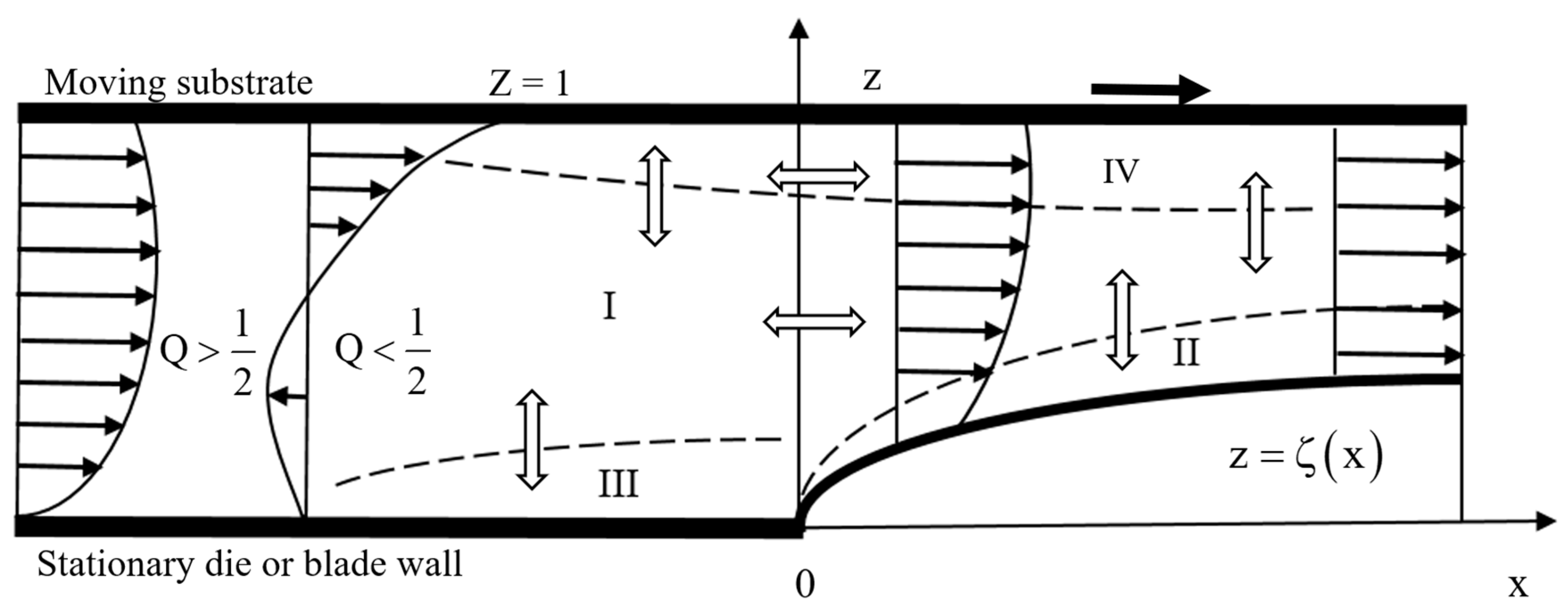
Table 1.
Constants arising in the solution of and .
Table 2.
Influence of flow rate on matching location and corresponding film thickness between the flow near the exit and the flow far from the exit.
Table 2.
Influence of flow rate on matching location and corresponding film thickness between the flow near the exit and the flow far from the exit.
| G | |||
|---|---|---|---|
| 0.0173 | 0.7690 | 0.5 | 0 |
| 0.0206 | 0.825 | 0.6 | −0.6 |
| 0.0442 | 0.824 | 0.7 | −1.2 |
| 0.1539 | 0.814 | 0.8 | −1.8 |
| 0.5824 | 0.865 | 0.9 | −2.4 |
Publisher’s Note: MDPI stays neutral with regard to jurisdictional claims in published maps and institutional affiliations. |
© 2020 by the authors. Licensee MDPI, Basel, Switzerland. This article is an open access article distributed under the terms and conditions of the Creative Commons Attribution (CC BY) license (http://creativecommons.org/licenses/by/4.0/).
Share and Cite
MDPI and ACS Style
Khayat, R.E.; Hossain, M.T. Coating Flow Near Channel Exit. A Theoretical Perspective. Fluids 2020, 5, 180. https://doi.org/10.3390/fluids5040180
AMA Style
Khayat RE, Hossain MT. Coating Flow Near Channel Exit. A Theoretical Perspective. Fluids. 2020; 5(4):180. https://doi.org/10.3390/fluids5040180
Chicago/Turabian StyleKhayat, Roger E., and Mohammad Tanvir Hossain. 2020. "Coating Flow Near Channel Exit. A Theoretical Perspective" Fluids 5, no. 4: 180. https://doi.org/10.3390/fluids5040180