A Relaxation Filtering Approach for Two-Dimensional Rayleigh–Taylor Instability-Induced Flows


School of Mechanical and Aerospace Engineering, Oklahoma State University, Stillwater, OK 74078, USA
*
Author to whom correspondence should be addressed.
Fluids 2019, 4(2), 78; https://doi.org/10.3390/fluids4020078
Submission received: 12 February 2019
/
Revised: 10 April 2019
/
Accepted: 16 April 2019
/
Published: 21 April 2019
(This article belongs to the Special Issue Multiscale Turbulent Transport)
Abstract
:In this paper, we investigate the performance of a relaxation filtering approach for the Euler turbulence using a central seven-point stencil reconstruction scheme. High-resolution numerical experiments are performed for both multi-mode and single-mode inviscid Rayleigh–Taylor instability (RTI) problems in two-dimensional canonical settings. In our numerical assessments, we focus on the computational performance considering both time evolution of the flow field and its spectral resolution up to three decades of inertial range. Our assessments also include an implicit large eddy simulation (ILES) approach that is based on a fifth-order weighted essential non-oscillatory (WENO) with built-in numerical dissipation due to its upwind-based reconstruction architecture. We show that the relaxation filtering approach equipped with a central seven-point stencil, sixth-order accurate discrete filter yields accurate results efficiently, since there is no additional cost associated with the computation of the smoothness indicators and interface Riemann solvers. Our a-posteriori spectral analysis also demonstrates that its resolution capacity is sufficiently high to capture the details of the flow behavior induced by the instability. Furthermore, its resolution capability can be effectively controlled by the filter shape and strength.
1. Introduction
Rayleigh–Taylor instability (RTI) is an interfacial hydrodynamic instability that occurs at the interface separating two fluids of different densities in the presence of relative acceleration [1]. Understanding the behavior of the RTI-induced flows are of great importance because of the prevalence of such instability phenomena in many natural, industrial, and astrophysical systems with unstably stratified interfaces, such as coastal upwelling near the surface of the oceans [2], atmosphere and clouds [3], plasma physics such as magnetic or inertial confinement fusion implosions [4], the ignition of supernova [5,6], air bubble formation in the blood of deep sea divers [7], premixed combustion [8,9] and many more. In general, RTI phenomenon is one of the easiest hydrodynamics instabilities to observe, for example, if we invert a glass filled with water, the RTI occurs which makes the water falling [10,11]. Lord Rayleigh first described theoretically an instability that occurs in Cirrus cloud formation when a dense fluid is supported by a lighter one in a gravitational field [12]. Later Sir G. Taylor demonstrated the same instability experimentally for accelerated fluids [1], and honouring to their contributions, this instability is named after Lord Rayleigh and Sir G. Taylor which is the Rayleigh–Taylor instability. A detailed overview of the application of RTI phenomena with definitions, physical interpretations and terminologies can be found in [13,14,15,16,17]. Although RTI is a part of many diverse areas of scientific research, and there have been a substantial body of works conducted on this instability over the last few decades, still there have been many open questions yet to be answered about the nature of the RTI-induced flows [18,19,20]. Moreover, the numerical simulation of RTI studies was not popular much before the 1980s due to the limitation of computational resources. Additionally, the simulation of the flows with RTI is comparatively challenging task since the instability grows up from small scales to initiate secondary instabilities. With a goal to enhance our understandings of RTI phenomenon numerically, the main purpose of this paper is to resolve and analyze the flow field of the RTI test problem with two different initial condition setups using the relaxing filtering modeling approach and compare the high- and coarse-resolution simulation results with the traditional ILES-Riemann solver simulation results.
With the advancement of computational resources, numerical study of RTI has become popular to many research groups for last few years. However, many of the earlier numerical studies in this direction show some variations in the results, such as growth rates of mixing or instability, from the experimental results [21] and it was required to find more improvements in model development and in finding the parameter dependence on the problem setup. Nevertheless, for the last few years, there have been a considerable number works conducted on developing our understandings on RTI related problems [20,22,23,24,25,26,27,28,29,30,31,32]. In general, the single-mode RTI is studied most and has also been used as a building block for multi-mode RTI development [20]. Among some recent notable works on RTI study, the late-time growth in single-mode RTI was studied in [20,31]. In [31], the authors used the implicit large eddy simulation (ILES) approach in a three-dimensional computation of RTI whereas in [20], the author illustrated the growth stages in single-mode RTI using direct numerical simulation (DNS) for two-dimensional computational domain. The formation of the Kelvin-Helmholtz (KH) roll-up of the spike for two-dimensional single-mode RTI simulation was shown in [33]. In [25], it was found that the two-dimensional flow simulation results vary substantially from the three-dimensional ones. Also, it was observed in other literature that the two-dimensional single-mode RTI flows grow faster than the three-dimensional ones [26,34,35]. Youngs et al. [36,37,38] also studied on the comparison between two and three-dimensional RTI to find out the variation in growth rate at different time stage of the simulations. Also, the authors showed the level of mixing was lower for two-dimensional case. For the multi-mode RTI simulations, similar findings have been shown for growth rate of mixing layer of both two and three-dimensional test setup in [36,39,40]. On the other hand, Zhou et al. and Shvarts et al. [41,42] did a scaling analysis of RT turbulence. In his seminal paper, Chertkov [43] proposed a phenomenological theory for the two-dimensional RT system corresponding to so-called Bolgiano scaling. Quantitatively, also explained in [16], the theory leads to the scaling for velocity spectrum, and scaling for the density/temperature spectrum. Such theoretical predictions have been also confirmed by direct numerical simulations [44]. In this investigation, we consider the two-dimensional computational domain since it is computationally economical, and we can investigate such scaling behaviors in simulating flows with large inertial range. In our two-dimensional setup, we simulate both multi-mode and single-mode RTI cases using relaxation filtering and ILES modeling approach and obtain the density field contour and kinetic energy spectra to analyze the two-dimensional flow behavior. Our primary focus of this work is to compare between the numerical models implemented on this particular test problem through analyzing the density field plots and statistical tools. However, we will also analyze the resolution and scale resolving capacity of both models through high-resolution simulations.
Numerical simulation of the turbulent flows with instabilities has always been a challenging task since the turbulent features and discontinuities coexist in the flow for a very large spatial and temporal scales. Resolving these enormous scales not only require a huge amount of computational resources but also development of a suitable scheme which has the regularization capability to prevent any oscillations near the discontinuities or shocks. A desired scheme should add a sufficient amount of artificial numerical dissipation near the instability to capture the shocks; however, it should not be too dissipative to damp the small-scale structures of the flow. Over the years, a vast number of successful shock-capturing algorithms have been introduced. For any numerical examination or assessment of a turbulent flow governed by Eulerian hyperbolic conservation laws, ILES methodology can be a good choice to consider which is proven to show a good performance on resolving turbulent flows with shock and discontinuities [45,46,47,48]. One of the popular ILES framework is to use an upwind scheme (e.g., Weighted Essentially Non-Oscillatory (WENO) scheme) along with a Riemann solver to incorporate the artificial through the use of numerical truncation errors [49]. The upwind-biased and nonlinearly weighted WENO schemes are widely used in resolving highly compressible turbulent flows because of their robustness to capture discontinuities in shock dominated flows and high order of accuracy in preserving turbulence features [50,51,52]. It should be mentioned that the development of improved WENO scheme is an active research field and still, there are a lot of works going on in this research direction [53,54,55,56]. Another candidate modeling approach is the explicit filtering approach using relaxation filtering which add dissipation on the truncated scales in LES through a low-pass filter [57,58,59,60]. In this approach, an additional low-pass spatial filter is used to estimate the effect of unresolved scales. The selection of relaxation filter also affects the solution field for explicit filtering approach and there are a significant number of literature available on the formulation of suitable and efficient LES filters [61,62,63]. In this work, we use the sixth-order symmetric central scheme with a 7-point stencil Simpson’s filter (SF7) as a relaxation filter for RTI test case. We also implement ILES scheme combined with Roe and Rusanov Riemann solver to compare the results obtained by our relaxation filtering solver. The main purposes of this paper are to simulate RTI-induced flow (for both single and multi-mode perturbation) using a relaxation filtering approach to observe the resolution capability of this scheme, analyze the flow behavior by observing the density field contours, and compare the results obtained by relaxation filtering scheme and ILES scheme through kinetic energy (with and without density-weighted velocity) and power density spectra plots. The results show that the relaxation filtering scheme captures more scale in inertial subregion whereas the ILES scheme resolves more scales in high wavenumber regime. For both multi-and single-mode RTI, the kinetic energy spectra plots tend to follow the scaling law. On the other hand, the power density spectra plots are observed to be aligned to at high resolution. More rigorous derivations and mathematical analyses of scaling laws can be found elsewhere [64,65,66,67,68,69]. Also, the density contour plots for single-mode RTI reveal that the symmetry of the falling spike break at high resolution because of the formation of secondary instabilities from smaller scales resolved at high resolution. However, the lower resolution simulations resolve the symmetry for all schemes since the numerical dissipation surpasses the formation of the secondary instabilities. Also, it has been seen that the filter strength of the relaxation filter allows us to add more or less dissipation to the solver which eventually affects the flow behavior.
The rest of the paper is organized as follows. Section 2 gives a brief description of the governing equations. Section 3 illustrates the numerical methodology implemented in this study. In Section 4, we detail the results obtained by the numerical schemes used in our investigation along with the problem definitions of the RTI test problem. We demonstrate our findings through high- and coarse-resolution density field contour and density-weighted energy spectra plots. Section 5 gives the summary of our findings and conclusions.
2. Governing Equations
In our study, we consider two-dimensional Euler equations in their conservative dimensionless form as underlying governing equation for the Rayleigh–Taylor instability-induced flow evolution and can be expressed as:
where F, G account for the inviscid flux contributions to the governing equation and S represents the gravitational term acting on the vertically downward direction (i.e., ). The quantities included in q, F, G and S are:
Here, , p, e, u, and v are the density, pressure, total energy per unit mass, and the horizontal and vertical velocity components, respectively. The total enthalpy, h and pressure, p can be obtained by:
where is chosen as the ratio of specific heats in our study. We refer the reader to [50,70] for details on the development of the eigensystem of the equations to devise hyperbolic conservation laws.
3. Numerical Methods
To develop the computational algorithm for our test problem governed by hyperbolic conservation laws, we formulate a finite volume framework by using different numerical strategies and schemes. In this section, we briefly introduce the numerical methods considered in the present study. We use the method of lines to cast our system of partial differential equations given in Equation (1) in the following form of ordinary differential equation through time:
where is the cell-averaged vector of dependent variables, and represents the convective flux terms in the governing equation which can be expressed in the following discretized form:
Here, are the cell face flux reconstructions in x-direction and are the cell face flux reconstructions in y-direction. We use the optimal third-order accurate total variation diminishing Runge-Kutta (TVDRK3) scheme [71] for the time integration:
where the time step, should be obtained by (satisfying the Courant-Friedrichs-Lewy (CFL) criterion):
where a is the speed of the sound that can be computed from the primitive flow variables (i.e., ). In our current investigation, we use for all the simulations ( for numerical stability). For the cell face flux reconstructions, we have implemented the ILES and relaxation filtering modeling approaches on our test problem which will be discussed briefly in the subsequent sections.
3.1. ILES Approach
To develop our ILES framework, we first use the WENO interpolation scheme to reconstruct the left and right state of the cell boundaries. Later, we calculate the fluxes at cell edges from the reconstructed left and right states using a Riemann solver. The finite volume framework of a system of Euler conservation equations usually requires a Riemann solver to avoid the Riemann problem [72]. The damping characteristics of nonlinear WENO schemes acts as an implicit filter to prevent the energy accumulation near the grid cut-off [73,74]. In this work, we use the 5th order accurate WENO scheme followed by two widely used Riemann solver, Roe and Rusanov Riemann solver, to determine the flux at cell boundaries.
3.1.1. Weno Reconstruction
The WENO scheme is first introduced in [75] for problems with shocks and discontinuity to get an improvement over the essentially non-oscillatory (ENO) method [76,77]. In this work, we use an implementation of the WENO reconstruction using 7-point stencils (i.e., updating any quantity located at index i depends on the information coming from , , ..., ) which can be written as:
Here, and are the left state (positive) and right state (negative) fluxes, respectively, approximated at midpoints between cell nodes. The left (L) and right (R) states correspond to the possibility of advection from both directions. Since the procedures are similar in the y-direction, we shall present stencil expressions only in the x-direction for the rest of this document. are the nonlinear WENO weights of the stencil where and r is the number of stencils ( for the WENO5 scheme). The nonlinear weights are proposed by Jiang and Shu [78] in their classical WENO-JS scheme as:
but the nonlinear weights defined by the WENO-JS scheme are found to be more dissipative than many low-dissipation linear schemes in both smooth region and regions around discontinuities or shock waves [79]. In our study, we have used an improved version of WENO approach proposed by [80], often referred to as WENO-Z scheme. One of the main reasons behind selecting WENO-Z can be less dissipative behavior than classical WENO-JS to capture shock waves. Also, there is a smaller loss in accuracy at critical points for improved nonlinear weights. The new nonlinear weights for the WENO-Z scheme are defined by:
where and p are the smoothness indicator of the stencil and a positive integer, respectively. Here, , a small constant preventing zero division, and is set in the present study to get the optimal fifth-order accuracy at critical points. The expressions for in terms of cell values of q are given by:
are the optimal weights for the linear high-order scheme which are given by:
3.1.2. Roe Riemann Solver
Based on the Godunov theorem [72], Roe developed an approximate Riemann solver, known as the Roe Riemann solver [81]. In our computational algorithm, we use the flux difference splitting (FDS) scheme of Roe [81] where the exact values of the fluxes at the interface can be computed in the x-direction by:
Here, is the flux difference, calculated as:
where
Here, denotes the difference between right and left state fluxes for the variables (e.g., ), and eigenvalues are defined as , and , where is the speed of the sound at averaged state. In the equations, the tilde represents the density-weighted average, or the Roe average, between the left and right states. The Roe average values can be found by:
where the left and right states of the un-averaged conserved variables are available from the WENO5 reconstruction described earlier. However, it is later realized that the stationary expansion shocks are not dissipated appropriately by this method. To fix the entropy in the expansion shocks, Harten proposed the following approach [82] replacing Roe averaged eigenvalues by:
Here, where is a small positive number, is set in our computations. Similarly, in y-direction, , and . The interfacial fluxes in y-direction can be estimated by:
where
with
where , , , and .
3.1.3. Rusanov Riemann Solver
Rusanov proposes a Riemann solver based on the information obtained from maximum local wave propagation speed [83], sometimes referred to as local Lax-Friedrichs flux [84,85]. The expression for Rusanov solver in the x-direction is as follows:
where the right constructed state flux component, is , the left constructed state flux component, is and the characteristic speed, . The density-weighted average of the conserved variables can be calculated by Equation (18). Similarly, the expression for Rusanov solver in y-direction is:
where .
3.2. Central Scheme with Relaxation Filtering (Cs+Rf) Approach
In our relaxation filtering approach, we consider a symmetric flux reconstruction using a purely central scheme (CS) combined with a low-pass spatial filter, 7-point stencil Simpson’s filter (SF7) in our case, as a relaxation filter (RF). We denoted this solver as CS+RF. For the cell interfacial reconstruction of the conserved quantity, the following symmetric non-dissipative scheme is used [86]:
for the interpolation in x-direction, and similarly in y-direction, the conservative interpolation formula reads:
where the stencil coefficients are given by:
Here, represents the flow variables (at cell centers) given in Equation (4). The calculated fluxes from the relevant face quantities determined from the nodal values can be used in discretized finite volume equation. In this approach, we assume that the explicit filtering removes the frequencies higher than a selected cut-off threshold through the use of the low-pass spatial filter. A low-pass filter is commonly used in explicit filtering approaches which can be considered to be a free modeling parameter with a specific order of accuracy and a fixed filtering strength [87]. The filtering operation is done at the end of every timestep to remove high frequency content from the solution which eventually prevents the oscillations [58,88,89]. A discussion and analysis of the characteristics on different low-pass filter can be found in [90]. In our investigation, the expression for the sixth-order sequential RF for any quantity f is:
where
Here, the discrete quantity yields the filtered value and the filtering coefficients are:
and is a parameter that controls filter dissipation strength in a range of where indicates no filtering effect at all, i.e., completely non-dissipative and indicates the highest filtering effect, i.e., most dissipative with a complete attenuation at the grid cut-off wavenumber. The transfer function of the SF7 filter displays a trend of more dissipation with the increase of the parameter [49].
4. Results
In this section, we present our numerical assessment of the modeling approaches outlined in the previous section for both multi-mode and single-mode two-dimensional RTI test problem. We first illustrate the problem definitions of our test case which is followed by the results obtained by different numerical solvers. We perform our quantitative comparisons between the ILES and CS+RF models using the density contours, density-weighted kinetic energy spectra, and compensated density-weighted kinetic energy spectra plots. For comparative analysis, we obtain the high-resolution ILES and CS+RF solutions by using a parallel computing approach using the Open Message Passing Interface (MPI) framework [91,92]. A detailed discussion on the MPI methodology implemented in our study can be found in [49]. Using both high- and coarse-resolution simulation results, the scaling behaviors of the kinetic energy spectra plots are also investigated in this section.
4.1. Two-Dimensional RTI Test Problem: Case Setup
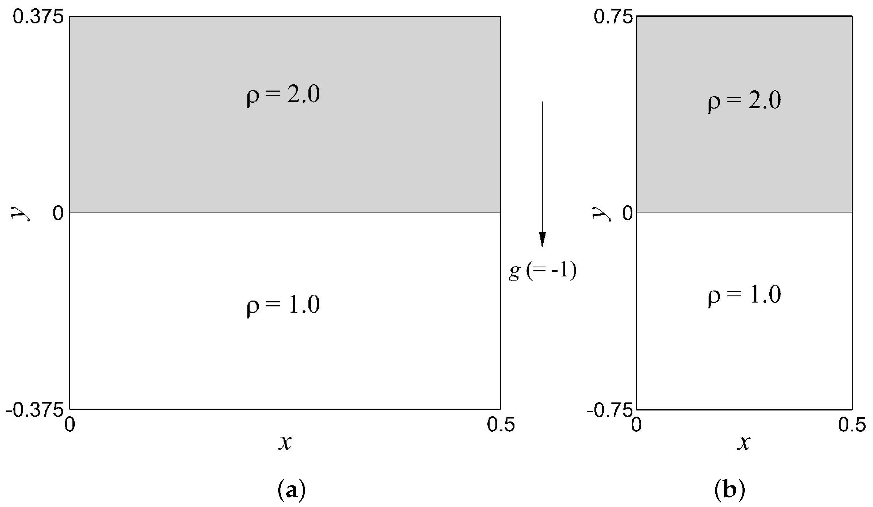
In our numerical experiments, we use a two-dimensional implementation of RTI using the aforementioned numerical schemes. In general, RTI arises at the interface of two fluids when a dense fluid is supported above a comparatively lower density fluid in a gravitational field or stay in the presence of relative acceleration. Since it is found in numerous literature that many properties related to the RTI-induced flows such as the overall growth rate of RTI mixing, dissipation scales, velocity field, and so on, more or less depend on the initial conditions of the flow domain [14,93,94,95], we consider RTI with multi-mode or randomized perturbation and RTI with single-mode perturbation in our study. We first focus on the case of randomized initial perturbation where our computational domain is set with the following initial conditions:
Here, is set and the amplitude of the perturbation is set at and is a random number with a value in between 0 and 1. Since is updating itself at each grid point, we note that it is an implicit function of both x and y. On the other hand, for the single-mode RTI, the computational domain is set with the following initial conditions:
where and is set and respectively with the similar amplitude of the perturbation as the multi-mode case, . The similar two-dimensional RTI test problem set up has been used in various studies related to RTI [96,97]. Figure 1 shows the schematic of the computational domain for both cases of the RTI test problem where it can be seen that we consider the normalized gravity is acting in vertically downward direction in our problem definitions.
We must note here that we apply the periodic boundary condition on the left and right boundaries, and the reflective boundary condition on the top and bottom boundaries of our computational domain for both test setup. To get a better understanding on the boundary conditions used in our test setup domain, we can consider an arbitrary two-dimensional domain illustrated in Figure 2. To apply the periodic and reflective boundary condition for our 7-point stencil scheme, we take three ghost points in each direction of the four boundaries of our computational domain. For periodic boundary condition on the left and right boundaries, the ghost point values of the time-dependent variables in vector q (from Equation (2)) can be computed by:
where . On the other hand, our approximation for the reflective boundary condition is as follows:
where . For the parallelization, we do the domain decomposition in the y-direction and update the ghost points of the local domain by transferring the information from the adjacent domain. Although we implement our reflective boundary conditions as defined by Equation (39), we note that the boundary conditions are often applied on the velocity rather than momentum. We stress that simulations of unsteady compressible flows require an accurate control of wave reflections from the boundaries of the computational domain since such waves may propagate from the boundary and interact with the flow [98]. We plan to implement more accurate characteristics-based boundary conditions in our future studies.
4.2. RTI with Random (Multi-Mode) Perturbation
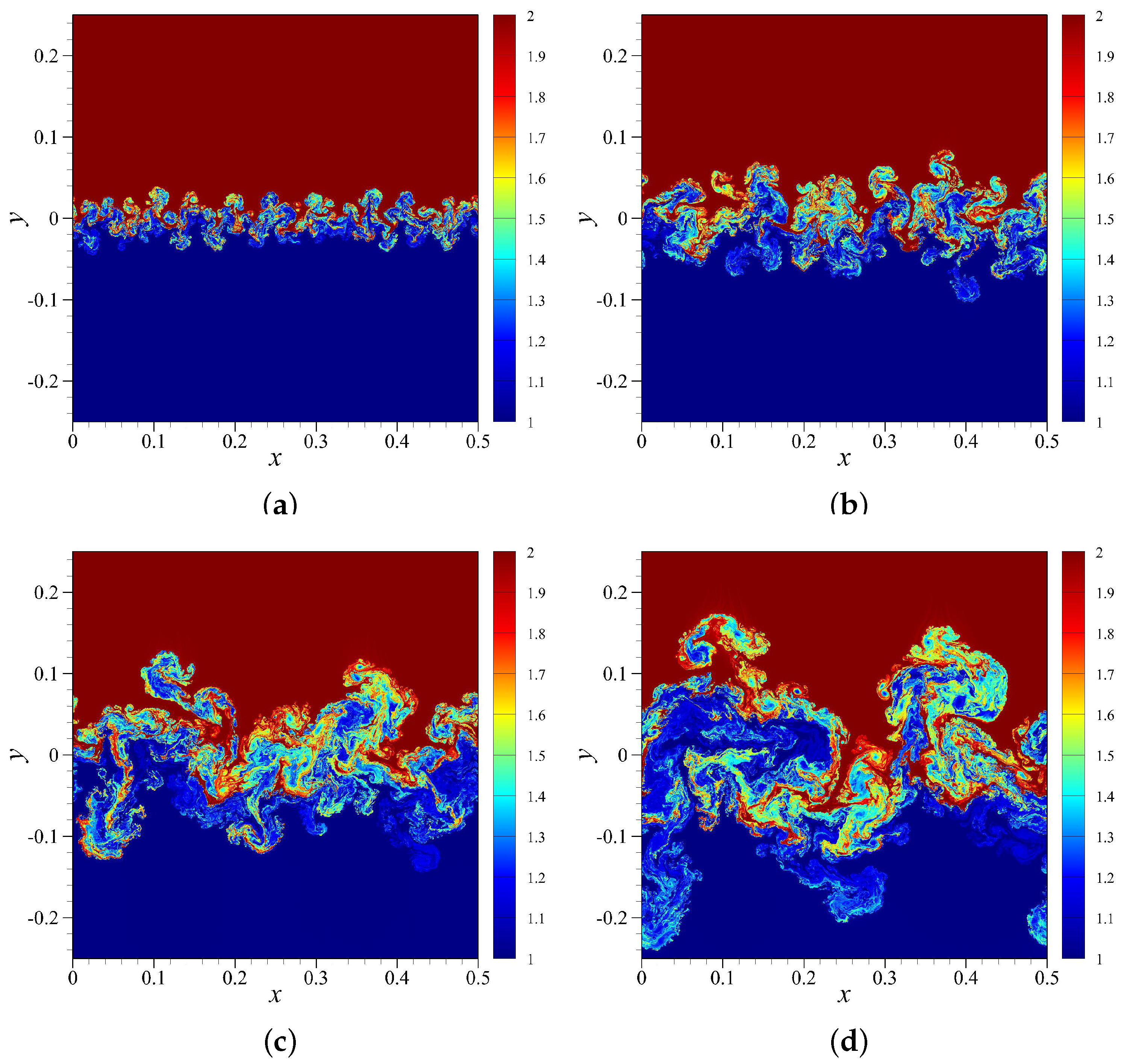
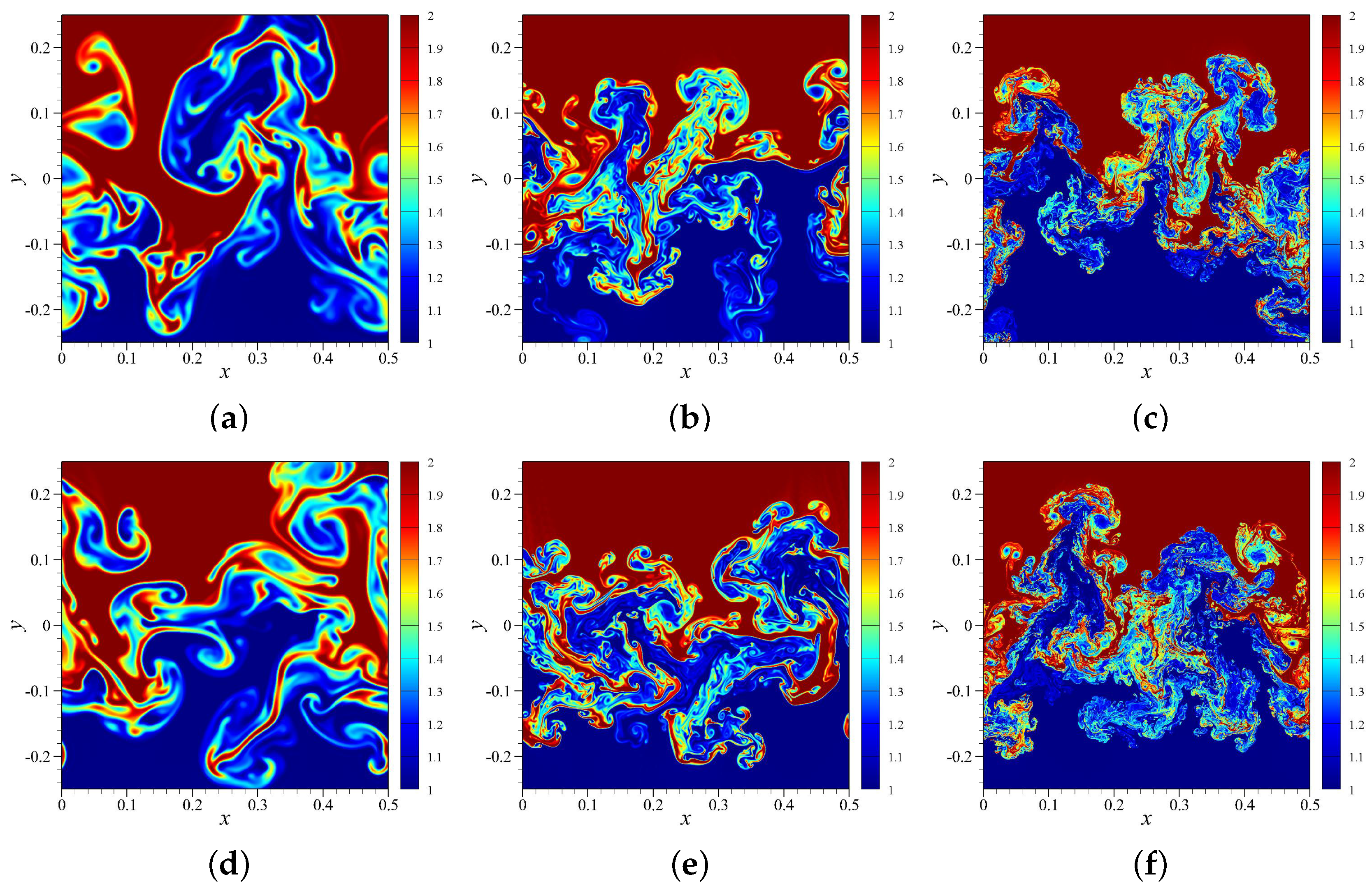
The nonlinear evolution of the Rayleigh–Taylor instability from multi-mode initial perturbations is studied based on the density field contour and density-weighted kinetic energy spectra to assess the performance of the underlying modeling schemes. Figure 3 shows the time evolution of the density field at high resolution using the ILES-Roe scheme. As it is shown in [99] that the DNS and ILES give similar results for global properties of RTI-induced mixing, we use the high-resolution results of ILES schemes to avoid the higher computational cost of DNS. Also, it is apparent in Figure 3 that several fine scale structures are captured using the ILES-Roe scheme because of its capability to resolve the smaller scales in high wavenumber region. It can be observed that the mixing growth rate is uniform along the interface at with multiple modes. It has been seen before in [21] where authors found a uniform growth of the mixing region initially for an idealized initial condition whereas the experimental results of same test condition show the presence of dominant scale at the same time. In our study, even though there are some dominant scales or modes present at , there are a considerable amount of unmixed region can be seen at the same time which indicates the slow mixing rate for this initial condition. In Figure 4), we present the density contour plots for coarse-resolutions obtained by different ILES-Riemann solver combinations at final time of our simulation, i.e., at . As we can see, a clear difference in the growth of scales as well as mixing for both solvers. Since the Rusanov solver is more dissipative than the Roe solver [100], it is expected to have different evolution of the scales in the flow field. Similarly, we can observe different flow field evolution of CS+RF scheme for different filtering strength, in Figure 5. Since the higher value of adds more dissipation, this solver induces different amount of perturbation in the flow field with the evolution of time than the solver with lower value of . Hence, we plot the density-weighted kinetic energy spectra to get a better view in the performance of different solvers [27,101,102,103,104]. To include these density effects, we define the energy spectrum built on density-weighted velocity vector which can be expressed as:
where the density-weighted velocity components are
We then can calculate the density-weighted kinetic spectra by following expressions:
where k refers to the wavenumber along x-direction. We obtain the Fourier coefficients using a standard FFT algorithm [105]
where i refers to unit imaginary number, and (, ) determines the Cartesian grid. Since our domain is periodic only in x-direction, we note that our spectra calculations are averaged in y-direction as illustrated in Equation (43). The other statistical measures investigated in our study are the classical kinetic energy spectra and power density spectra. The energy spectra can be calculated using the following definition in wavenumber space [106]:
where the velocity components and can be computed using a similar fast Fourier transform algorithm presented in Equation (44). To quantify the effect of the scale content of density field, we use the power spectrum that reflects the average packaging of density over different scales at any given time in the simulation. This may be given by the following expression:
where is the Fourier coefficients of the density field.
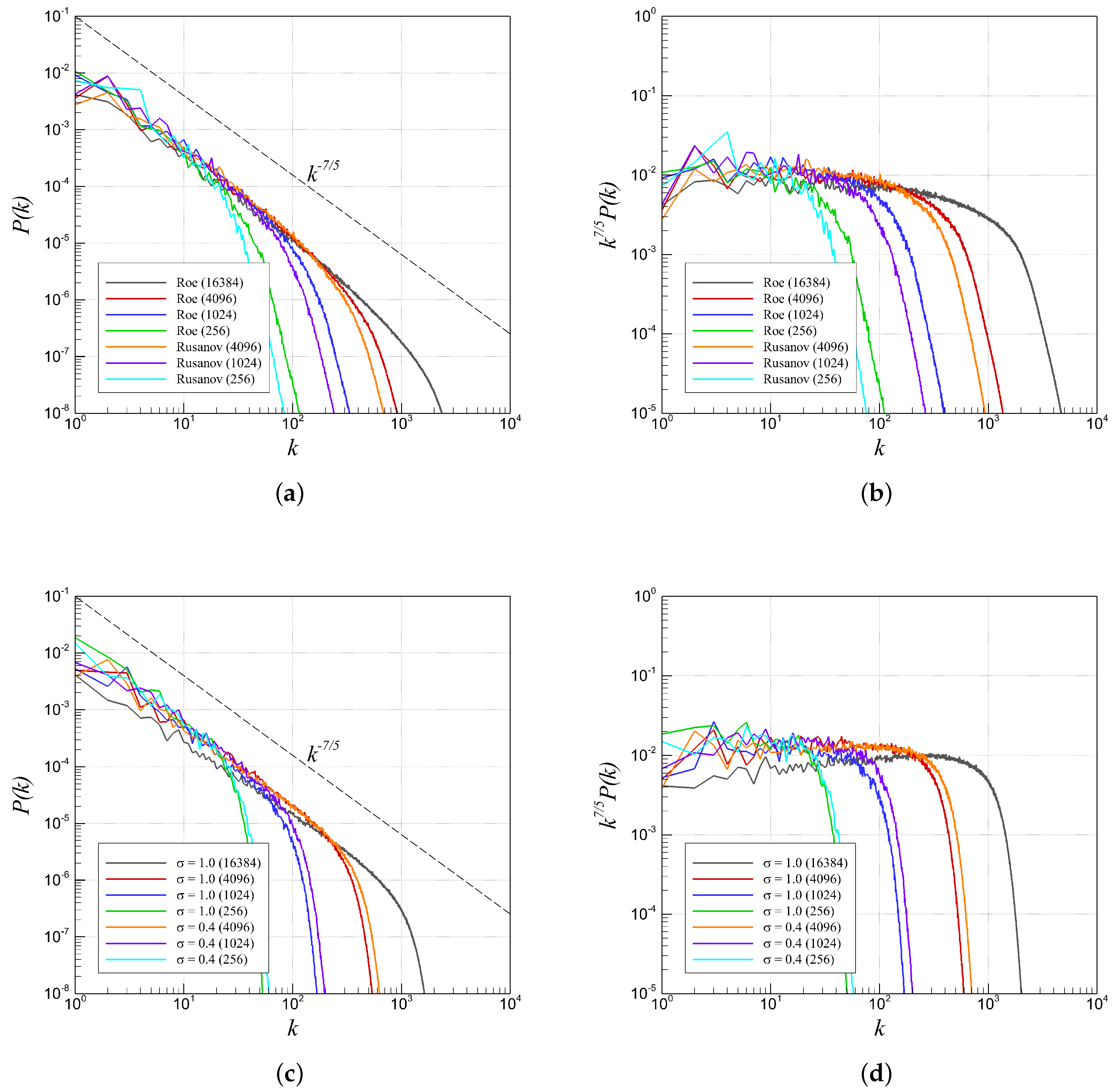
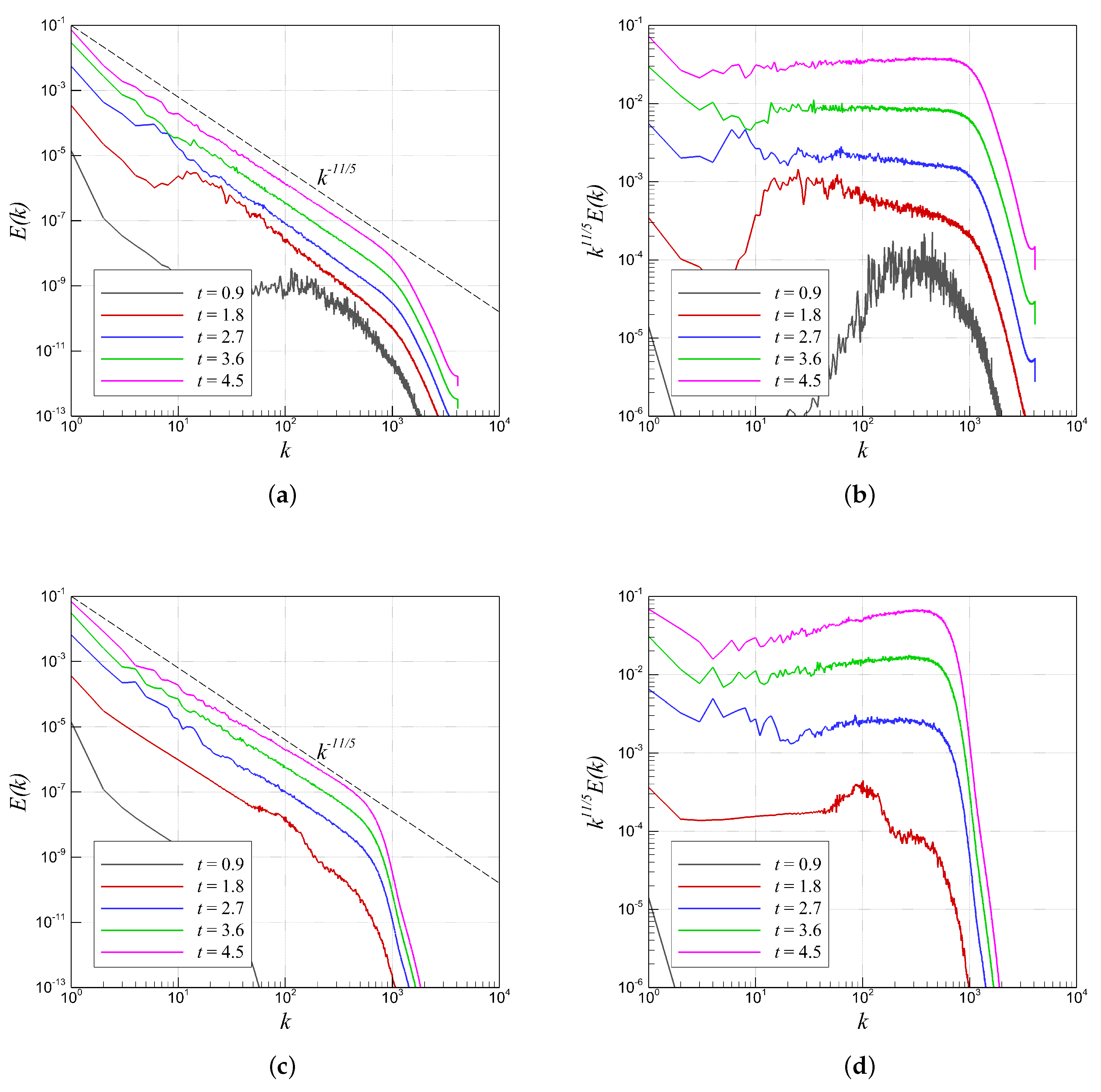
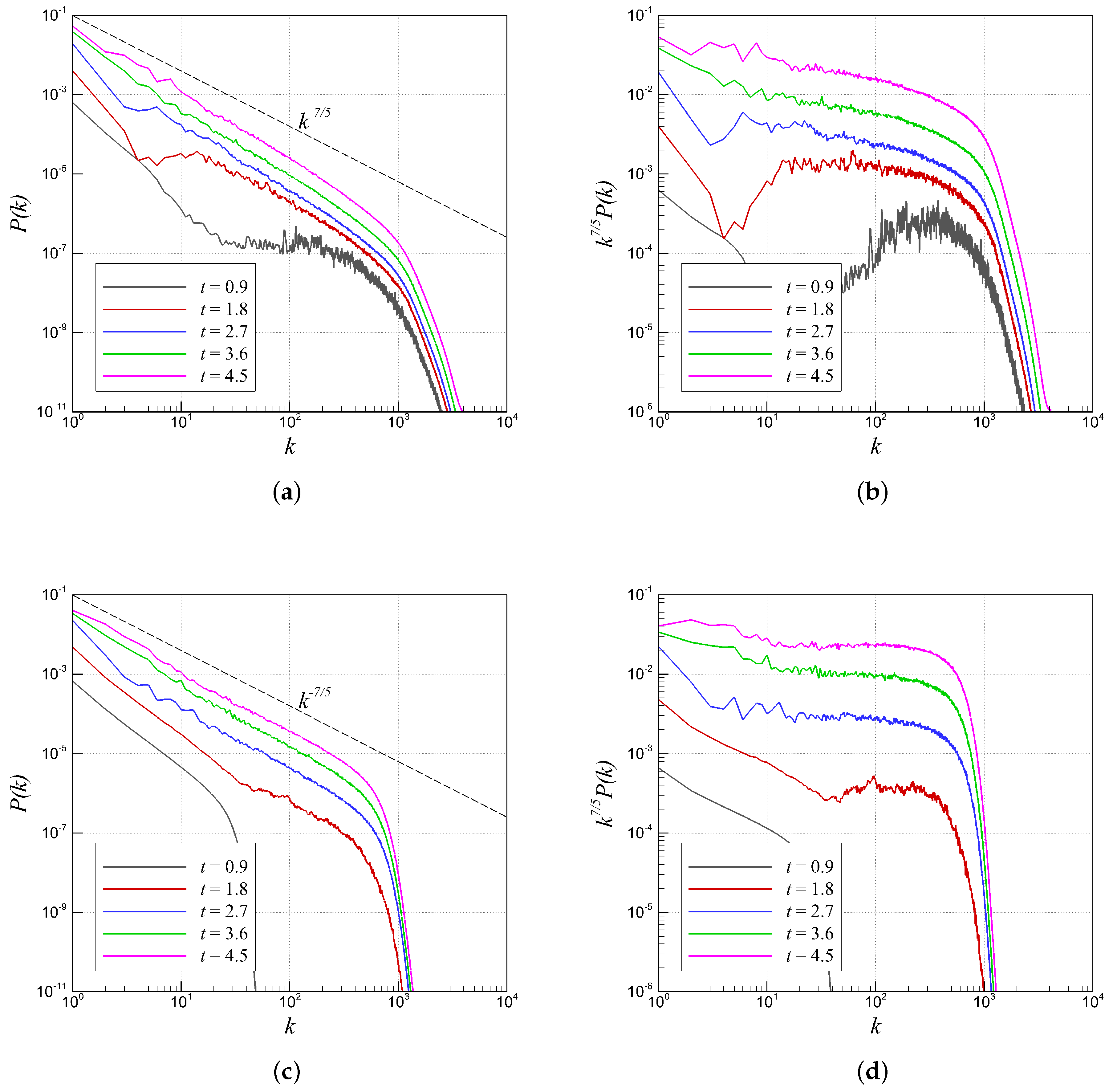
For the validation of our spectra plots, we follow the well-established theory for two-dimensional RTI systems [14,43,44]. In his seminal paper, Chertkov [43] proposed a phenomenological theory corresponding to the Bolgiano scaling [107] which can be abstracted to scaling law for density or temperature and scaling law for velocity. In Figure 6, we can see that the spectra plots (on the left) obtained by the ILES and CS+RF schemes are showing a clear inertial subrange with the scaling. However, it is apparent that the CS+RF scheme results are the most aligned with the reference line. Moreover, we present the kinetic energy spectra plots without density weighting in Figure 7 which supports the conclusions of the density-weighted energy spectra plots. To validate further, we plot the regular and compensated power density spectra in Figure 8 where it can be seen that the density spectra for CS+RF scheme are following the scaling law.
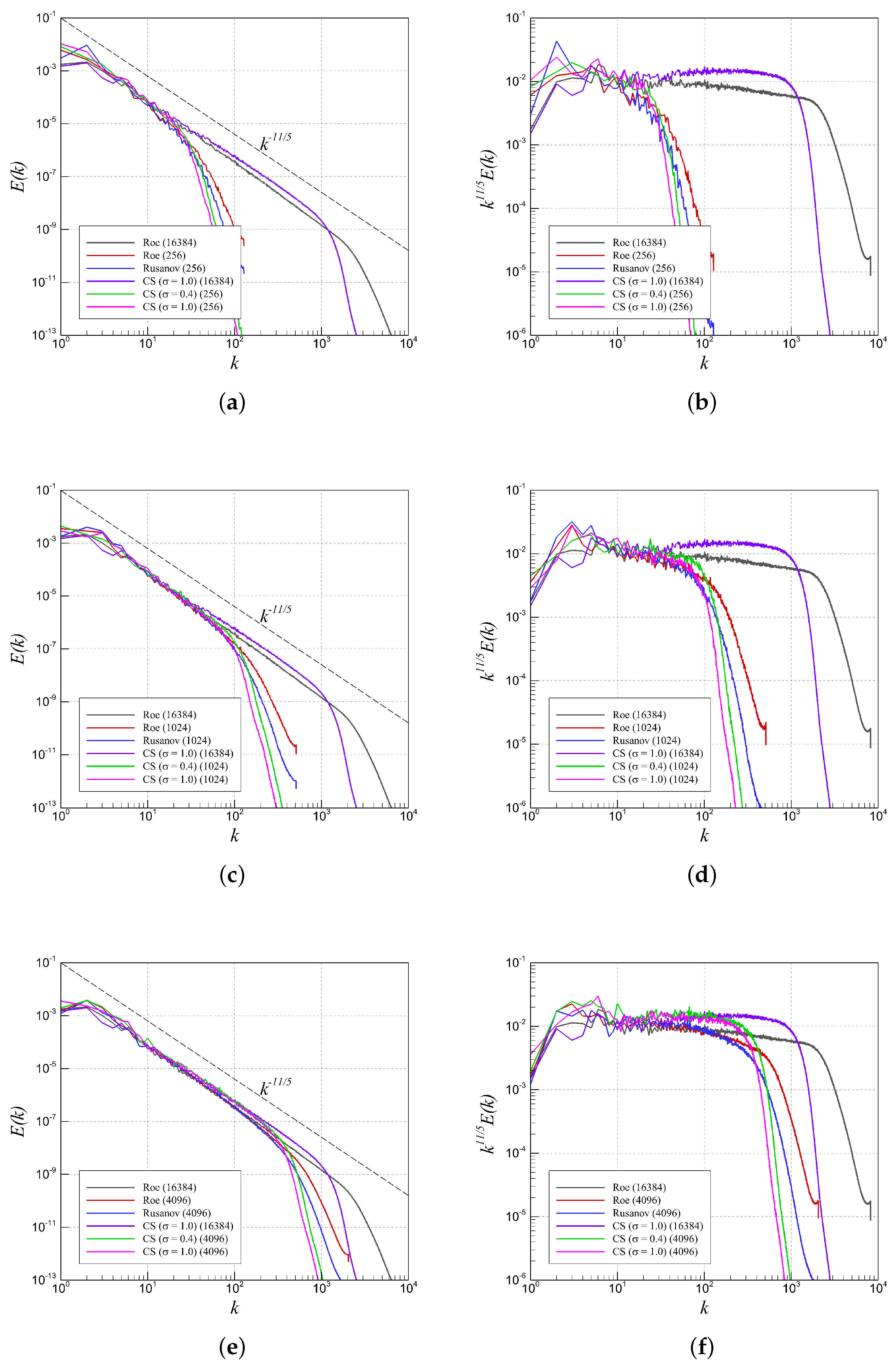
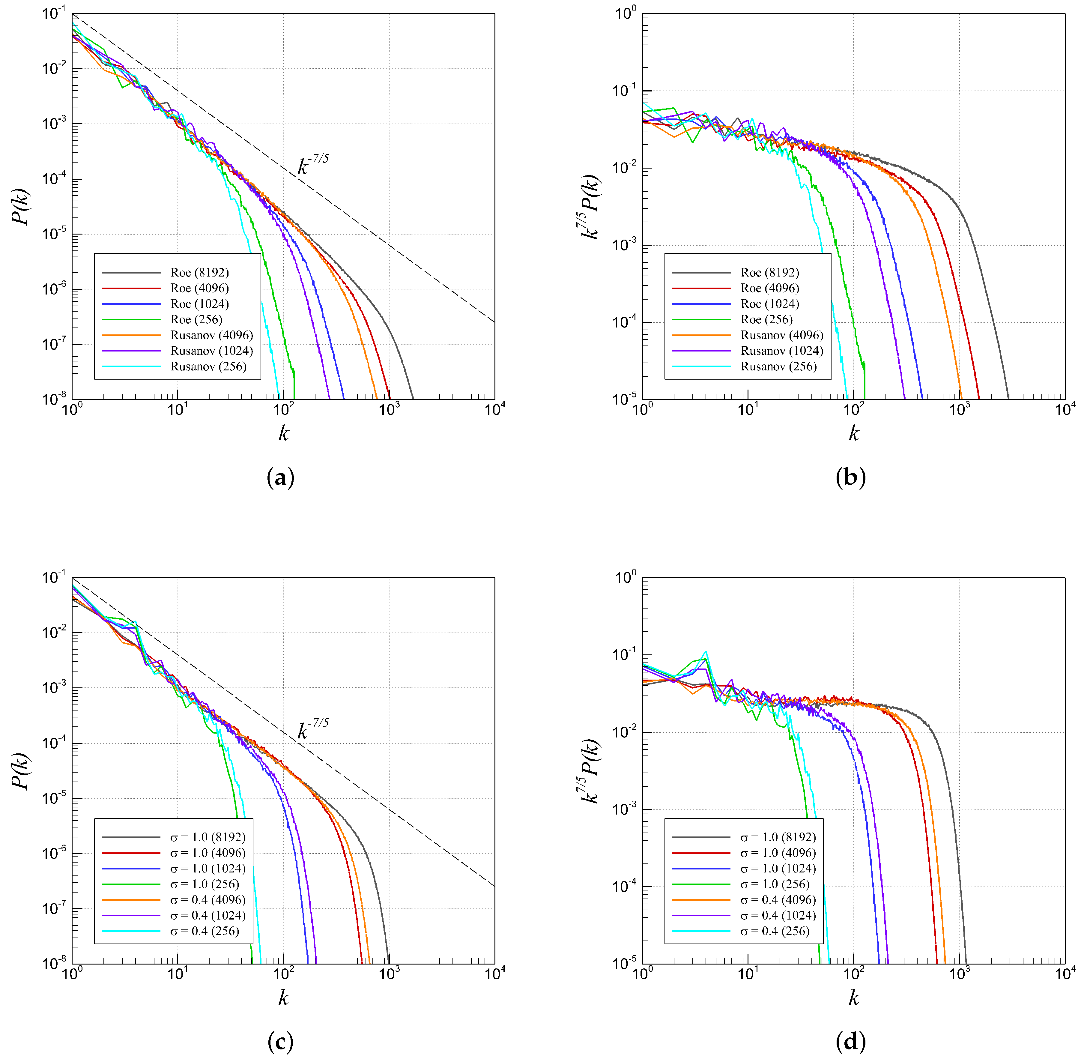
The time evolution of the spectra shows similar statistical trends for all schemes. Therefore, we will only focus on the results at final time in our subsequent analyses. To compare the dissipation characteristics of the schemes, we place the density-weighted spectra of both ILES schemes in a single plot as well as for both CS+RF scheme with different filtering strength in Figure 9. It can be observed that the Rusanov solver is more dissipative than the Roe solver and the higher value adds more dissipation. These findings are consistent with the previously found results in the literature as well. Also, the spectra are following the reference scaling. The density-weighted spectra plots compensated by for the CS+RF scheme with different filtering strength show that all the lines are flat above the axis line. However, the kinetic energy spectra plots without the density weighting in Figure 10 exhibit a similar trend as the density-weighted ones. On the other hand, the power density spectra plots in Figure 11 show that the scaling law is maintained for both set of schemes. However, the compensated spectra plots indicate that the CS+RF scheme is more consistent with the scaling law than the ILES schemes. We present another set of density-weighted spectra plot varying grid resolution to show a comparison between the ILES and CS+RF schemes in Figure 12. It is apparent that the CS+RF captures more scales in the inertial subrange than the ILES schemes. However, the CS+RF scheme reaches the effective grid cut-off scales earlier than the ILES schemes. It is because the CS+RF solvers do the filtering once at the end of the simulation whereas the ILES solvers implicitly adds dissipation throughout the simulation. As a result, ILES schemes capture wide range of scale at high wavenumber even though they resolve comparatively less scales in the inertial subrange. Some key points can be seen from Figure 12 that the solver is the most dissipative among all solvers considered in this study, and solver captures more scales in the inertial subrange than the other solvers. Also, ILES-Roe solver resolves the highest range of scales in high wavenumber for both coarse and high resolution which explains the appearance of very fine small-scale structures in the density field contour plot obtained by ILES-Roe solver.
4.3. RTI with Single-Mode Perturbation
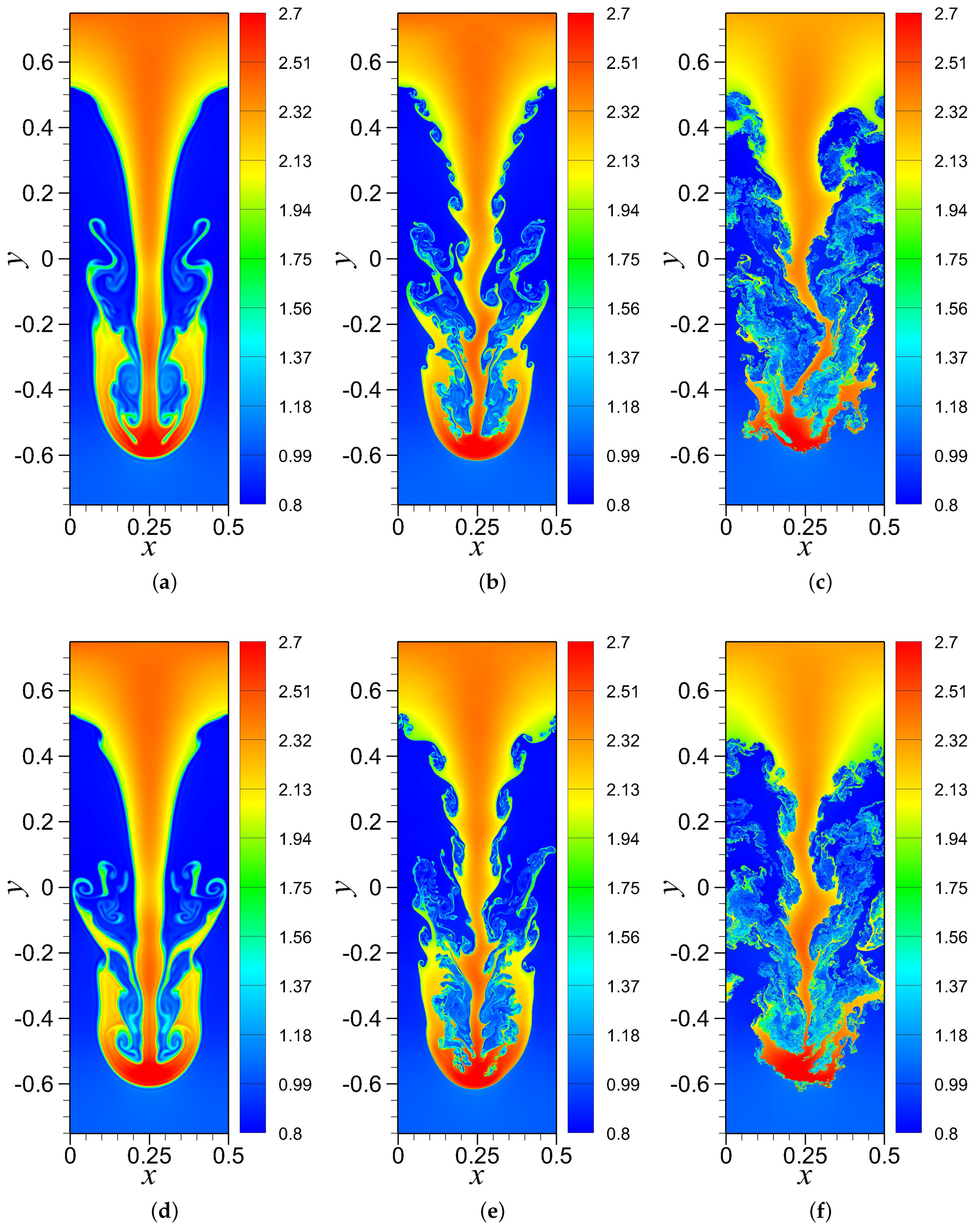
Numerical simulation of flows with RTI is comparatively challenging because the instability grows from the small scales of the flow field [19,108]. Since the analytical modeling can be done for single-mode RTI, the numerical study of the RTI with the single-mode perturbation setup has been started very early [33,109] and still being studied extensively to understand and explain the nature of RTI-induced flows [20,31,32,110,111,112,113]. For our analyses of the single-mode perturbation case, we first present the time evolution of the density field results obtained by ILES-Roe solver at a high resolution of in Figure 13. It is observed in many studies that the tips of the spikes of a single-mode RTI-induced flow always maintains the symmetry [14]. Yet in our simulation, the line of symmetry within the spike of the single-mode RTI in Figure 13 is seen broken at time . This phenomenon was observed and well explained by Ramaprabhu et al. [31] at late-time of the RTI flow simulation which the authors referred to as “chaotic mixing” at the late-time regime. With simulations of the Euler equations, it can be also seen in [96] that the less dissipative schemes show this interface breaking up, while the more dissipative schemes suppress the instability. In our high-resolution simulation, the presence of small-scale structures can be seen in very early stage which lead to secondary instability, i.e., the KH vortex formation as well as chaotic mixing. However, for small or modest grid resolutions, the numerical viscosity suppresses the small-scale structures and preserves the symmetry which can be seen in Figure 14, Figure 15, Figure 16 and Figure 17. In Figure 14, we present the state of the density field at (top row) and (bottom row) for the simulations by using the ILES-Rusanov solver at different grid resolutions. It is apparent that the and resolution results hold the symmetry. But the result shows the development of smaller scales at which leads to the loss of symmetry at final time, . Similar conclusions can be made for the ILES-Roe solver results in Figure 15. However, the loss of symmetry can be observed even in resolution simulation for the ILES-Roe scheme since the ILES-Roe solver is less dissipative compared to the ILES-Rusanov solver. For both CS+RF schemes in Figure 16 and Figure 17, the symmetry holds for lower resolutions and breaks for higher resolution. Since there is no physical viscosity in Euler simulations, we note that the breakup of the interface and the loss of symmetry can be due to the numerics. When increasing the resolution, the loss of symmetry in RTI problems have been also demonstrated in the literature (e.g., see [55,114,115]). Similar observations can be seen when we use the higher-order numerical schemes. We also refer to [116,117] for an illustration of symmetry breaking and increasing mixing in Richtmyer–Meshkov instability problems for solving Euler equations.
Figure 18 presents the density field plots at the final time, , to get a comparative idea between the performance of the ILES schemes. We can observe in Figure 18 that the symmetry is maintained in lower resolutions, but starts to break with the increase of the resolution for both ILES solvers. If we look at the resolution results for both ILES solvers, we can see that the ILES-Roe scheme result is more deviated from the symmetry than the ILES-Rusanov scheme because of the dissipative behavior of the ILES-Rusanov scheme. Based on these findings, we can say our two-dimensional simulation results are consistent with the findings in [31] for three-dimensional RTI case. Additionally, the dimensionless Atwood number defined as:
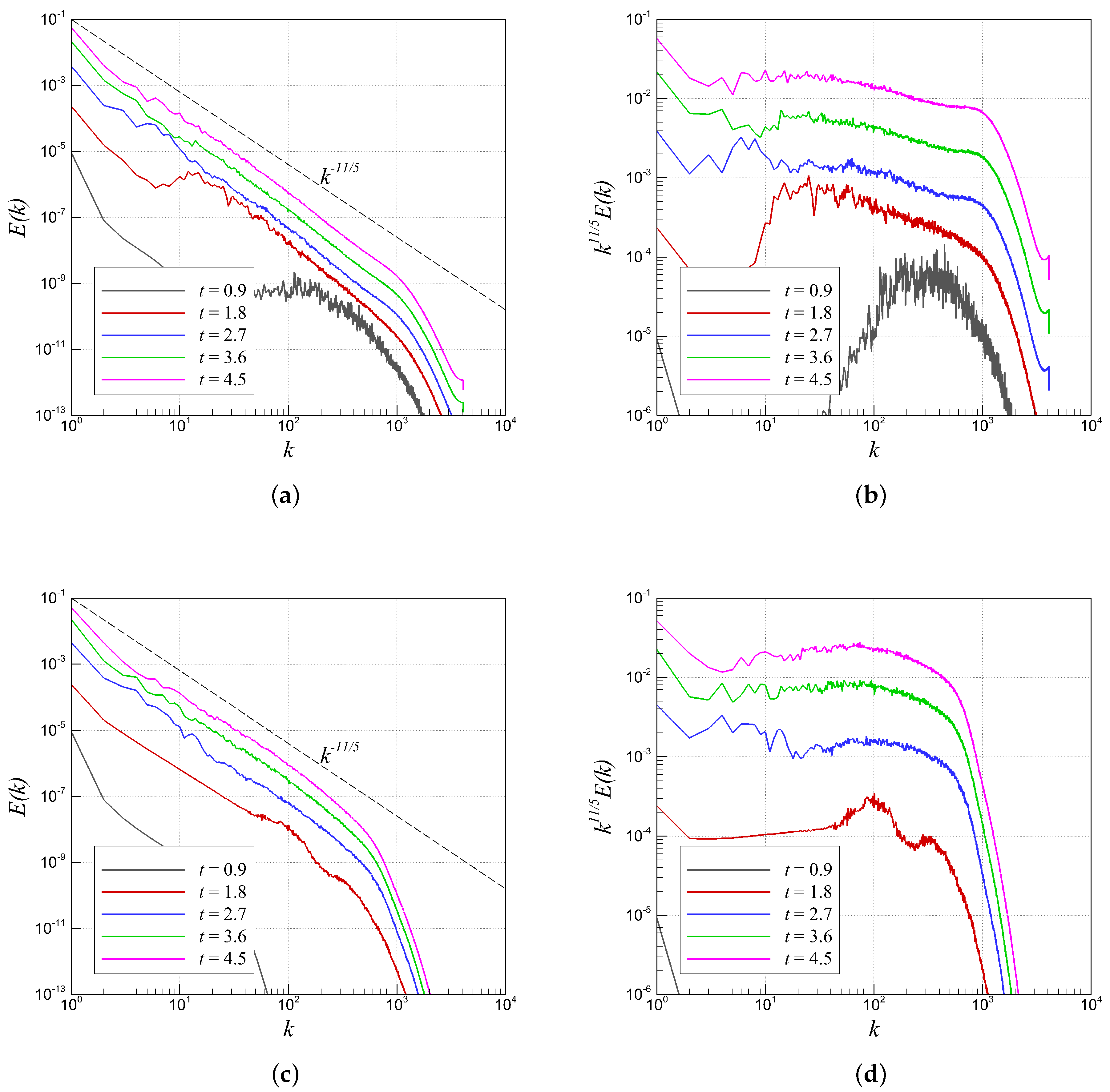
is set as in our case, and it is lower than , which indicates the formation of reacceleration phase in the flow field due to the secondary KH instabilities. As suggested in the literature [31], these secondary instabilities can be responsible for the change in the usual behavior of the spikes in single-mode RTI flows. These findings are also supported by the works of Liska and Wendroff [96] where they showed that the less dissipative schemes result in an interface break up while the instability might be suppressed by high dissipative schemes. The same observations can be found at final time in Figure 19 that the higher resolution results start to break the symmetry of the spike for both CS+RF schemes. However, the density fields obtained by the CS+RF and ILES schemes seem different due to different amount of dissipation added to the system by different solvers which would eventually lead to different evolution of the flow fields. To get a more precise understanding on the simulation results, we next focus on the density-weighted kinetic energy spectra plots. We can say from the time evolution of the kinetic energy spectra plot in Figure 20 that the trends of the spectra are similar at late-stage of the simulation. We can observe that the density-weighted spectra analysis for ILES-Roe scheme shows an inertial subrange following scaling law. On the other hand, the kinetic energy spectra for CS+RF scheme follow the scaling in Figure 21. To validate our findings further, we present the power density spectra plots for both ILES-Roe and CS+RF () schemes in Figure 22. The power density spectra display a good alignment with the reference line. Since the time evolution of the field for both schemes follow a similar trend, we can consider the solutions at final time for rest of our analysis.
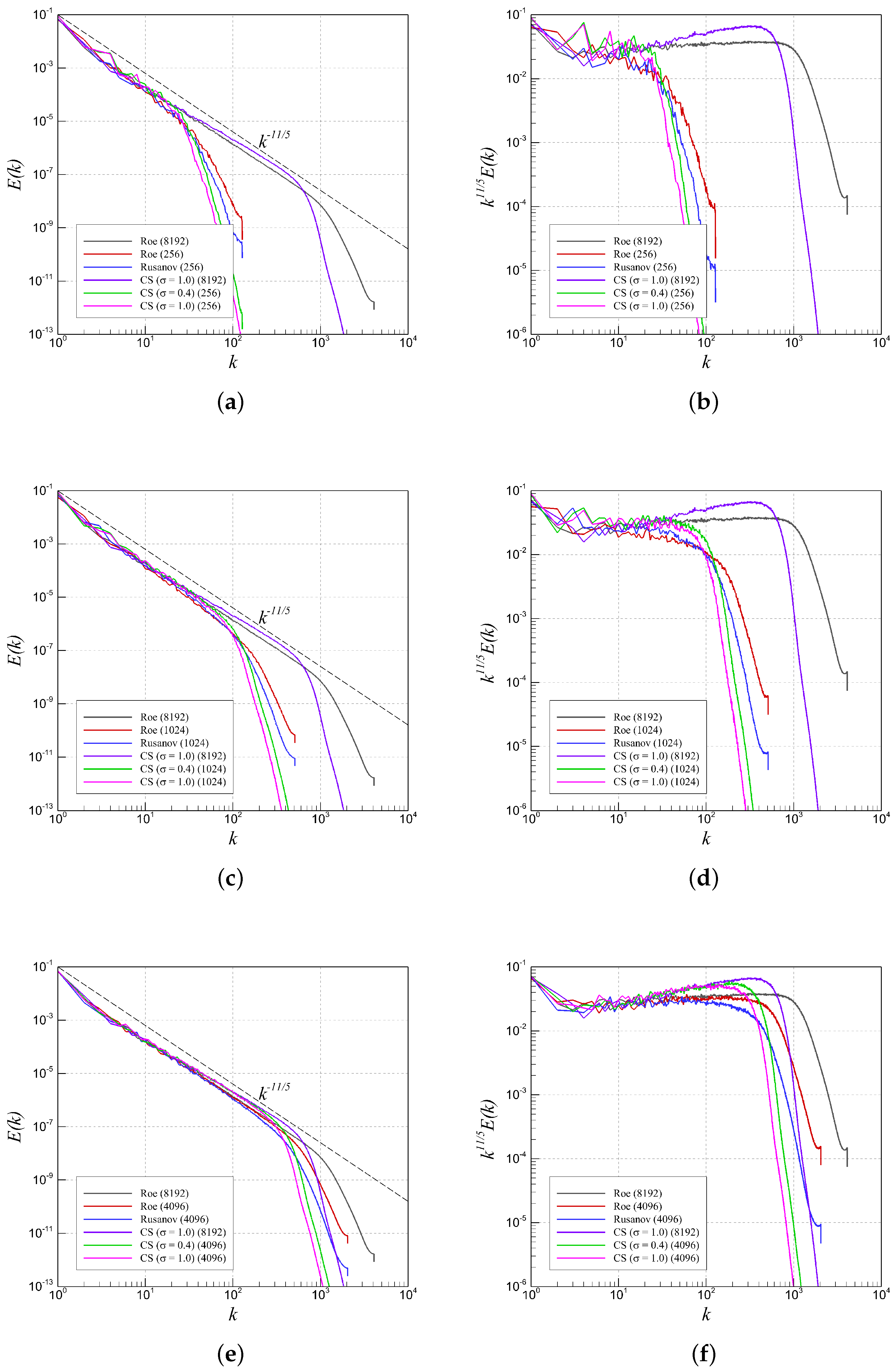
Figure 23 shows that the ILES-Rusanov solver is more dissipative than the ILES-Roe solver as expected and the CS+RF scheme with is more dissipative than the solver. One interesting point can be noticed that the density-weighted spectra for the CS+RF scheme tend to deviate from the reference line at high wavenumber; however, the kinetic energy spectra in Figure 24 and the density-weighted spectra in Figure 25 clearly show that the spectra for the CS+RF scheme follow the reference scaling laws. On the other hand, the ILES spectra also maintain the inertial subrange following the and laws. Finally, similar to the previous section of multi-mode RTI case, we find the CS+RF solver captures more scales in the inertial range than the ILES solvers as shown in Figure 26. However, the ILES solvers resolve more scales in the high wavenumber region. This explains the reason we have seen different density field evolution for different solvers and appearance of smaller scales in ILES solvers than the CS+RF solvers. Since the ILES-Roe solver is least dissipative among the other solvers, we can see in the density contour plots that the ILES-Roe solution deviates most from the symmetry.
5. Summary and Conclusions
In this paper, we put an effort to show the performance of a relaxation filtering approach using central scheme (CS+RF) on resolving the flows resulting from Rayleigh–Taylor hydrodynamic instability, and compare the simulation results with the results obtained by two common ILES-Riemann solver schemes. To assess the performance of the solvers, we use the density field contours and different spectra plots. We further analyze the resolution capacity of both CS+RF and ILES schemes as well as the flow nature at high-resolution simulation using CS+RF and ILES schemes. To validate the observations from the field plots, we use the statistical tools, i.e., kinetic energy and power density spectra plots for both high and coarse resolutions which show consistency with the existing results in the literature. In our investigation, we consider the two-dimensional RTI test problem with two different initial conditions. From the simulation results of both cases, we come to this conclusion that the CS+RF schemes capture more scales in the inertial subregion whereas the ILES schemes resolve a wide range of scales in high wavenumber region. The ILES-Rusanov scheme is more dissipative than the ILES-Roe scheme, and hence, the ILES-Roe scheme tends to deviate more from symmetry in the spike of single-mode RTI case. On the other hand, it is also observed that the dissipation can be controlled by parameter for CS+RF scheme which also affect the perturbation as well as the evolution of the flow field. Furthermore, we observe that the kinetic energy spectra follow scaling law for both multi-mode and single-mode RTI case whereas the power density spectra plots are seen to be more align to line at different resolutions. Also, we observe a chaotic mixing at late-time stage for single-mode RTI case at high resolution. It is because of the formation of secondary KH instabilities at high-resolution simulation of single-mode RTI case. The higher numerical dissipation due to the coarser resolution suppresses the formation of secondary instabilities which is the reason behind the preservation of symmetry for our coarse-resolution simulation results. Overall, we believe the study of relaxation filtering approach using CS will be a good contribution to the numerical study of RTI-induced flows as well as for understanding the nature of the flow field with the evolution of the instability.
Author Contributions
Conceptualization, O.S.; Data curation, S.M.R. and O.S.; Formal analysis, S.M.R. and O.S.; Visualization, S.M.R. and O.S.; Methodology, O.S.; Supervision, O.S.; Writing—original draft, S.M.R.; and Writing—review and editing, S.M.R. and O.S.
Funding
This research received no external funding.
Acknowledgments
The computing for this project was performed by using resources from the High-Performance Computing Center (HPCC) at Oklahoma State University.
Conflicts of Interest
The authors declare no conflict of interest.
References
- Taylor, G.I. The instability of liquid surfaces when accelerated in a direction perpendicular to their planes. I. Proc. R. Soc. Lond. Ser. Math. Phys. Sci. 1950, 201, 192–196. [Google Scholar]
- Cui, A.; Street, R.L. Large-eddy simulation of coastal upwelling flow. Environ. Fluid Mech. 2004, 4, 197–223. [Google Scholar] [CrossRef]
- Jevons, W.S., II. On the cirrous form of cloud. Lond. Edinburgh Dublin Philos. Mag. J. Sci. 1857, 14, 22–35. [Google Scholar] [CrossRef]
- Bradley, P. The effect of mix on capsule yields as a function of shell thickness and gas fill. Phys. Plasmas 2014, 21, 062703. [Google Scholar] [CrossRef]
- Bell, J.; Day, M.; Rendleman, C.; Woosley, S.; Zingale, M. Direct numerical simulations of type Ia supernovae flames. II. The Rayleigh-Taylor instability. Astrophys. J. 2004, 608, 883. [Google Scholar] [CrossRef]
- Hillebrandt, W.; Niemeyer, J.C. Type Ia supernova explosion models. Annu. Rev. Astron. Astrophys. 2000, 38, 191–230. [Google Scholar] [CrossRef]
- Racca, R.A.; Annett, C.H. Simple demonstration of Rayleigh-Taylor instability. Am. J. Phys. 1985, 53, 484–486. [Google Scholar] [CrossRef]
- Chertkov, M.; Lebedev, V.; Vladimirova, N. Reactive Rayleigh–Taylor turbulence. J. Fluid Mech. 2009, 633, 1–16. [Google Scholar] [CrossRef]
- Veynante, D.; Trouvé, A.; Bray, K.; Mantel, T. Gradient and counter-gradient scalar transport in turbulent premixed flames. J. Fluid Mech. 1997, 332, 263–293. [Google Scholar] [CrossRef]
- Petrasso, R.D. Rayleigh’s challenge endures. Nature 1994, 367, 217. [Google Scholar] [CrossRef]
- Lewis, D.J. The instability of liquid surfaces when accelerated in a direction perpendicular to their planes. II. Proc. R. Soc. Lond. Ser. Math. Phys. Sci. 1950, 202, 81–96. [Google Scholar]
- Lord, R. Investigation of the character of the equilibrium of an incompressible heavy fluid of variable density. Sci. Pap. 1900, 200–207. [Google Scholar]
- Zhou, Y. Rayleigh–Taylor and Richtmyer–Meshkov instability induced flow, turbulence, and mixing. I. Phys. Rep. 2017, 720–722, 1–136. [Google Scholar]
- Zhou, Y. Rayleigh–Taylor and Richtmyer–Meshkov instability induced flow, turbulence, and mixing. II. Phys. Rep. 2017, 723–725, 1–160. [Google Scholar] [CrossRef]
- Piriz, A.; Cortazar, O.; Lopez Cela, J.; Tahir, N. The Rayleigh-Taylor instability. Am. J. Phys. 2006, 74, 1095–1098. [Google Scholar] [CrossRef]
- Boffetta, G.; Mazzino, A. Incompressible Rayleigh–Taylor turbulence. Annu. Rev. Fluid Mech. 2017, 49, 119–143. [Google Scholar] [CrossRef]
- Sharp, D.H. Overview of Rayleigh-Taylor Instability; Technical Report; Los Alamos National Lab.: Los Alamos, NM, USA, 1983. [Google Scholar]
- Dimonte, G.; Youngs, D.; Dimits, A.; Weber, S.; Marinak, M.; Wunsch, S.; Garasi, C.; Robinson, A.; Andrews, M.; Ramaprabhu, P.; et al. A comparative study of the turbulent Rayleigh–Taylor instability using high-resolution three-dimensional numerical simulations: The Alpha-Group collaboration. Phys. Fluids 2004, 16, 1668–1693. [Google Scholar] [CrossRef]
- Mueschke, N.J.; Schilling, O. Investigation of Rayleigh–Taylor turbulence and mixing using direct numerical simulation with experimentally measured initial conditions. I. Comparison to experimental data. Phys. Fluids 2009, 21, 014106. [Google Scholar] [CrossRef]
- Wei, T.; Livescu, D. Late-time quadratic growth in single-mode Rayleigh-Taylor instability. Phys. Rev. E 2012, 86, 046405. [Google Scholar] [CrossRef]
- Dalziel, S.; Linden, P.; Youngs, D. Self-similarity and internal structure of turbulence induced by Rayleigh–Taylor instability. J. Fluid Mech. 1999, 399, 1–48. [Google Scholar] [CrossRef]
- Ristorcelli, J.; Clark, T. Rayleigh–Taylor turbulence: Self-similar analysis and direct numerical simulations. J. Fluid Mech. 2004, 507, 213–253. [Google Scholar] [CrossRef]
- Xin, J.; Yan, R.; Wan, Z.H.; Sun, D.J.; Zheng, J.; Zhang, H.; Aluie, H.; Betti, R. Two mode coupling of the ablative Rayleigh-Taylor instabilities. Phys. Plasmas 2019, 26, 032703. [Google Scholar] [CrossRef]
- Jun, B.I.; Norman, M.L.; Stone, J.M. A numerical study of Rayleigh-Taylor instability in magnetic fluids. Astrophys. J. 1995, 453, 332. [Google Scholar] [CrossRef]
- Cabot, W. Comparison of two-and three-dimensional simulations of miscible Rayleigh-Taylor instability. Phys. Fluids 2006, 18, 045101. [Google Scholar] [CrossRef]
- Anuchina, N.; Volkov, V.; Gordeychuk, V.; Es’ kov, N.; Ilyutina, O.; Kozyrev, O. Numerical simulations of Rayleigh–Taylor and Richtmyer–Meshkov instability using MAH-3 code. J. Comput. Appl. Math. 2004, 168, 11–20. [Google Scholar] [CrossRef]
- Zhao, D.; Aluie, H. Inviscid criterion for decomposing scales. Phys. Rev. Fluids 2018, 3, 054603. [Google Scholar] [CrossRef]
- Livescu, D.; Ristorcelli, J. Buoyancy-driven variable-density turbulence. J. Fluid Mech. 2007, 591, 43–71. [Google Scholar] [CrossRef]
- Kokkinakis, I.; Drikakis, D.; Youngs, D.; Williams, R. Two-equation and multi-fluid turbulence models for Rayleigh–Taylor mixing. Int. J. Heat Fluid Flow 2015, 56, 233–250. [Google Scholar] [CrossRef]
- Youngs, D. Large eddy simulation and 1D/2D engineering models for Rayleigh-Taylor mixing. In Proceedings of the IWPCTM: 12th International Workshop on the Physics of Compressible Turbulent Mixing, Moscow, Russia, 12–17 July 2010; pp. 12–17. [Google Scholar]
- Ramaprabhu, P.; Dimonte, G.; Woodward, P.; Fryer, C.; Rockefeller, G.; Muthuraman, K.; Lin, P.H.; Jayaraj, J. The late-time dynamics of the single-mode Rayleigh-Taylor instability. Phys. Fluids 2012, 24, 074107. [Google Scholar] [CrossRef]
- Glimm, J.; Li, X.l.; Lin, A.D. Nonuniform approach to terminal velocity for single mode Rayleigh-Taylor instability. Acta Math. Appl. Sin. 2002, 18, 1–8. [Google Scholar] [CrossRef]
- Daly, B.J. Numerical study of two fluid Rayleigh-Taylor instability. Phys. Fluids 1967, 10, 297–307. [Google Scholar] [CrossRef]
- Kane, J.; Arnett, D.; Remington, B.; Glendinning, S.; Bazán, G.; Müller, E.; Fryxell, B.; Teyssier, R. Two-dimensional versus three-dimensional supernova hydrodynamic instability growth. Astrophys. J. 2000, 528, 989. [Google Scholar] [CrossRef]
- Goncharov, V. Analytical model of nonlinear, single-mode, classical Rayleigh-Taylor instability at arbitrary Atwood numbers. Phys. Rev. Lett. 2002, 88, 134502. [Google Scholar] [CrossRef]
- Young, Y.N.; Tufo, H.; Dubey, A.; Rosner, R. On the miscible Rayleigh–Taylor instability: Two and three dimensions. J. Fluid Mech. 2001, 447, 377–408. [Google Scholar] [CrossRef]
- Youngs, D.L. Three-dimensional numerical simulation of turbulent mixing by Rayleigh–Taylor instability. Phys. Fluids A Fluid Dyn. 1991, 3, 1312–1320. [Google Scholar] [CrossRef]
- Youngs, D.L. Numerical simulation of mixing by Rayleigh–Taylor and Richtmyer–Meshkov instabilities. Laser Part. Beams 1994, 12, 725–750. [Google Scholar] [CrossRef]
- Shvarts, D.; Alon, U.; Ofer, D.; McCrory, R.; Verdon, C. Nonlinear evolution of multimode Rayleigh–Taylor instability in two and three dimensions. Phys. Plasmas 1995, 2, 2465–2472. [Google Scholar] [CrossRef]
- Oron, D.; Arazi, L.; Kartoon, D.; Rikanati, A.; Alon, U.; Shvarts, D. Dimensionality dependence of the Rayleigh–Taylor and Richtmyer–Meshkov instability late-time scaling laws. Phys. Plasmas 2001, 8, 2883–2889. [Google Scholar] [CrossRef]
- Zhou, Y. A scaling analysis of turbulent flows driven by Rayleigh–Taylor and Richtmyer–Meshkov instabilities. Phys. Fluids 2001, 13, 538–543. [Google Scholar] [CrossRef]
- Shvarts, D.; Oron, D.; Kartoon, D.; Rikanati, A.; Sadot, O.; Srebro, Y.; Yedvab, Y.; Ofer, D.; Levin, A.; Sarid, E.; et al. Scaling laws of nonlinear Rayleigh-Taylor and Richtmyer-Meshkov instabilities in two and three dimensions (IFSA 1999). In Edward Teller Lectures: Lasers and Inertial Fusion Energy; World Scientific: Singapore, 2016; pp. 253–260. [Google Scholar]
- Chertkov, M. Phenomenology of Rayleigh-Taylor turbulence. Phys. Rev. Lett. 2003, 91, 115001. [Google Scholar] [CrossRef]
- Celani, A.; Mazzino, A.; Vozella, L. Rayleigh-Taylor turbulence in two dimensions. Phys. Rev. Lett. 2006, 96, 134504. [Google Scholar] [CrossRef]
- Margolin, L. The reality of artificial viscosity. Shock Waves 2019, 29, 27–35. [Google Scholar] [CrossRef]
- Brehm, C.; Barad, M.F.; Housman, J.A.; Kiris, C.C. A comparison of higher-order finite-difference shock capturing schemes. Comput. Fluids 2015, 122, 184–208. [Google Scholar] [CrossRef]
- Margolin, L.G.; Rider, W.J.; Grinstein, F.F. Modeling turbulent flow with implicit LES. J. Turbul. 2006, 7, N15. [Google Scholar] [CrossRef]
- Zhou, Y.; Thornber, B. A comparison of three approaches to compute the effective Reynolds number of the implicit large-eddy simulations. J. Fluids Eng. 2016, 138, 070905. [Google Scholar] [CrossRef]
- Maulik, R.; San, O. Resolution and energy dissipation characteristics of implicit LES and explicit filtering models for compressible turbulence. Fluids 2017, 2, 14. [Google Scholar] [CrossRef]
- San, O.; Kara, K. Numerical assessments of high-order accurate shock capturing schemes: Kelvin–Helmholtz type vortical structures in high-resolutions. Comput. Fluids 2014, 89, 254–276. [Google Scholar] [CrossRef]
- Titarev, V.A.; Toro, E.F. Finite-volume WENO schemes for three-dimensional conservation laws. J. Comput. Phys. 2004, 201, 238–260. [Google Scholar] [CrossRef]
- Pirozzoli, S. Numerical methods for high-speed flows. Annu. Rev. Fluid Mech. 2011, 43, 163–194. [Google Scholar] [CrossRef]
- Brehm, C. On consistent boundary closures for compact finite-difference WENO schemes. J. Comput. Phys. 2017, 334, 573–581. [Google Scholar] [CrossRef]
- Wong, M.L.; Lele, S.K. High-order localized dissipation weighted compact nonlinear scheme for shock-and interface-capturing in compressible flows. J. Comput. Phys. 2017, 339, 179–209. [Google Scholar] [CrossRef]
- Zhao, S.; Lardjane, N.; Fedioun, I. Comparison of improved finite-difference WENO schemes for the implicit large eddy simulation of turbulent non-reacting and reacting high-speed shear flows. Comput. Fluids 2014, 95, 74–87. [Google Scholar] [CrossRef]
- Hu, X.; Wang, Q.; Adams, N.A. An adaptive central-upwind weighted essentially non-oscillatory scheme. J. Comput. Phys. 2010, 229, 8952–8965. [Google Scholar] [CrossRef]
- Mathew, J.; Foysi, H.; Friedrich, R. A new approach to LES based on explicit filtering. Int. J. Heat Fluid Flow 2006, 27, 594–602. [Google Scholar] [CrossRef]
- Lund, T. The use of explicit filters in large eddy simulation. Comput. Math. Appl. 2003, 46, 603–616. [Google Scholar] [CrossRef]
- Berland, J.; Lafon, P.; Daude, F.; Crouzet, F.; Bogey, C.; Bailly, C. Filter shape dependence and effective scale separation in large-eddy simulations based on relaxation filtering. Comput. Fluids 2011, 47, 65–74. [Google Scholar] [CrossRef]
- Bose, S.T.; Moin, P.; You, D. Grid-independent large-eddy simulation using explicit filtering. Phys. Fluids 2010, 22, 105103. [Google Scholar] [CrossRef]
- Vasilyev, O.V.; Lund, T.S.; Moin, P. A general class of commutative filters for LES in complex geometries. J. Comput. Phys. 1998, 146, 82–104. [Google Scholar] [CrossRef]
- San, O. Analysis of low-pass filters for approximate deconvolution closure modelling in one-dimensional decaying Burgers turbulence. Int. J. Comput. Fluid Dyn. 2016, 30, 20–37. [Google Scholar] [CrossRef]
- Najafi-Yazdi, A.; Najafi-Yazdi, M.; Mongeau, L. A high resolution differential filter for large eddy simulation: Toward explicit filtering on unstructured grids. J. Comput. Phys. 2015, 292, 272–286. [Google Scholar] [CrossRef]
- Shivamoggi, B.K. Spectral laws for the compressible isotropic turbulence. In Instability, Transition, and Turbulence; Springer: New York, NY, USA, 1992; pp. 524–534. [Google Scholar]
- Shivamoggi, B.K. Multi-fractal aspects of the fine-scale structure of temperature fluctuations in isotropic turbulence. Phys. A Stat. Mech. Its Appl. 1995, 221, 460–477. [Google Scholar] [CrossRef]
- Shivamoggi, B.K. Intermittency in the enstrophy cascade of two-dimensional fully developed turbulence: Universal features. Ann. Phys. 2008, 323, 444–460. [Google Scholar] [CrossRef]
- Shivamoggi, B. Compressible turbulence: Multi-fractal scaling in the transition to the dissipative regime. Phys. A Stat. Mech. Its Appl. 2011, 390, 1534–1538. [Google Scholar] [CrossRef]
- Sun, B. The temporal scaling laws of compressible turbulence. Mod. Phys. Lett. B 2016, 30, 1650297. [Google Scholar] [CrossRef]
- Sun, B. Scaling laws of compressible turbulence. Appl. Math. Mech. 2017, 38, 765–778. [Google Scholar] [CrossRef]
- Parent, B. Positivity-preserving high-resolution schemes for systems of conservation laws. J. Comput. Phys. 2012, 231, 173–189. [Google Scholar] [CrossRef]
- Gottlieb, S.; Shu, C.W. Total variation diminishing Runge-Kutta schemes. Math. Comput. Am. Math. Soc. 1998, 67, 73–85. [Google Scholar] [CrossRef]
- Godunov, S.K. A difference method for numerical calculation of discontinuous solutions of the equations of hydrodynamics. Mat. Sb. 1959, 89, 271–306. [Google Scholar]
- Grinstein, F.F.; Margolin, L.G.; Rider, W.J. Implicit Large Eddy Simulation: Computing Turbulent Fluid Dynamics; Cambridge University Press: New York, NY, USA, 2007. [Google Scholar]
- Denaro, F.M. What does finite volume-based implicit filtering really resolve in large-eddy simulations? J. Comput. Phys. 2011, 230, 3849–3883. [Google Scholar] [CrossRef]
- Liu, X.D.; Osher, S.; Chan, T. Weighted essentially non-oscillatory schemes. J. Comput. Phys. 1994, 115, 200–212. [Google Scholar] [CrossRef]
- Harten, A.; Engquist, B.; Osher, S.; Chakravarthy, S.R. Uniformly high order accurate essentially non-oscillatory schemes, III. In Upwind and High-Resolution Schemes; Springer: New York, NY, USA, 1987; pp. 218–290. [Google Scholar]
- Shu, C.W.; Osher, S. Efficient implementation of essentially non-oscillatory shock-capturing schemes. J. Comput. Phys. 1988, 77, 439–471. [Google Scholar] [CrossRef]
- Jiang, G.S.; Shu, C.W. Efficient implementation of weighted ENO schemes. J. Comput. Phys. 1996, 126, 202–228. [Google Scholar] [CrossRef]
- Henrick, A.K.; Aslam, T.D.; Powers, J.M. Mapped weighted essentially non-oscillatory schemes: Achieving optimal order near critical points. J. Comput. Phys. 2005, 207, 542–567. [Google Scholar] [CrossRef]
- Borges, R.; Carmona, M.; Costa, B.; Don, W.S. An improved weighted essentially non-oscillatory scheme for hyperbolic conservation laws. J. Comput. Phys. 2008, 227, 3191–3211. [Google Scholar] [CrossRef]
- Roe, P.L. Approximate Riemann solvers, parameter vectors, and difference schemes. J. Comput. Phys. 1981, 43, 357–372. [Google Scholar] [CrossRef]
- Harten, A. High resolution schemes for hyperbolic conservation laws. J. Comput. Phys. 1983, 49, 357–393. [Google Scholar] [CrossRef]
- Rusanov, V.V. The calculation of the interaction of non-stationary shock waves with barriers. Zhurnal Vychislitel’Noi Mat. Mat. Fiz. 1961, 1, 267–279. [Google Scholar]
- Lax, P.D. Weak solutions of nonlinear hyperbolic equations and their numerical computation. Commun. Pure Appl. Math. 1954, 7, 159–193. [Google Scholar] [CrossRef]
- Toro, E.F. Riemann Solvers and Numerical Methods for Fluid Dynamics: A Practical Introduction; Springer Science & Business Media: Berlin, Germany, 2013. [Google Scholar]
- Hyman, J.M.; Knapp, R.J.; Scovel, J.C. High order finite volume approximations of differential operators on nonuniform grids. Phys. D Nonlinear Phenom. 1992, 60, 112–138. [Google Scholar] [CrossRef]
- Fauconnier, D.; Bogey, C.; Dick, E. On the performance of relaxation filtering for large-eddy simulation. J. Turbul. 2013, 14, 22–49. [Google Scholar] [CrossRef]
- Bogey, C.; Bailly, C. Computation of a high Reynolds number jet and its radiated noise using large eddy simulation based on explicit filtering. Comput. Fluids 2006, 35, 1344–1358. [Google Scholar] [CrossRef]
- Bull, J.R.; Jameson, A. Explicit filtering and exact reconstruction of the sub-filter stresses in large eddy simulation. J. Comput. Phys. 2016, 306, 117–136. [Google Scholar] [CrossRef]
- San, O. A dynamic eddy-viscosity closure model for large eddy simulations of two-dimensional decaying turbulence. Int. J. Comput. Fluid Dyn. 2014, 28, 363–382. [Google Scholar] [CrossRef]
- Gropp, W.; Lusk, E.; Doss, N.; Skjellum, A. A high-performance, portable implementation of the MPI message passing interface standard. Parallel Comput. 1996, 22, 789–828. [Google Scholar] [CrossRef]
- Gropp, W.D.; Gropp, W.; Lusk, E.; Skjellum, A.; Lusk, E. Using MPI: Portable Parallel Programming with the Message-Passing Interface; MIT Press: Cambridge, MA, USA, 1999; Volume 1. [Google Scholar]
- Banerjee, A.; Andrews, M.J. 3D simulations to investigate initial condition effects on the growth of Rayleigh–Taylor mixing. Int. J. Heat Mass Transf. 2009, 52, 3906–3917. [Google Scholar] [CrossRef]
- Vladimirova, N.; Chertkov, M. Self-similarity and universality in Rayleigh–Taylor, Boussinesq turbulence. Phys. Fluids 2009, 21, 015102. [Google Scholar] [CrossRef]
- Xu, Z.; Duo-Wang, T. Direct Numerical Simulation of the Rayleigh- Taylor Instability with the Spectral Element Method. Chin. Phys. Lett. 2009, 26, 084703. [Google Scholar] [CrossRef]
- Liska, R.; Wendroff, B. Comparison of several difference schemes on 1D and 2D test problems for the Euler equations. Siam J. Sci. Comput. 2003, 25, 995–1017. [Google Scholar] [CrossRef]
- Stone, J.M.; Gardiner, T.A.; Teuben, P.; Hawley, J.F.; Simon, J.B. Athena: A new code for astrophysical MHD. Astrophys. Suppl. Ser. 2008, 178, 137–177. [Google Scholar] [CrossRef]
- Poinsot, T.J.; Lele, S.K. Boundary conditions for direct simulations of compressible viscous flows. J. Comput. Phys. 1992, 101, 104–129. [Google Scholar] [CrossRef]
- Youngs, D.L. Rayleigh–Taylor mixing: Direct numerical simulation and implicit large eddy simulation. Phys. Scr. 2017, 92, 074006. [Google Scholar] [CrossRef]
- San, O.; Kara, K. Evaluation of Riemann flux solvers for WENO reconstruction schemes: Kelvin–Helmholtz instability. Comput. Fluids 2015, 117, 24–41. [Google Scholar] [CrossRef]
- Lele, S.K. Compressibility effects on turbulence. Annu. Rev. Fluid Mech. 1994, 26, 211–254. [Google Scholar] [CrossRef]
- Kritsuk, A.G.; Norman, M.L.; Padoan, P.; Wagner, R. The statistics of supersonic isothermal turbulence. Astrophys. J. 2007, 665, 416. [Google Scholar] [CrossRef]
- Aluie, H. Scale decomposition in compressible turbulence. Phys. D Nonlinear Phenom. 2013, 247, 54–65. [Google Scholar] [CrossRef]
- San, O.; Maulik, R. Stratified Kelvin–Helmholtz turbulence of compressible shear flows. Nonlinear Process. Geophys. 2018, 25. [Google Scholar] [CrossRef]
- Press, W.H.; Teukolsky, S.A.; Vetterling, W.T.; Flannery, B.P. Numerical Recipes in FORTRAN: The Art of Scientific Computing, 2nd ed.; Cambridge University Press: New York, NY, USA, 1992. [Google Scholar]
- Kida, S.; Orszag, S.A. Energy and spectral dynamics in forced compressible turbulence. J. Sci. Comput. 1990, 5, 85–125. [Google Scholar] [CrossRef]
- Bolgiano, R., Jr. Turbulent spectra in a stably stratified atmosphere. J. Geophys. Res. 1959, 64, 2226–2229. [Google Scholar] [CrossRef]
- Livescu, D.; Wei, T.; Petersen, M. Direct Numerical Simulations of Rayleigh-Taylor Instability; Conference Series; IOP Publishing: Bristol, UK, 2011; Volume 318, p. 082007. [Google Scholar]
- Youngs, D.L. Numerical simulation of turbulent mixing by Rayleigh-Taylor instability. Phys. D Nonlinear Phenom. 1984, 12, 32–44. [Google Scholar] [CrossRef]
- Ramaprabhu, P.; Dimonte, G.; Andrews, M. A numerical study of the influence of initial perturbations on the turbulent Rayleigh–Taylor instability. J. Fluid Mech. 2005, 536, 285–319. [Google Scholar] [CrossRef]
- Shadloo, M.; Zainali, A.; Yildiz, M. Simulation of single mode Rayleigh–Taylor instability by SPH method. Comput. Mech. 2013, 51, 699–715. [Google Scholar] [CrossRef]
- Lee, H.G.; Kim, K.; Kim, J. On the long time simulation of the Rayleigh–Taylor instability. Int. J. Numer. Methods Eng. 2011, 85, 1633–1647. [Google Scholar] [CrossRef]
- Livescu, D.; Ristorcelli, J.; Petersen, M.; Gore, R. New phenomena in variable-density Rayleigh–Taylor turbulence. Phys. Scr. 2010, 2010, 014015. [Google Scholar] [CrossRef]
- Shi, J.; Zhang, Y.T.; Shu, C.W. Resolution of high order WENO schemes for complicated flow structures. J. Comput. Phys. 2003, 186, 690–696. [Google Scholar] [CrossRef]
- Fu, L.; Hu, X.Y.; Adams, N.A. A family of high-order targeted ENO schemes for compressible-fluid simulations. J. Comput. Phys. 2016, 305, 333–359. [Google Scholar] [CrossRef]
- Latini, M.; Schilling, O.; Don, W.S. Effects of WENO flux reconstruction order and spatial resolution on reshocked two-dimensional Richtmyer–Meshkov instability. J. Comput. Phys. 2007, 221, 805–836. [Google Scholar] [CrossRef]
- Tritschler, V.; Hu, X.; Hickel, S.; Adams, N. Numerical simulation of a Richtmyer–Meshkov instability with an adaptive central-upwind sixth-order WENO scheme. Phys. Scr. 2013, 2013, 014016. [Google Scholar] [CrossRef]
Figure 1.
Computational domain and initial conditions for the (a) multi-mode and (b) single-mode Rayleigh–Taylor instability (RTI) test case. Please note that we apply periodic boundary condition on left and right boundaries, and reflective boundary condition on top and bottom boundaries.
Figure 1.
Computational domain and initial conditions for the (a) multi-mode and (b) single-mode Rayleigh–Taylor instability (RTI) test case. Please note that we apply periodic boundary condition on left and right boundaries, and reflective boundary condition on top and bottom boundaries.

Figure 2.
Illustration of the periodic boundary condition (left and right boundaries) and the reflective boundary condition (top and bottom boundaries) on an arbitrary two-dimensional domain.
Figure 2.
Illustration of the periodic boundary condition (left and right boundaries) and the reflective boundary condition (top and bottom boundaries) on an arbitrary two-dimensional domain.

Figure 3.
Time evolution of density field for the RTI problem with multi-mode perturbation: (a) ; (b) ; (c) ; (d) . Results are obtained by the ILES-Roe scheme at a resolution of .
Figure 3.
Time evolution of density field for the RTI problem with multi-mode perturbation: (a) ; (b) ; (c) ; (d) . Results are obtained by the ILES-Roe scheme at a resolution of .

Figure 4.
Density contours for the RTI problem with multi-mode perturbation at for different coarse grid resolutions and ILES schemes: (a) ILES-Rusanov with resolution; (b) ILES-Rusanov with resolution; (c) ILES-Rusanov with resolution; (d) ILES-Roe with resolution; (e) ILES-Roe with resolution; (f) ILES-Roe with resolution. The gravity is directed in a vertically downward direction.

Figure 5.
Density contours for the RTI problem with multi-mode perturbation at for different coarse grid resolutions and filtering strength, of CS+RF schemes: (a) with resolution; (b) with resolution; (c) with resolution; (d) with resolution; (e) with resolution; (f) with resolution. The gravity is directed in a vertically downward direction.

Figure 6.
Time evolution of density-weighted kinetic energy spectra and compensated density-weighted kinetic energy spectra for the RTI problem with multi-mode perturbation obtained using different modeling approaches at a resolution of ; (a) density-weighted spectra using ILES-Roe solver; (b) compensated density-weighted spectra using ILES-Roe solver; (c) density-weighted spectra using CS+RF () solver; (d) compensated density-weighted spectra using CS+RF () solver.

Figure 7.
Time evolution of kinetic energy spectra and compensated kinetic energy spectra for the RTI problem with multi-mode perturbation obtained using different modeling approaches at a resolution of ; (a) kinetic energy spectra using ILES-Roe solver; (b) compensated kinetic energy spectra using ILES-Roe solver; (c) kinetic energy spectra using CS+RF () solver; (d) compensated kinetic energy spectra using CS+RF () solver.

Figure 8.
Time evolution of power density spectra and compensated power density spectra for the RTI problem with multi-mode perturbation obtained using different modeling approaches at a resolution of ; (a) power density spectra using ILES-Roe solver; (b) compensated power density spectra using ILES-Roe solver; (c) power density spectra using CS+RF () solver; (d) compensated power density spectra using CS+RF () solver.

Figure 9.
Comparison of ILES (ILES-Roe and ILES-Rusanov) models and CS+RF ( and ) models for the RTI problem with multi-mode perturbation showing the density-weighted kinetic energy spectra and compensated density-weighted kinetic energy spectra at different resolutions; (a) density-weighted spectra using ILES solvers; (b) compensated density-weighted spectra using ILES solvers; (c) density-weighted spectra using CS+RF solvers; (d) compensated density-weighted spectra using CS+RF solvers.

Figure 10.
Comparison of ILES (ILES-Roe and ILES-Rusanov) models and CS+RF ( and ) models for the RTI problem with multi-mode perturbation showing the kinetic energy spectra and compensated kinetic energy spectra at different resolutions; (a) kinetic energy spectra using ILES solvers; (b) compensated kinetic energy spectra using ILES solvers; (c) kinetic energy spectra using CS+RF solvers; (d) compensated kinetic energy spectra using CS+RF solvers.

Figure 11.
Comparison of ILES (ILES-Roe and ILES-Rusanov) models and CS+RF ( and ) models for the RTI problem with multi-mode perturbation showing the power density spectra and compensated power density spectra at different resolutions; (a) power density spectra using ILES solvers; (b) compensated power density spectra using ILES solvers; (c) power density spectra using CS+RF solvers; (d) compensated power density spectra using CS+RF solvers.

Figure 12.
Comparison between ILES and CS+RF models for the RTI problem with multi-mode perturbation at different resolutions; (a) density-weighted spectra at resolution; (b) compensated density-weighted spectra at resolution; (c) density-weighted spectra at resolution; (d) compensated density-weighted spectra at resolution; (e) density-weighted spectra at resolution; (f) compensated density-weighted spectra at resolution.

Figure 13.
Time evolution of density field for the RTI problem with single-mode perturbation: (a) ; (b) ; (c) ; (d) . Results are obtained by the ILES-Roe scheme at a resolution of .
Figure 13.
Time evolution of density field for the RTI problem with single-mode perturbation: (a) ; (b) ; (c) ; (d) . Results are obtained by the ILES-Roe scheme at a resolution of .

Figure 14.
Time evolution of density field for the RTI problem with single-mode perturbation for different coarse grid resolutions using ILES-Rusanov scheme: (a) ILES-Rusanov with resolution at ; (b) ILES-Rusanov with resolution at ; and (c) ILES-Rusanov with resolution at ; (d) ILES-Rusanov with resolution at ; (e) ILES-Rusanov with resolution at ; and (f) ILES-Rusanov with resolution at . The gravity is directed in a vertically downward direction.

Figure 15.
Time evolution of density field for the RTI problem with single-mode perturbation for different coarse grid resolutions using ILES-Roe scheme: (a) ILES-Roe with resolution at ; (b) ILES-Roe with resolution at ; and (c) ILES-Roe with resolution at ; (d) ILES-Roe with resolution at ; (e) ILES-Roe with resolution at ; and (f) ILES-Roe with resolution at . The gravity is directed in a vertically downward direction.

Figure 16.
Time evolution of density field for the RTI problem with single-mode perturbation for different coarse grid resolutions using CS+RF scheme (): (a) CS+RF scheme () with resolution at ; (b) CS+RF scheme () with resolution at ; and (c) CS+RF scheme () with resolution at ; (d) CS+RF scheme () with resolution at ; (e) CS+RF scheme () with resolution at ; and (f) CS+RF scheme () with resolution at . The gravity is directed in a vertically downward direction.

Figure 17.
Time evolution of density field for the RTI problem with single-mode perturbation for different coarse grid resolutions using CS+RF scheme (): (a) CS+RF scheme () with resolution at ; (b) CS+RF scheme () with resolution at ; and (c) CS+RF scheme () with resolution at ; (d) CS+RF scheme () with resolution at ; (e) CS+RF scheme () with resolution at ; and (f) CS+RF scheme () with resolution at . The gravity is directed in a vertically downward direction.

Figure 18.
Density contours for the RTI problem with single-mode perturbation at for different coarse grid resolutions and ILES schemes: (a) ILES-Rusanov with resolution; (b) ILES-Rusanov with resolution; (c) ILES-Rusanov with resolution; (d) ILES-Roe with resolution; (e) ILES-Roe with resolution; (f) ILES-Roe with resolution. The gravity is directed in a vertically downward direction.

Figure 19.
Density contours for the RTI problem with single-mode perturbation at for different coarse grid resolutions and filtering strength, of CS+RF schemes: (a) with resolution; (b) with resolution; (c) with resolution; (d) with resolution; (e) with resolution; (f) with resolution. The gravity is directed in a vertically downward direction.

Figure 20.
Time evolution of density-weighted kinetic energy spectra and compensated density-weighted kinetic energy spectra for the RTI problem with single-mode perturbation obtained using different modeling approaches at a resolution of ; (a) density-weighted spectra using ILES-Roe solver; (b) compensated density-weighted spectra using ILES-Roe solver; (c) density-weighted spectra using CS+RF () solver; (d) compensated density-weighted spectra using CS+RF () solver.

Figure 21.
Time evolution of kinetic energy spectra and compensated kinetic energy spectra for the RTI problem with single-mode perturbation obtained using different modeling approaches at a resolution of ; (a) kinetic energy spectra using ILES-Roe solver; (b) compensated kinetic energy spectra using ILES-Roe solver; (c) kinetic energy spectra using CS+RF () solver; (d) compensated kinetic energy spectra using CS+RF () solver.

Figure 22.
Time evolution of power density spectra and compensated power density spectra for the RTI problem with single-mode perturbation obtained using different modeling approaches at a resolution of ; (a) power density spectra using ILES-Roe solver; (b) compensated power density spectra using ILES-Roe solver; (c) power density spectra using CS+RF () solver; (d) compensated power density spectra using CS+RF () solver.

Figure 23.
Comparison of ILES (ILES-Roe and ILES-Rusanov) models and CS+RF ( and ) models at different resolutions for the RTI problem with single-mode perturbation showing the density-weighted kinetic energy spectra and compensated density-weighted kinetic energy spectra; (a) density-weighted spectra using ILES solvers; (b) compensated density-weighted spectra using ILES solvers; (c) density-weighted spectra using CS+RF solvers; (d) compensated density-weighted spectra using CS+RF solvers.

Figure 24.
Comparison of ILES (ILES-Roe and ILES-Rusanov) models and CS+RF ( and ) models at different resolutions for the RTI problem with single-mode perturbation showing the kinetic energy spectra and compensated kinetic energy spectra; (a) kinetic energy spectra using ILES solvers; (b) compensated kinetic energy spectra using ILES solvers; (c) kinetic energy spectra using CS+RF solvers; (d) compensated kinetic energy spectra using CS+RF solvers.

Figure 25.
Comparison of ILES (ILES-Roe and ILES-Rusanov) models and CS+RF ( and ) models at different resolutions for the RTI problem with single-mode perturbation showing the power density spectra and compensated power density spectra; (a) power density spectra using ILES solvers; (b) compensated power density spectra using ILES solvers; (c) power density spectra using CS+RF solvers; (d) compensated power density spectra using CS+RF solvers.

Figure 26.
Comparison between ILES and CS+RF models for the RTI problem with single-mode perturbation at different resolutions; (a) density-weighted spectra at resolution; (b) compensated density-weighted spectra at resolution; (c) density-weighted spectra at resolution; (d) compensated density-weighted spectra at resolution; (e) density-weighted spectra at resolution; (f) compensated density-weighted spectra at resolution.

© 2019 by the authors. Licensee MDPI, Basel, Switzerland. This article is an open access article distributed under the terms and conditions of the Creative Commons Attribution (CC BY) license (http://creativecommons.org/licenses/by/4.0/).
Share and Cite
MDPI and ACS Style
Rahman, S.M.; San, O. A Relaxation Filtering Approach for Two-Dimensional Rayleigh–Taylor Instability-Induced Flows. Fluids 2019, 4, 78. https://doi.org/10.3390/fluids4020078
AMA Style
Rahman SM, San O. A Relaxation Filtering Approach for Two-Dimensional Rayleigh–Taylor Instability-Induced Flows. Fluids. 2019; 4(2):78. https://doi.org/10.3390/fluids4020078
Chicago/Turabian StyleRahman, Sk. Mashfiqur, and Omer San. 2019. "A Relaxation Filtering Approach for Two-Dimensional Rayleigh–Taylor Instability-Induced Flows" Fluids 4, no. 2: 78. https://doi.org/10.3390/fluids4020078