A Correction and Discussion on Log-Normal Intermittency B-Model


1
Department of Ocean Sciences, Tokyo University of Marine Science and Technology, 4-5-7 Konan, Minato-ku, Tokyo 108-8477, Japan
2
CNRS, Univ. Lille, Univ. Littoral Côte d’Opale, UMR 8187, LOG, Laboratoire d’Océanologie et de Géosciences, F 62930 Wimereux, France
*
Author to whom correspondence should be addressed.
Fluids 2019, 4(1), 35; https://doi.org/10.3390/fluids4010035
Submission received: 2 December 2018
/
Revised: 28 January 2019
/
Accepted: 13 February 2019
/
Published: 21 February 2019
(This article belongs to the Special Issue Multiscale Turbulent Transport)
Abstract
:This paper discusses a turbulent intermittency model introduced in 1990, the B-model. It was found that the original manuscript which introduced the B-model contained a couple arithmetic errors in the equations. This work goes over corrections to the original equations, and explains where problems arose in the derivations. These corrections cause the results to differ from those in the original manuscript, and these differences are discussed. A generalization of this B-model is then introduced to explore the range of behaviors this style of model provides. To distinguish between the different intermittency models discussed in this paper requires structure function power exponents of order greater than 12. As a source of comparison, data from a flume experiment is introduced, and, with the corrections introduced, this data seems to imply that an intermittency coefficient between and gives good agreement. Higher quality future measurements of high order moments could help with distinguishing the different intermittency models.
1. Introduction
Fluid turbulence is a phenomenon characterized by the presence of small scale fluctuations in the velocity and pressure fields, along with an increased rate of mixing of mass and momentum [1]. Turbulent flows also exhibit characteristic phenomena like coherent structures in the flow and intermittency. As the analytic and numerical solution of such flows is expensive and susceptible to chaos, one has to rely on models to simulate and simplify their dynamics. Such turbulence models include two-equation models (like the k- model and k- model [2]), Reynolds stress models (like the Speziale–Sarkar–Gatski model [3] and the Mishra–Girimaji model [4]), along with models in Large Eddy Simulations [5]. The B-model is an improvement on the log-normal model for the pdf of the dissipation rate in turbulent flows.
The first aim of this paper is to discuss the B-model introduced in the paper “Breakage models: lognormality and intermittency” [6] (hereinafter referred to as Y90) which introduces a model of turbulent intermittency, and to identify some errors in the original manuscript. We go over these corrections to the original equations and in Section 2.3 explain where the errors occurred. Originally, the Y90 model only considered the beta function for the distribution of the intermittency coefficient. A generalization of this model to any probability density function (pdf) is introduced in Section 2.4 to probe the range of behaviours this style of model provides. The model corrections cause the results to differ from those in the original manuscript. These differences are discussed in Section 4. This section also gives a brief discussion of the differences existing between the discrete B-model and the phenomenologically more realistic family of continuous cascade models.
2. Breakage Models
Turbulence obeys the Navier–Stokes equation. When fluid flow is at a low Reynolds number, the Navier–Stokes equation can predict the flow since nonlinear terms are not dominant. As the Reynolds number increases, the nonlinear terms in the Navier–Stokes equation create chaotic flow. However, the flow exhibits coherent structures at fully developed turbulence, which can only be dealt with in the statistical sense. As stressed by Frisch [7] in his seminal work on the stochastic nature of turbulence, “the understanding of chaos in deterministic systems gives us confidence that a probabilistic description of turbulence is justified”. As a matter of fact, Kolmogorov [8] is the most successful statistical description of fully developed turbulence and is the root of intermittency models. Turbulent intermittency is the phenomenon where the instantaneous dissipation rate intermittently reaches very high values, and more often as the Reynolds number increases. An introduction to turbulent intermittency can be found in Frisch [9].
2.1. The Gurvich–Yaglom Model
Gurvich & Yaglom [10] (hereinafter referred to as GY) derived a theory of log-normality for the dissipation rate (the rate at which turbulent kinetic energy dissipates), extending the model of Kolmogorov [8]. Here, we explain parts of the GY model that are relevant to the Y90 paper and our discussion.
The GY model applied a breakage cascade to study how the statistics of turbulent fluctuations vary with the length scale under consideration. In this model, the average dissipation rate over some spatial domain Q is
In this equation, the instantaneous local dissipation rate is given by
where is viscosity and are the strain rates, defined from the fluid velocity u as
Here, both the turbulent velocities and spatial coordinates are components of 3D vectors, with being shorthand for the whole vector itself.
The original spatial domain Q is then divided into successively smaller subdomains with average dissipation rate in this subdomain given by a random variable ,
The breakage coefficient is then defined as the ratio of two successive dissipation rates ,
where is the number of breakage processes. Given this relation, conservation of energy demands that the expected ratio of two successive dissipation rates must be 1,
The length scale of a given subdomain is represented by . In the GY model, the ratio of successive length scales is constant,
This breakage process is taken to continue until the length scale where fluctuations of can be neglected. We also define the largest length scale as L, and the smallest scale at which fluctuations can be neglected as .
Using the above notation, the dissipation rates can be written as (noting that , the expectation value of the dissipation rate over the whole spatial domain)
where is the value of in the domain . Using the central limit theorem, Gurvich & Yaglom [10] then argue that both and are normally distributed, and hence and are log-normally distributed. The means and variances are denoted
Next, because the summands , beyond the first ones, are identically distributed, the above variables may be represented as
where
The terms A and come from the non-universality of the first summands that depend on behaviour of the flow on the order of L. By noting that and , the expressions for m and can then be written as
where the new variables and are given by
2.2. B-Model
The B-model follows the discussion laid out above in Section 2.1. Here, we will explain how the B-model builds upon and differs from the GY model. Y90 first ignores the spatially dependent terms and . The resulting equations for the mean and variance of , where now r represents both the length scale and breakage step, are
This agrees with Equations (13) and (14) after dropping the spatially dependent terms.
Next, Y90 makes the observation that, in going from one breakage step to the next, the maximum value of should occur when all the dissipation takes place in just one of the subdomains. In this case, the maximum value is . This differs from GY, which assumed a log-normal distribution for with no upper bound. To enforce this upper bound on , the B-model used a beta distribution for the pdf of ,
with a and b being positive parameters and being the beta function. Y90 then uses this pdf to calculate and .
From Monin & Ozmidov [11], the structure function can be found using the second order moment
where the intermittency coefficient is defined to be .
The next equations from Y90 we just quote here for completeness. The dissipation spectrum has the behaviour
The law of [12] becomes
Finally, the slope of the order structure function of velocity is
2.3. B-Model Corrections
We have identified and will describe two mistakes in the original Y90 paper. The first mistake is related to the calculation of the expectation value and variance of for the beta distribution. Using the beta pdf in Equation (21), the results were
where is the digamma function
The correct formula and derivation of is
The mistake from Y90 occurs in the evaluation of the integral on the third to last line. It should evaluate to [13], but was mistakenly taken to be . Using this corrected result, the formula for greatly simplifes:
The second mistake involves a simple misreading of the GY paper. The Y90 paper says “... we assume the breakage process is applicable in the inertial subrange of velocity power spectrum, so we adopt the same approximation of ”. However, this approximation is only valid when is close to e. The confusion potentially arose in going from Equations (13) and (14) to (16) and (17), when the factor was absorbed into the definitions and . The effect of reintroducing the factor is that each of and must be divided by . The new equations for , and therefore become
2.4. Model Extension
To further investigate the foundations on which the B-model is based, and the sensitivity to the choice of pdf, we propose the following extension of this model. We keep the assumption that the breakage coefficient is restricted to the range , but instead of choosing a specific pdf like the beta distribution, we generalize to any pdf
where a and b represent two parameters that characterize the pdf, and C is the normalization constant. Keeping in mind that is identified with , the number of subdivisions of a given cell at each breakage step, the following system of equations determines the values of a, b, and C:
The first equation gives normalization of the pdf, the second comes from Equation (6), and the last is the definition of the intermittency coefficient in Equation (36). is calculated through the integral , while and are also calculated through similar integrals using their definitions (32) and (34). Since there are three equations and three unknowns, once a value of and a pdf are prescribed, the model parameters are completely determined.
In addition to the beta distribution defined in (21), the following two trial pdfs are also considered (normalization constant left out for clarity)
The first is just a straightforward uniform pdf, while the second is a trigonometric function that was chosen because it is zero on the end-points and the parameters a and b are such that they provide fairly independent variation of the mean and standard deviation through variation of a and b. The uniform pdf (43) was chosen as a simple yet extreme pdf, while the trigonometric pdf (44) was chosen as a different smooth pdf that could give similar distribution to the beta function or log-normal case. For completeness, the log-normal model of GY is also included,
where a and b are identified with the mean and standard deviation, respectively.
Naturally, just like in GY, the breakage constraint (41) for the log-normal case forces , and therefore there is a very simple algebraic formula for ,
Since the computer code we wrote for this work was written to solve the equations for any input pdf numerically, Equation (46) was not explicitly used. Nevertheless, for a log-normal distribution, the values obtained agree with the analytical values, as shown in Table 1. The exponent is given by and is related to the power exponents by
Since turbulent energy is conserved over the inertial subrange, equals , and so is expected. While the models proposed in this paper do not explicitly enforce the condition , the values reported in Table 1 cannot be statistically differentiated from this theoretical expectation.
Note that Kolmogorov’s law [14] implies the third order moment is proportional to . In this case and the result forces , the condition for the lognormal model. The B-model focuses on keeping finite at the expense of a small deviation from Kolmogorov’s law (see Table 1). On the other hand, the lognormal model strictly follows Kolmogorov’s law while is allowed to be arbitrarily large, which is physically unrealistic.
3. Flume Experiment
In order to compare the results of the breakage models introduced here, we will make use of both the historical power exponent data of Anselmet et al. [15], as well as data that was illustrated in Seuront et al. [16] and collected in April 1998. We elaborate on this experiment in this section.
Turbulence was generated by means of fixed PVC grids illustrated in Figure 1 (grid diameter 2 mm, mesh size 1 cm) located every 50 cm in a unidirectional oval flume (2 meters long and 1 meter wide, with a working channel section 30 cm wide and 30 cm deep), where a mean flow was generated by the friction of 10 vertical parallel PVC disks (5 mm thick and 0.6 m in diameter) on the surface of the water. Instantaneous horizontal turbulent velocity was measured by high frequency (100 Hz) hot-film velocimetry (DANTEC Serial #9055R0111), and the turbulent energy dissipation rate (m s) was derived following Tennekes & Lumley [17] from the turbulence spectrum obtained from Fourier analysis of time series data recorded by the hot-film probe as
where is the kinematic viscosity (m s), k the wavenumber and the turbulence spectrum (m s).
The data used here was specifically derived from an experiment with a mean flow velocity cm s (Reynolds number ), resulting in velocity fluctuations exhibiting a power law behavior (i.e., ) over two decades, and a dissipation rate m s (see Figure 2). The flume data collected from this experiment (100 Hz sampling rate) consists of 25 sets of 158,720,000 data points.
The role of the sample size in estimating the structure function exponents is illustrated in Figure 3. The sample size N is the number of distinct sections of 1024 data points of flume data recorded at 100 Hz. The exponents are obtained from the relation . Taking an ensemble average of all the values of the moments n, , up to a sample size of N = 155,000 (158,720,000 data points) gives our estimate of the exponent . Figure 3 shows how the estimate for the exponents and changes as the sample size is increased. and converge at different rates, illustrating the dependence of on sample size, but it can be seen in this figure that both estimates converge to constant values when . This convergence is indicative of exponent convergence.
4. Discussion
In Yamazaki [6], it was found that, for values of less than 5, it was impossible to solve the equations with the condition . However, the corrected equations for the B-model permit solutions for all the way down to a value of 2. For this analysis, we consider two possible values of , 2 and 5, keeping in mind comparisons to the old B-model are only meaningful for .
4.1. Breakage Coefficient:
This work considers four pdfs: the three defined in Equations (21), (43) and (44), and the log-normal pdf of GY in Equation (45). First, we investigate how the distributions of these various pdfs compare with one another once the system of Equations (40) to (42) is solved to determine the pdf parameters. The distributions for the case where are plotted in Figure 4. In Y90 (see Figure 1 of the Y90 manuscript [6]), the corresponding log-normal and beta distributions were markedly different; the beta distribution was about half the width of the log-normal case. The reason for this was that in Y90 the plots were done for , and so the parameters were off by a factor of . A consequence of the above corrections is that the difference virtually disappears. The log-normal distribution is slightly shifted to the left of the beta-distribution, with a longer logarithmically falling off tail. However, the values of and from Table 1 show that they are very close to each other statistically. In fact, the trigonometric pdf also agrees very well with the two. Naturally, given its very different character, the uniform distribution does not line up as nicely as the others do; however, the parameters in Table 1 derived from solving the system of Equations (40) to (42) give very similar values of and for the uniform case also.
4.2. Correction Factor:
The results of Y90 show a positive value of , in contrast to the negative correction factors of the GY model and -model. However, the corrected values for are negative, as seen in Figure 5. When is set to 2, all choices of pdfs give similar negative curves, but when is 5, the differences between the curves become more pronounced. In this case, the uniform pdf increases with , becoming slightly positive out past . In the range of considered though, remains distinctly negative. It is also worth mentioning here, that unlike in Section 4.1, when calculating for GY, the factors cancel out in such a way that the curve is correct in both papers.
4.3. Power Law Coefficient:
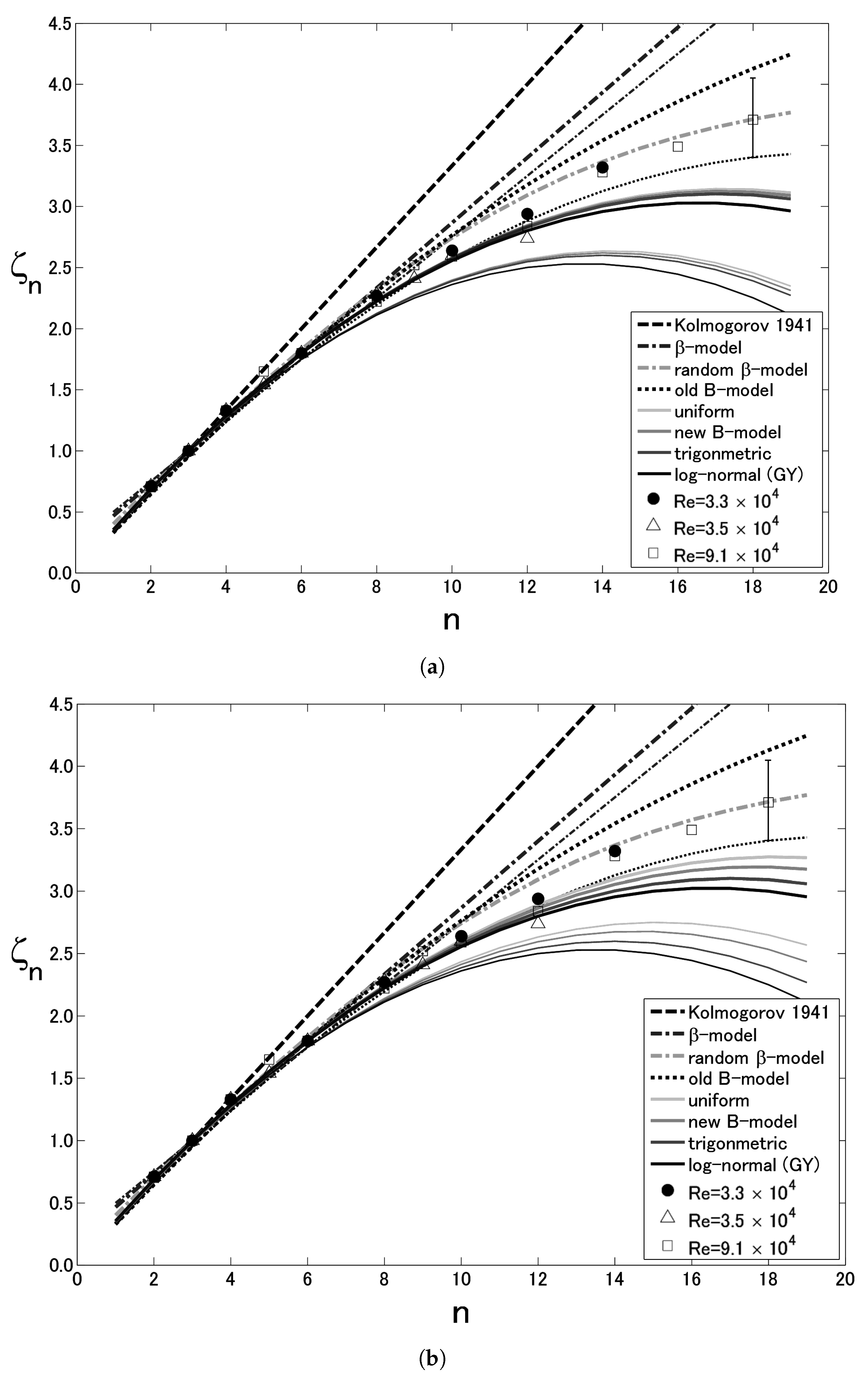
It was noted in Y90 that for the GY model and B-model are convex functions of n, so there is the pathological characteristic that eventually becomes negative at high orders, but that the B-model exhibits this tendency less than GY. When we extrapolated out the plots of in Figure 6, it can be seen that, while the B-model is less convex than GY, the difference between the two is much less pronounced than in Y90.
Similarly to the case of in Figure 5, when , the different pdfs tend to give similar curves, but when is increased to 5 the differences are enhanced. This dependence of the B-model on , the ratio of length scales, stresses a possible limitation of the model. In all cases, the curves are much lower and closer to GY than the B-model curves of Y90.
4.4. Range of and
One interesting question is the sensitivity of the model to the scale ratio . Y90 only considered because, as defined, the incorrect B-model equations were only solvable for . In this study, solutions exist all the way down to , and when is greater than 5 the changes are negligible. When was plotted for and compared with those of , the two cases were almost indistinguishable from each other.
The B-model of Y90 considered two possibilities for : 0.2 and 0.25. With the above changes, these two values of give less agreement with the empirical data of Anselmet et al. [15]. In order for the power law coefficient to agree with data, the intermittency coefficient could be as low as 0.17. Such lower curves are included in Figure 7 and are discussed in more detail next.
4.5. Model Comparisons
The original and revised versions of the B-model [6] belong to a family of discrete cascade models where , that includes the log-normal model [10], the -model [20], the random -model [21], and the -model and the p-model [22,23,24] (see also [16] for a review). However, discrete models are less realistic in a phenomenological sense, as they imply an elementary scale ratio (e.g., for the B-model) corresponding to discrete scales, whereas in turbulence intermittent fluctuations intrinsically exist at all scales. As such, continuous cascade models may provide a better alternative to study the stochastic properties of turbulent intermittent fluctuations. To our knowledge, three such models have been described in the literature: the log-Lévy model of Schertzer & Lovejoy [25], the log-Gamma model of Saito [18], and the log-Poisson model of Dubrulle [26], She & Leveque [19], and She & Waymire [27]. The corresponding formulations for the structure function exponents are given below:
1. Log-Lévy model:
is the codimension of the mean events (, where d is the dimension of the observation space, i.e., for a time-series), and is the Lévy index, bounded between 0 and 2. Specifically, the log-Lévy model is equivalent to the -model when and to the log-normal model when . The log-Lévy models can then be regarded as a family of models bounded between the -model and the log-normal model.
2. Log-Gamma model:
is a characteristic parameter of the gamma distribution (see e.g., [28]), and d is the dimension of the observation space.
3. Log-Poisson model:
is the codimension, which plays a similar role to of the log-Lévy model, but this parameter characterizes the extreme events. Another parameter, , is linked to the maximum singularity (i.e., the most extreme event) reachable from a finite sample. She & Leveque [19] proposed the general relation with and ,
which is in remarkable agreement with the experimental results of Benzi et al. [29].
The log-Lévy, log-Gamma, and log-Poisson models all provide very good fits to empirical data in both atmospheric and oceanic turbulence [16,30]. It is nevertheless stressed that, in contrast with the log-Lévy model, the log-Gamma and log-Poisson models have some limitations. First, the Gamma and Poisson distributions are not stable. In other words, a linear combination of Poisson variables does not follow a Poisson distribution [28], and hence the limitation of the multiplicative approach is clear from . Secondly, in the log-Poisson model, the values of the parameters c and are linked to the sample size of a given data set. The parameter is associated with the maximum singularity: the longer the available data set, the higher the probability of encountering new rare events, and thus, the higher the value of . Note that this directly affects the formulation of in Equation (51), and so implicitly limits its generality and fitting power. The same limitations apply to c insofar as this parameter describes the absolute distribution of rare events .
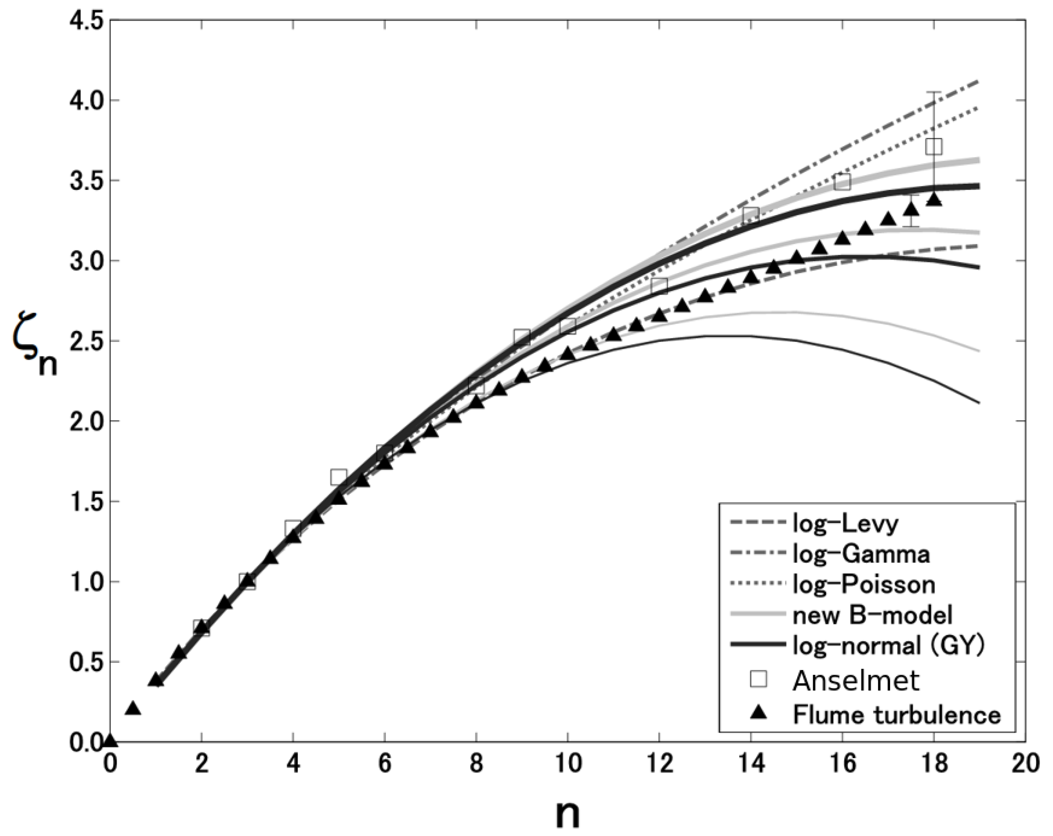
A comparison of these continuous cascade models to the B-model and the GY model are given in Figure 7. The values of the parameters used in Figure 7 for the continuous cascade models are and for log-Lévy (Seuront & Yamazaki, unpublished data), and taken from Saito [18] for log-Gamma and She & Leveque [19] for log-Poisson. An intermittency coefficient value of was also included in this figure, which shows good agreement with the data of [15] for very large values of n. This may suggest that the true is less than 0.2. However, significant differences between the fitting power of these models only start appearing for power exponents above 12th order. Hence, it is stressed that an unambiguous quantitative assessment of these models relies on large (i.e., typically with more than data points) experimental data sets with lower uncertainties and/or high quality.
To look at higher power exponents, we used large high quality data sets which have become available for in situ and ex situ with noticeable improvement in both the resolution and precision of turbulence measuring techniques such as shear sensors, particle imaging velocimetry and hot film and hot wire velocimetry. This has been illustrated using large data sets (ca. data points) of velocity fluctuations recorded in the laboratory via hot film velocimetry in a turbulent flume as discussed in Section 3. The corresponding exponents consistently converge to constant values up to 18th order and are shown in Figure 7. Note that, while , the slope of the order structure function, converges well, the moments themselves are much more sensitive, as recognized early on by [15]. This work only looks at the slope of the structure function though, so this difficulty is avoided, and the data presented here implies that is bounded between and . Nevertheless, future experiments with high quality data of the moments themselves for orders beyond 12 could go a long way in helping distinguish between different competing breakage models, including the B-model.
5. Conclusions
Two mistakes in the Y90 paper were identified and corrected, and the effects on the model of these corrections were discussed. We have tested the range of behaviours that the B-model can produce. Two new pdfs were introduced and an analogous analysis was carried out. It was found that, for and , these new pdfs gave behaviour with minor differences from the B-model and log-normal model. We also discussed the differences existing between the B-model, an example of a family of discrete cascade models, and the continuous cascade models available in the literature.
For the above values of the power exponent curves do not match up very well with the historical data of Anselmet et al. [15]. This data is not enough to completely distinguish between different values of data going past 12th order in structure function exponents. Beyond these relatively low Reynolds number data (i.e., Re between in a turbulent duct and below in a turbulent jet), structure function analysis has been proved to be a powerful tool to distinguish the fitting power of both discrete and continuous cascade models on highly turbulent atmospheric and oceanic turbulence data [16,30,31,32,33] for moments lower than 10th order. When a large data set (>) of high quality data is considered (Figure 7 and Section 3), the slope of the structure function can be estimated well to higher orders. Good agreement with the model is then found up to 18th order moments for between and . Future experiments that can probe not just the slope of the structure function, but the moments themselves too, would enable studies to better distinguish between the various breakage models.
Author Contributions
H.Y. conceived this study; C.L. found mistakes in Y90 manuscript [6] and developed new models; L.S. provided laboratory data set; C.L. prepared manuscript with input from H.Y. and L.S.
Funding
This work was partially supported by a grant (JPMJCR12A6) from Core Research for Evolution Science and Technology (CREST), a Japan Science and Technology Agency.
Conflicts of Interest
The authors declare no conflict of interest.
References
- Pope, S.B. Turbulent Flows; Cambridge University Press: Cambridge, UK, 2000. [Google Scholar]
- Menter, F.R. Two-equation eddy-viscosity turbulence models for engineering applications. AIAA J. 1994, 32, 1598–1605. [Google Scholar] [CrossRef] [Green Version]
- Speziale, C.G.; Sarkar, S.; Gatski, T.B. Modelling the pressure—Strain correlation of turbulence: An invariant dynamical systems approach. J. Fluid Mech. 1991, 227, 245–272. [Google Scholar] [CrossRef]
- Mishra, A.A.; Girimaji, S.S. Toward approximating non-local dynamics in single-point pressure–strain correlation closures. J. Fluid Mech. 2017, 811, 168–188. [Google Scholar] [CrossRef]
- Sagaut, P. Large Eddy Simulation for Incompressible Flows: An Introduction; Springer Science & Business Media: Berlin, Germany, 2006. [Google Scholar]
- Yamazaki, H. Breakage models: Lognormality and intermittency. J. Fluid Mech. 1990, 219, 181–193. [Google Scholar]
- Frisch, U. The Legacy of A. N. Kolmogorov; Cambridge University Press: Cambridge, UK, 1995. [Google Scholar]
- Kolmogorov, A.N. The local structure of turbulence in incompressible viscous fluid for very large Reynolds numbers. Doklady Akad. Nauk SSSR 1941, 30, 299–303. [Google Scholar] [CrossRef]
- Frisch, U. Fully developed turbulence and intermittency. Ann. N. Y. Acad. Sci. 1995, 357, 359–367. [Google Scholar] [CrossRef]
- Gurvich, A.S.; Yaglom, A.M. Breakdown of eddies and probability distributions for small scale turbulence. Phys. Fluids 1967, 10, 59–65. [Google Scholar] [CrossRef]
- Monin, A.S.; Ozmidov, R.V. Turbulence in the Ocean; Springer: Dordrecht, The Netherlands, 1985; p. 247. [Google Scholar]
- Kolmogorov, A.N. A refinement of previous hypotheses concerning the local structure of turbulence in a viscous incompressible fluid at high Reynolds number. J. Fluid Mech. 1962, 13, 82–85. [Google Scholar] [CrossRef]
- Gradshteyn, I.S.; Ryzhik, I.M. Table of Integrals, Series, and Products; Academic Press: Cambridge, MA, USA, 1980. [Google Scholar]
- Batchelor, G.K. The Theory of Homogeneous Turbulence; Cambridge University Press: Cambridge, UK, 1953. [Google Scholar]
- Anselmet, F.; Gagne, Y.; Hopfinger, E.J.; Antonia, R.A. High-order velocity structure functions in turbulent shear flows. J. Fluid Mech. 1984, 140, 63–89. [Google Scholar] [CrossRef]
- Seuront, L.; Yamazaki, H.; Schmitt, F. Intermittency (Chapter 7). In Marine Turbulence: Theories, Observations and Models; Cambridge University Press: Cambridge, UK, 2005; pp. 66–78. [Google Scholar]
- Tennekes, H.; Lumley, J.L. A First Course In Turbulence; MIT Press: Cambridge, MA, USA, 1972. [Google Scholar]
- Saito, Y. Log-gamma distribution model of intermittency in turbulence. J. Phys. Soc. Jpn. 1992, 61, 403–406. [Google Scholar]
- She, Z.-S.; Leveque, E. Universal scaling laws in fully developed turbulence. Phys. Rev. Lett. 1994, 72, 336–339. [Google Scholar]
- Frisch, U.; Sulem, P.-L.; Nelkin, M. A simple dynamical model of intermittent fully developed turbulence. J. Fluid Mech. 1978, 87, 719–736. [Google Scholar] [CrossRef]
- Benzi, R.; Paladin, G.; Parisi, G.; Vulpiani, A. On the multifractal nature of fully developed turbulence and chaotic systems. J. Phys. A 1984, 17, 3521–3531. [Google Scholar] [CrossRef] [Green Version]
- Schertzer, D.; Lovejoy, S. On the dimension of atmospheric motions. In Turbulence and Chaotic Phenomena in Fluids; Tatsumi, T., Ed.; Elsevier Science Ltd.: Amsterdam, The Netherlands, 1984; pp. 505–512. [Google Scholar]
- Schertzer, D.; Lovejoy, S. The Dimension and Intermittency of Atmosphereic Dynamics; Springer: Berlin/Heidelberg, Germany, 1985; pp. 7–33. [Google Scholar]
- Meneveau, C.; Sreenivasan, K.R. Simple multifractal cascade model for fully developed turbulence. Phys. Rev. Lett. 1987, 59, 1424–1427. [Google Scholar]
- Schertzer, D.; Lovejoy, S. Physical modeling and analysis of rain and clouds by anisotropic scaling multiplicative processes. J. Geophys. Res. 1987, 92, 9693–9714. [Google Scholar] [CrossRef]
- Dubrulle, B. Intermittency in fully developed turbulence: Log-Poisson statistics and generalized scale covariance. Phys. Rev. Lett. 1994, 73, 959–962. [Google Scholar] [CrossRef]
- She, Z.-S.; Waymire, E.C. Quantized energy cascade and log-Poisson statistics in fully developed turbulence. Phys. Rev. Lett. 1995, 74, 262–265. [Google Scholar] [CrossRef]
- Feller, W. An Introduction to Probability Theory and Its Applications; Wiley: New York, NY, USA, 1968; Volume 1. [Google Scholar]
- Benzi, R.; Ciliberto, S.; Baudet, C.; Ruiz Chavarria, G.; Tripiccione, R. Extended self-similarity in the dissipation range of fully developed turbulence. Europhys. Lett. 1993, 24, 275–279. [Google Scholar] [CrossRef]
- Yamazaki, H.; Mitchell, J.G.; Seuront, L.; Wolk, F.; Li, H. Phytoplankton microstructure in fully developed oceanic turbulence. Geophys. Res. Lett. 2006, 33, L01603. [Google Scholar] [CrossRef]
- Benzi, R.; Ciliberto, S.; Baudet, C.; Chavarria, G.R. On the scaling of three-dimensional homogeneous and isotropic turbulence. Phys. D Nonlinear Phenom. 1995, 80, 385–398. [Google Scholar] [CrossRef]
- Ruiz-Chavarria, G.; Baudet, C.; Ciliberto, S. Scaling laws and dissipation scale of a passive scalar in fully developed turbulence. Phys. D Nonlinear Phenom. 1996, 99, 369–380. [Google Scholar] [CrossRef]
- Schmitt, F.; Schertzer, D.; Lovejoy, S.; Brunet, Y. Multifractal temperature and flux of temperature variance in fully developed turbulence. Eur. Phys. Lett. 1996, 34, 195–200. [Google Scholar] [CrossRef]
Figure 1.
Schematic illustration of the flume experiment set up (see Section 3).
Figure 1.
Schematic illustration of the flume experiment set up (see Section 3).

Figure 2.
Power spectrum as a function of the wavenumber of data generated from flume experiment (normalized to be unitless, and displayed in log-scale). Dotted line is the slope.
Figure 2.
Power spectrum as a function of the wavenumber of data generated from flume experiment (normalized to be unitless, and displayed in log-scale). Dotted line is the slope.

Figure 3.
Illustration of the role of sample size in the convergence of the functions (top panel) and (bottom panel) as sample size N increases, for a sample size of .
Figure 3.
Illustration of the role of sample size in the convergence of the functions (top panel) and (bottom panel) as sample size N increases, for a sample size of .

Figure 4.
Pdf distributions for (a) and (b) corresponding to the case where .

Figure 5.
Correction factor for the universal spectrum slope with (a) , and (b) . The dotted line of the old B-model is done for in both cases. Gray-scale solid lines are listed in the legend in the order they appear in the figure from top to bottom.
Figure 5.
Correction factor for the universal spectrum slope with (a) , and (b) . The dotted line of the old B-model is done for in both cases. Gray-scale solid lines are listed in the legend in the order they appear in the figure from top to bottom.

Figure 6.
Power exponents of order structure function for (a) and (b) . In the cases where there are two lines of a given model (e.g., old B-model), the highest curve (thicker line) corresponds to ; the lowest (thinner line) to . The old B-model curves are done for in both plots. Grey-scale solid lines are listed in the legend in the order they appear in the figure from top to bottom. Experimental data points are compiled from Anselmet et al. [15] with the corresponding Reynolds number in the legend.

Figure 7.
Power exponents of order structure function for , including continuous cascade models. In the case of the B-model, and GY model where there are three lines each, the highest curve (thickest line) corresponds to ; the middle (moderate thickness), to ; the lowest (thinnest line), to . Parameters for the log-Lévy model are and (Seuront & Yamazaki, unpublished data) and are taken from Saito [18] for the log-Gamma, and She & Leveque [19] for the log-Poisson model. Experimental data points are from Anselmet et al. [15] for white boxes (Reynolds number of ), while the black triangles correspond to velocity fluctuations recorded in a circular flume using hot film velocimetry () (see [16] and Section 3). Error bars (only last shown for clarity) are standard deviations of the independent estimates from the flume experiment of Section 3.


Table 1.
Comparison of , , and for the four choices of pdf.
| Model | |||||
|---|---|---|---|---|---|
| B-model | −0.06250 | −0.07643 | −0.1352 | −0.1634 | |
| 0.1318 | 0.1631 | 0.2961 | 0.3645 | ||
| 0.0049 | 0.0074 | 0.0080 | 0.012 | ||
| Uniform pdf | −0.06124 | −0.07446 | −0.1243 | −0.1475 | |
| 0.1306 | 0.1611 | 0.2853 | 0.3488 | ||
| 0.0059 | 0.0088 | 0.011 | 0.017 | ||
| Trigonometric pdf | −0.06389 | −0.07848 | −0.1485 | −0.1824 | |
| 0.1332 | 0.1651 | 0.3094 | 0.3836 | ||
| 0.0039 | 0.0059 | 0.0039 | 0.0058 | ||
| Log-normal (GY) | −0.06930 | −0.08663 | −0.1609 | −0.2012 | |
| 0.1386 | 0.1733 | 0.3219 | 0.4024 | ||
| 0.000007 | 0.000007 | 0.000003 | 0.000002 | ||
© 2019 by the authors. Licensee MDPI, Basel, Switzerland. This article is an open access article distributed under the terms and conditions of the Creative Commons Attribution (CC BY) license (http://creativecommons.org/licenses/by/4.0/).
Share and Cite
MDPI and ACS Style
Locke, C.; Seuront, L.; Yamazaki, H. A Correction and Discussion on Log-Normal Intermittency B-Model. Fluids 2019, 4, 35. https://doi.org/10.3390/fluids4010035
AMA Style
Locke C, Seuront L, Yamazaki H. A Correction and Discussion on Log-Normal Intermittency B-Model. Fluids. 2019; 4(1):35. https://doi.org/10.3390/fluids4010035
Chicago/Turabian StyleLocke, Christopher, Laurent Seuront, and Hidekatsu Yamazaki. 2019. "A Correction and Discussion on Log-Normal Intermittency B-Model" Fluids 4, no. 1: 35. https://doi.org/10.3390/fluids4010035