Field Studies and 3D Modelling of Morphodynamics in a Meandering River Reach Dominated by Tides and Suspended Load

Abstract

Meandering is a common feature in natural alluvial streams. This study deals with alluvial behaviors of a meander reach subjected to both fresh-water flow and strong tides from the coast. Field measurements are carried out to obtain flow and sediment data. Approximately 95% of the sediment in the river is suspended load of silt and clay. The results indicate that, due to the tidal currents, the flow velocity and sediment concentration are always out of phase with each other. The cross-sectional asymmetry and bi-directional flow result in higher sediment concentration along inner banks than along outer banks of the main stream. For a given location, the near-bed concentration is 2−5 times the surface value. Based on Froude number, a sediment carrying capacity formula is derived for the flood and ebb tides. The tidal flow stirs the sediment and modifies its concentration and transport. A 3D hydrodynamic model of flow and suspended sediment transport is established to compute the flow patterns and morphology changes. Cross-sectional currents, bed shear stress and erosion-deposition patterns are discussed. The flow in cross-section exhibits significant stratification and even an opposite flow direction during the tidal rise and fall; the vertical velocity profile deviates from the logarithmic distribution. During the flow reversal between flood and ebb tides, sediment deposits, which is affected by slack-water durations. The bed deformation is dependent on the meander asymmetry and the interaction between the fresh water flow and tides. The flood tides are attributable to the deposition, while the ebb tides, together with run-offs, lead to slight erosion. The flood tides play a key role in the morphodynamic changes of the meander reach.

1. Introduction

Meandering is one of the most common shapes formed by river streams, which is especially true for streams in the lowland alluvial plains [1]. Due to meandering, the characteristics of water flow, sediment transport and the resulting bed deformation are more complex than in relatively straight river reaches. For a coastal river, the tidal currents interact with the fresh-water run-off and they form a bidirectional flow, which also plays an essential role in the fluvial process. This is especially true if the tides are much stronger than the fresh-water discharges. With a landward decline in strength, the tidal influence descends.

At the meander bend apex, its cross-sectional shape is usually asymmetrical, with a deep portion of channel along the outer bank and a broad, shallow section extending towards the inner bank. The plane curvature and cross-sectional asymmetry topography are shown to produce significant secondary currents and transverse water-surface slopes [2,3]. The secondary currents derive from the centrifugal acceleration acting on the stratification between the upper and lower flow layers.

It has also been proved that strong stratified currents have significant impacts on the distribution of bed shear stresses along the wetted perimeter of river, and thereby play an essential role in the sediment transport as well as morphology changes [3,4,5,6]. The bed changes induced by erosion and deposition affect the flow, which in turn influences the shear-stress distribution, sediment component and bed topography [7]. Therefore, the coupling of the stratified currents, sediment movement and bed-form changes makes up an interactive response that characterizes the meandering morphodynamics.

Given its scientific and practical significance, the dynamic process in a meandering river, among several other issues, has to date been the object of numerous theoretical and experimental studies [8,9,10,11]. These contribute to the understanding of the meandering phenomena. Recently, the use of an acoustic doppler current profiler (ADCP) has permitted direct estimations of Reynolds stress in tidal environment rivers [12]. Further research, especially of field measurements, that focuses on river curvature and cross-sectional asymmetry and deals with the interaction between river run-off and tidal currents [3], is necessary.

In recent years, many numerical simulations have been performed of tidal flow and sediment transport in meandering rivers. Instead of simplifications and assumptions in physical model tests, complex river geometries and boundaries are directly modelled. In a meander, its flow is three dimensional [13]. As compared with 2D depth-averaged models, an application of a 3D model generates, in terms of sediment transport, more reliable results [14].

For meandering rivers, most 3D models applied to simulations are based on the Reynolds-Averaged Navier-Stokes (RANS) equations assuming time-independent flow and isotropic turbulence [4,6]. A recent development is the application of large and detached eddy simulation (LES, DES) models to meandering flows [15,16]. LES aims to capture the time-dependent flow and resolves the large-scale anisotropy of turbulence. Limited by central processing unit (CPU) time and convergence, it is often used for issues with low Reynolds numbers and of limited domain dimensions [6]. In contrast, Delft3D (Version 4.04, Delft, The Netherlands) has the advantage of time-effective computations when applied to large-scale river and ocean simulations.

Meandering with large curvatures is a characteristic of many streams in low-land coastal regions. Changes in both river curvature and bed topography are interrelated, and their geometric shapes need to be considered when assessing the effects of channel configuration on flow and sediment transport. In a tidal environment, the river reach is affected by both run-off and tides, in which shifts between flood and ebb tides induce, with regard to flow patterns and sediment transport, more complexity. As a result, in terms of erosion and deposition, the alluvial process is different, an issue of concern for practical applications, especially if the river is in an urban development area.

The study focuses on a meandering reach of an alluvial river subjected to strong tidal currents (compared to much lower fresh-water discharges). Suspended load accounts for approximately 95% of the sediment in the river. Field measurements are performed to record the flow and sediment data and to map the river bathymetry at selected occasions. The field data help understand the sediment movement characteristics in both horizontal and vertical directions. A 3D suspended-load transport model is incorporated into a hydrodynamic model and computes the flow patterns and morphological changes. By means of the two approaches, the objective of the study is to provide insight into the interplay between fresh-water flows and tidal currents, to illustrate the circulatory patterns of suspended load transport during the tidal rising and falling, and to make predictions of the bed deformation associated with the meandering properties (curvature, cross-channel asymmetry, etc.). The results provide a reference for studies of tidal fluvial processes in similar situations.

The paper includes a study area description, field measurements of flow and sediment, field data analyses, mathematical formulation, model setup with calibration and validation, major flow features and morphological changes.

2. Study Area

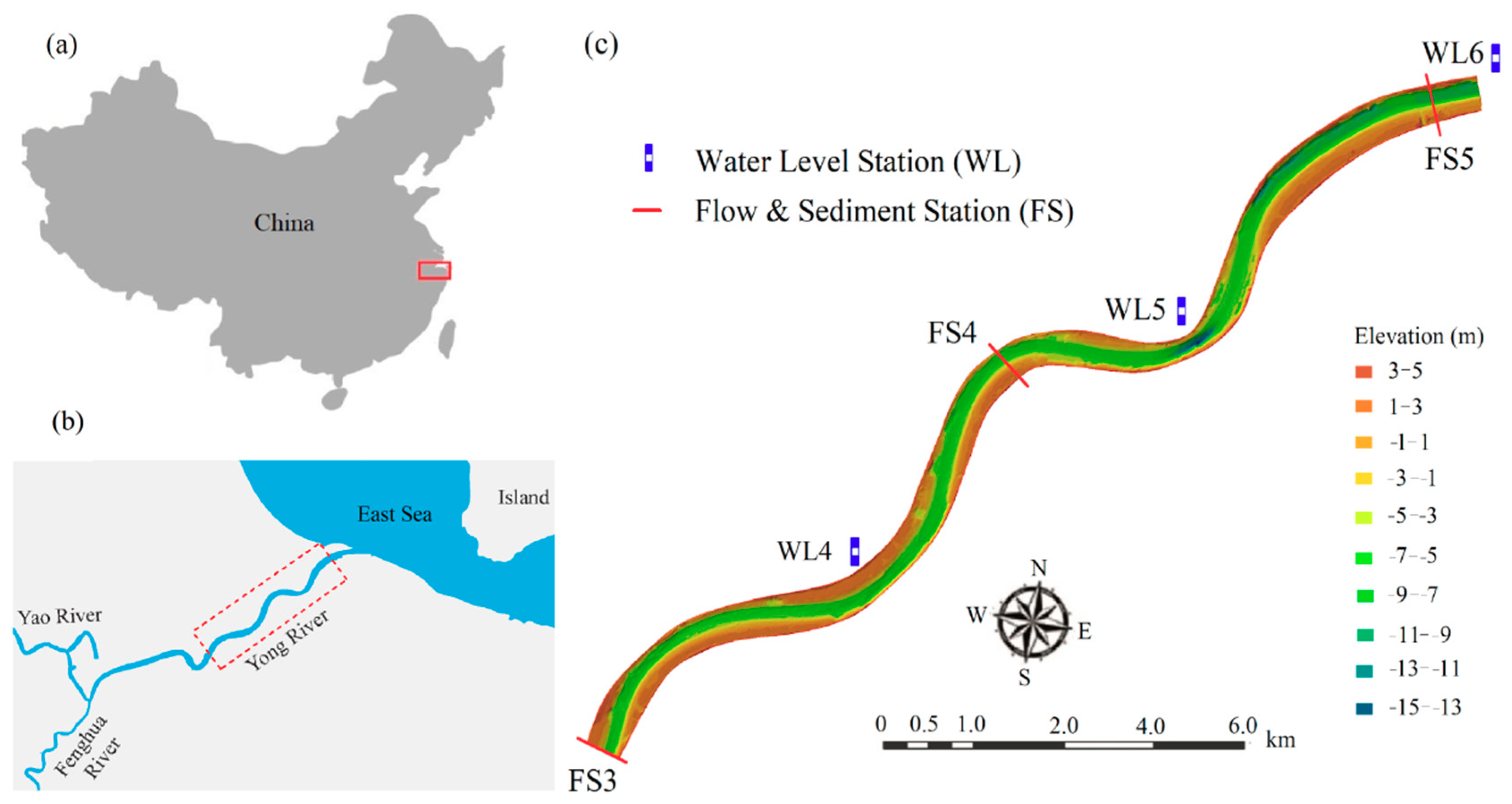
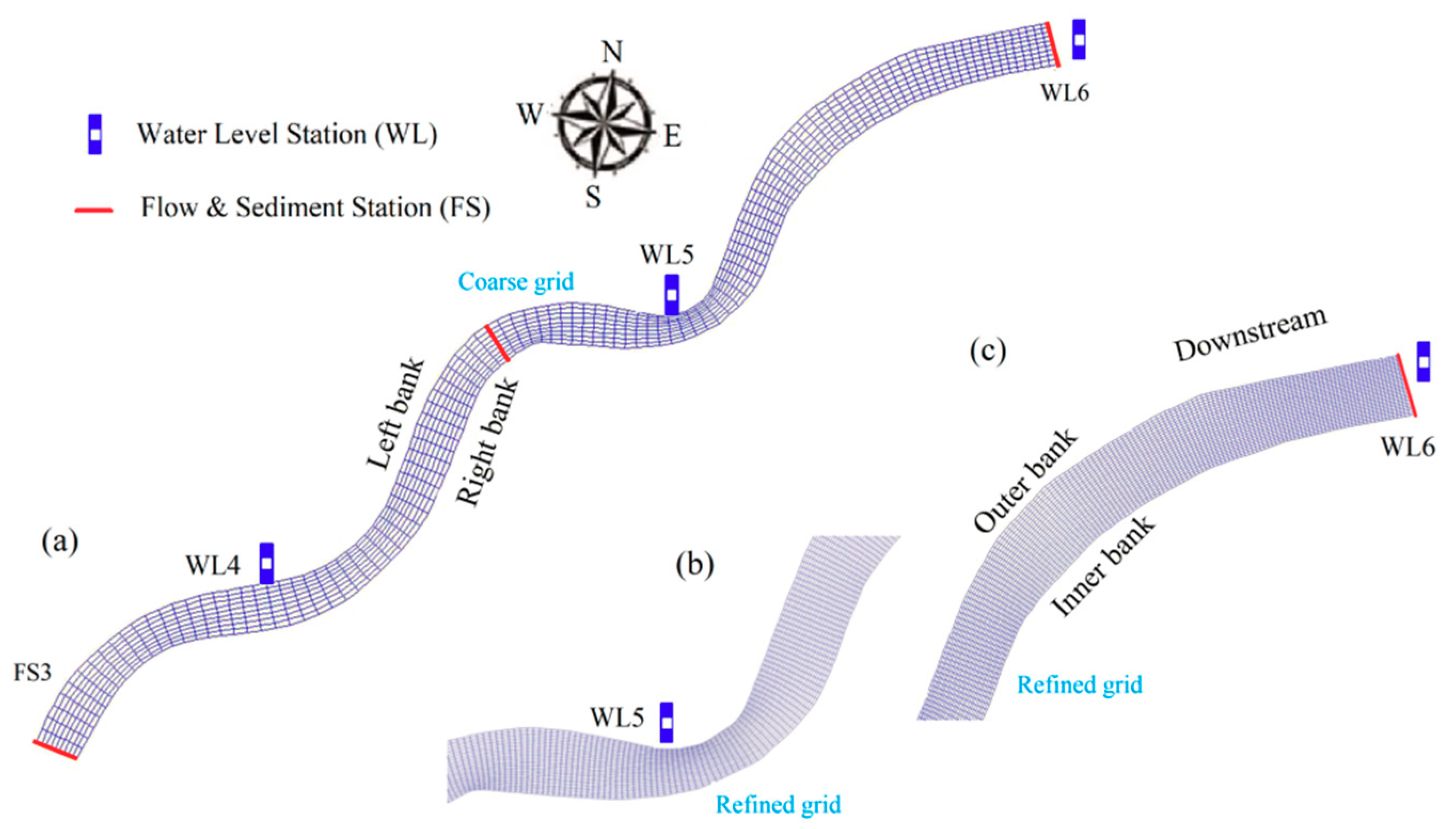
The study aims to examine an approximately sinusoidal meandering reach, with two successive, nearly S-shaped meander loops (Figure 1). The river runs into the sea and is subjected to strong tides.

The study area is part of the Yong River, located in Southeast China. The total area of the catchment is 42.94 km² (the area above the FS3 gauge is approximately 29 km). The river runs roughly in the SW–NE direction. The river length and width are about 26.5 km and 150–250 m measured on the normal water surface. The average river-bed slope is 1.17‰. The annual average rainfall is 1505 mm; the annual flow volume is 2.91 × 10⁹ m³; its annual average fresh-water discharge is 92 m³/s [17]. In a pronounced way, the flow and sediment transport in the river are affected by the tides from the coastal area. The annually averaged tidal flux is 946 m³/s, approximately 11 times the fresh-water flow discharge. The tides are the dominating factor for the sediment movement. Due to deposition, the river-bed rises, and the width narrows in many sections. This water system has been well managed since 1959, with regular dredging for navigation [18]. A single water course features the river mouth, without multiple branches, either at present or in the past.

The tide in the river is a semi-diurnal tide, i.e., two nearly equal high and low tides each day, belonging to the category of incomplete standing waves. According to the yearly statistics of hydrological stations, the average range of tidal levels is 0.29–0.44 m within one circle. The mean river depth is about 8 m, with tidal peak velocities close to 1 m/s; the tidal range increases landwards with the narrowing river width, with an average range falling between 1.62–1.84 m. During flood tides, sediment follows the currents and is transported from the outer sea area to the inland. This flow and sediment transport process reverse during ebb tides.

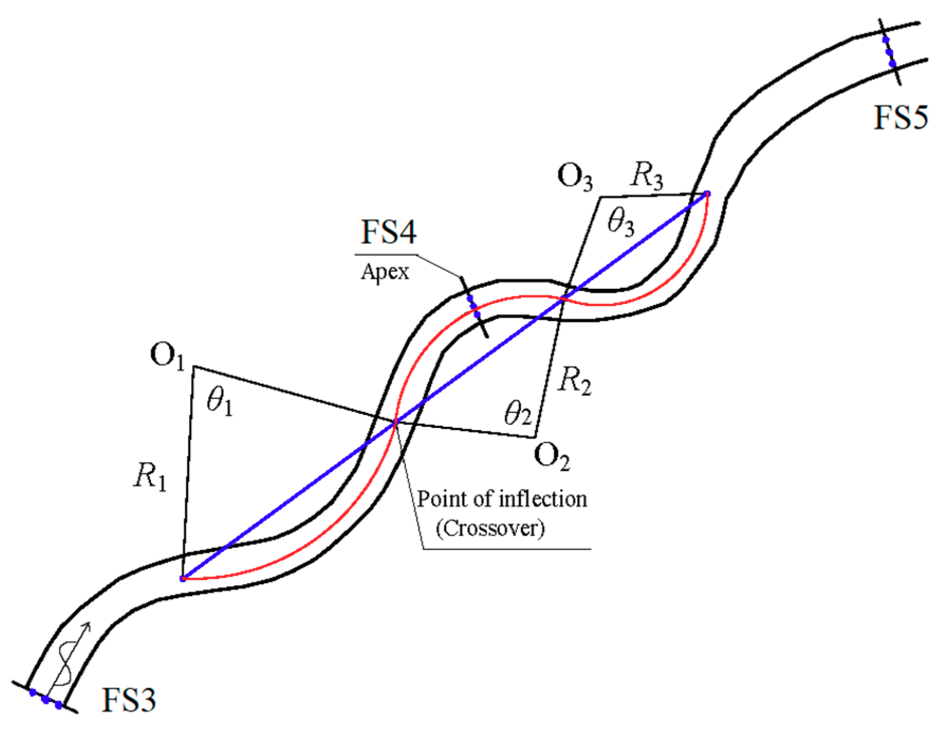
The meandering reach of interest has three consecutive parts of significant curvature (Figure 2). From up- to downstream, the radius of curvature is R ≈ 700, 500 and 300 m; their angles are θ ≈ 80°, 100° and 120°, respectively. The typical river width and water depth are about 200 m and 10 m. In addition, the meandering reach features large areas of shoals associated with high tidal levels, especially close to the apex positions. With these geometrical features, it is a typical site to understand the cross-sectional currents and asymmetric bed forms and their effects on sediment movement along the reach.

Further upstream of the study area, a confluence exists, where the Yao and Fenghua Rivers merge into the Yong River (Figure 1). Its sedimentation pattern, associated with different flow regimes, is also an issue of concern [19].

3. Field Measurements

3.1. Data Collection

To record the hydrological data and map the river bathymetry, extensive field surveys were carried out for the study area during the period June 2015–January 2016. The hydrological data used were acquired for a typical wet season in June 2015. The collected parameters included water levels, water-flow velocity, flow discharge, sediment concentration and grain-size distributions. The river bathymetry used for the study was achieved using an HY1600 bathymetric profiler.

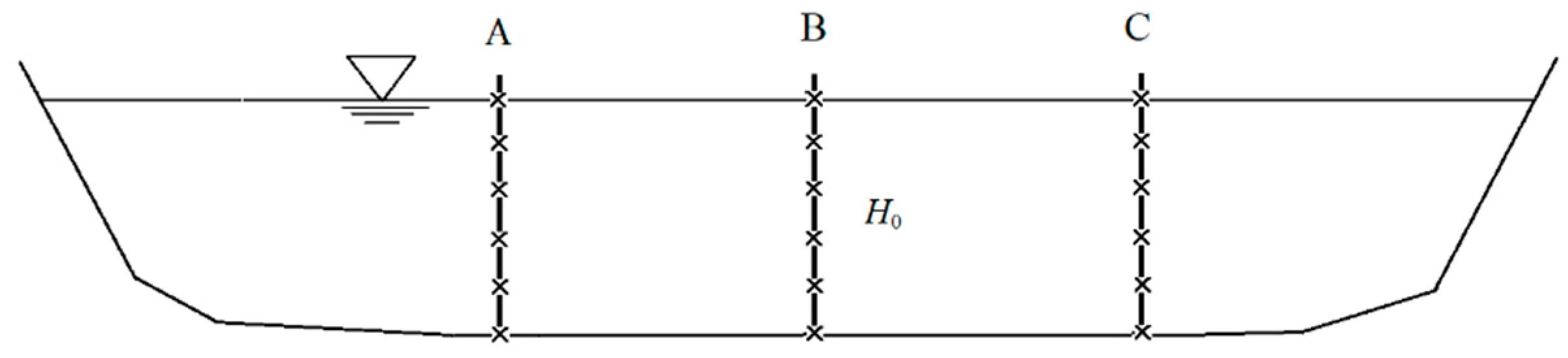
Also marked in Figure 1 are the recording stations for water levels (WL), at three locations (denoted as WL4, WL5 and WL6), and for flow & sediment (FS), also at three locations (denoted as FS3, FS4 and FS5). At each FS, three typical plumb lines (A, B and C, from left to right, looking downstream) were arranged (Figure 3). Along each line, sampling was made at six points, i.e., h_i = 0, 20%, 40%, 60%, 80% and 100% of the water depth H₀ (i = 1, 2, …, 6). All the data were recorded in a one-hour interval.

Four­beam 600/1200-kHz RDI Workhorse Acoustic Doppler Current Profilers (ADCPs) (Nortek group, Rud, Norway), measured flow velocities. Each ADCP was attached to its measurement vessel. The inaccuracy of the resulting flow discharges was below ±5%. The YJD-1 type pressure sensors (Tekscan, Inc., South Boston, MA, USA) were used for water-level measurements, with an inaccuracy of ±1 cm. Efforts were made on sampling of the suspended load, using point-integrative water samplers (Hoskin Scientific, Ltd., Saint-Laurent, QC, Canada). Samples of bed load, though small in amount, were also taken with Shipek grab samplers (Envco, Auckland, New Zealand) and their percentages were calculated.

The grain-size distribution of the suspended load was analyzed using an automatic sieving device (SFY-D) (Zhonghu Scientific Ltd., Nanjing, China) and an automated Laser particle-size analyzer (Mastersizer2000) (Malvern Panalytical Ltd., Malvern, UK). Particle sizes falling between the range 0.0002 and 2 mm were identified. The obtained data are well suited for calibration and validation of numerical models. The field data acquired for the wet season, including one spring and one neap tide, in June 2015 were used in the study.

For each WL and FS station, the time-series of the raw hydrological data were analyzed. For each time period, the average value of the FS sampling was first obtained for each line with the six points. Based on the three lines, cross-sectionally averaged sediment concentration, S (kg/m³), and flow velocity, V (m/s), were then achieved by the weighted average method given below:

$$S=\frac{{{\displaystyle \sum }}_i{S}_i{V}_i{h}_i}{{{\displaystyle \sum }}_i{V}_i{h}_i}$$

(1)

$$V=\frac{{{\displaystyle \sum }}_i{V}_i{h}_i}{{{\displaystyle \sum }}_i{h}_i}$$

(2)

where S_i and V_i = sediment concentration and velocity of each measured points, respectively.

3.2. Suspended versus Bed Load

Based on grain-size distribution, river sediment is classified as sand (0.05–2 mm), silt (0.005–0.05 mm) and clay (<0.005 mm) [20]. The field measurements show that suspended load consists of cohesive silt and clay and accounts for approximately 95% of the sediment.

Table 1. D₅₀ of suspended and bedload during the wet season (2nd half of June 2015).

Station	Spring Tide, D50 (mm)		Neap Tide, D50 (mm)
	Suspended Load	Bed Load	Suspended Load	Bed Load
FS3	0.007	0.011	0.008	0.012
FS4	0.008	0.019	0.006	0.020
FS5	0.008	0.011	0.007	0.011

shows their median grain sizes (D₅₀), which differ during spring and neap tides. For the former, the D₅₀ values vary between 0.007–0.008 mm for the suspended load and between 0.011–0.019 mm for the bed load. For the latter, the corresponding ranges are 0.006–0.008 mm and 0.011–0.020 mm.

3.3. Cross-Sectional Difference in Sediment Concentration

The second half of June 2015 includes 30 semi-diurnal tides, with 30 flood and ebb tides, respectively. To reveal the spatial changes of S at FS3, FS4 and FS5,

Table 2. Time-averaged S values during the wet season (2nd half of June 2015).

Station	Spring Tide (kg/m3)			Neap Tide (kg/m3)
	Flood Tide	Ebb Tide	Average	Flood Tide	Ebb Tide	Average
FS3	1.247	1.615	1.441	0.200	0.215	0.208
FS4	2.341	2.117	2.207	0.232	0.318	0.282
FS5	1.673	1.476	1.578	0.314	0.214	0.265

summarizes their time-averaged S values, with the following observations.

(1)

Going upstream from the river mouth, the S value is largest at FS4, with S = 2.341 kg/m³ during the spring tide.

(2)

At the same location for either the spring or neap tide, S during the flood tides differs from that during the ebb ones. The spring tides feature much higher values than the neap ones. This implies that the spring tides govern the sediment transport from the coastal area.

(3)

At the same location, S during the spring tide is 6−8 times as high as during the neap tide.

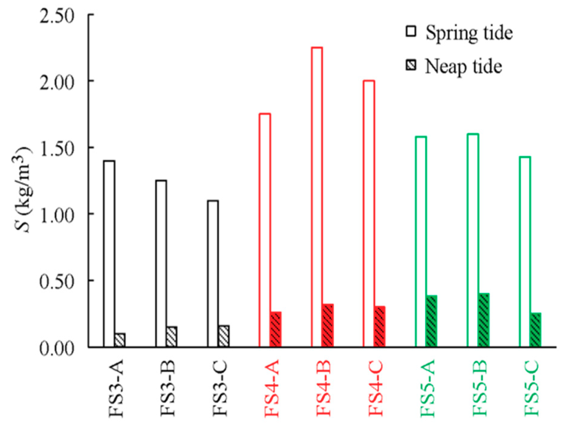
In a meander bend, the cross-sectional asymmetry affects the re-distribution of S, which in turn aggravates its asymmetry. For lines A, B and C at FS3, FS4 and FS5, Figure 4 displays, during the spring and neap tides, its distribution.

The following features are evident.

(1)

For each line, the spring-tide S value is significantly larger than the neap-tide one. This further indicates the former dominates the sediment transport from the coastal area.

(2)

At FS4, line A is nearest to the outer bank. In the spring tide, FS4-B exhibits the largest S value, followed by FS4-C and FS4-A. This shows that, around this bend apex, the water along the inner bank carries more sediment than along the outer bank. This is mainly ascribable to the asymmetry in cross-channel shape.

(3)

During the neap tide, the S values are much lower and are close at the same cross-section.

3.4. Vertical Difference in Sediment Concentration

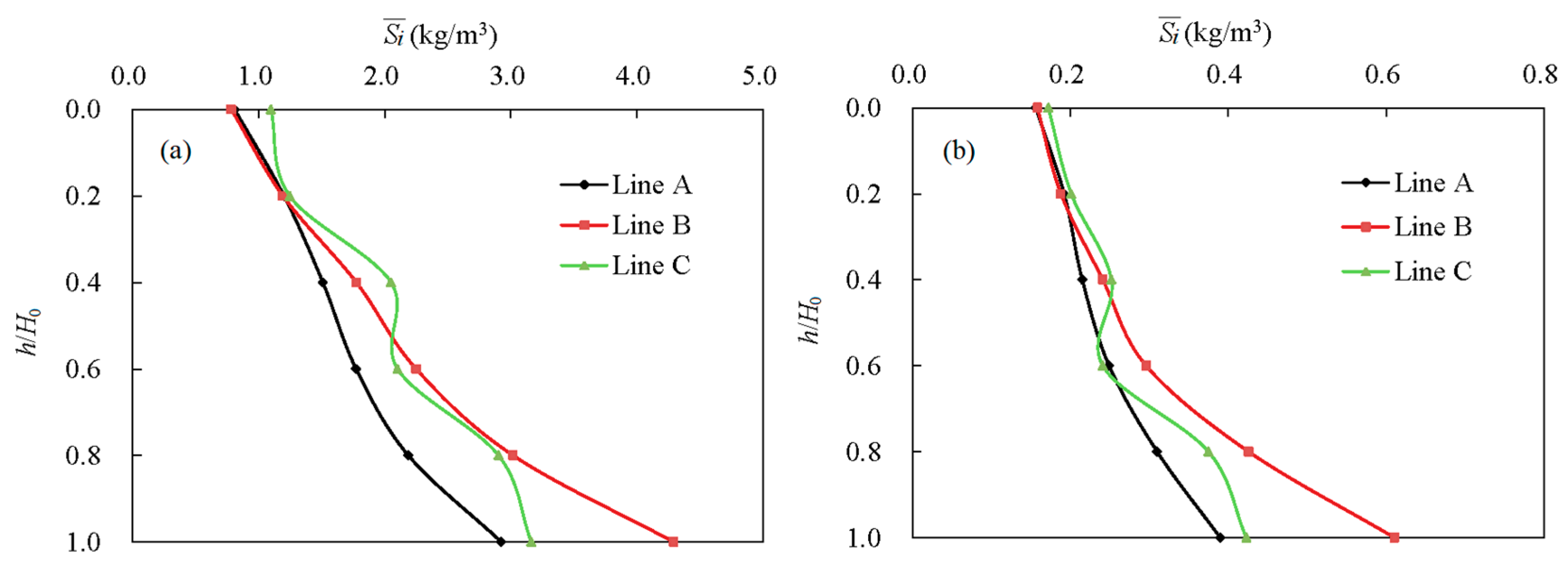
To look at the sediment distribution in the vertical direction, the measured results are analyzed along lines A, B, C at each FS location.

Table 3. Time-averaged sediment concentration ($\overline{S_i}$) along lines A, B and C during the wet season (2nd half of June 2015).

Vertical Line	Spring Tide (kg/m3)						Neap Tide (kg/m3)
	0	0.2H0	0.4H0	0.6H0	0.8H0	H0	0	0.2H0	0.4H0	0.6H0	0.8H0	1.0H0
FS3-A	0.872	-	-	1.412	-	1.798	0.139	0.148	0.160	0.170	0.181	0.241
FS3-B	0.643	0.871	1.062	1.233	1.581	1.996	0.157	0.177	0.191	0.202	0.214	0.279
FS3-C	0.633	0.786	0.941	1.151	1.320	1.761	0.189	0.206	0.216	0.226	0.239	0.273
FS4-A	0.809	1.201	1.509	1.773	2.187	2.925	0.156	0.192	0.215	0.249	0.310	0.390
FS4-B	0.783	1.193	1.775	2.249	3.018	4.292	0.158	0.188	0.241	0.296	0.426	0.611
FS4-C	1.097	1.246	2.050	1.902	2.903	2.962	0.172	0.201	0.252	0.241	0.375	0.423
FS5-A	0.876	1.135	1.443	1.739	1.989	2.349	0.133	0.174	0.278	0.343	0.493	0.600
FS5-B	0.906	1.200	1.490	1.717	1.982	2.409	0.119	0.146	0.246	0.348	0.483	0.747
FS5-C	0.564	-	-	1.547	-	2.048	0.061	-	-	0.202	-	0.385

shows, for each line, the time-averaged sediment concentration (denoted as $\overline{S_i}$) at h = 0, 0.2H₀, 0.4H₀, 0.6H₀, 0.8H₀ and H₀. As a showcase, Figure 5 illustrates, at FS4, its distribution along the lines.

The following patterns are observed:

(1)

The $\overline{S_i}$ distribution from the water surface to the river bed exhibits an increasing tendency. Close to the bed, the $\overline{S_i}$ value reaches a maximum. The value close to the bed is 2−5 times that close to the surface.

(2)

For a given line, the $\overline{S_i}$ values at h = 0.6H₀ are approximately equal to the line-averaged value.

(3)

At the same cross-section, the averaged $\overline{S_i}$ values along the B line are the largest. This implies that the main-channel flow carries most sediment.

(4)

For the same point, the $\overline{S_i}$ value during the spring tide is 3−7 times during the neap tide. This means that much more sediment is transported by the spring tide, which is a potential source of sedimentation in the area. The observations are consistent with the findings by Chen et al. [17] and Shen [18].

3.5. Tidal Effects

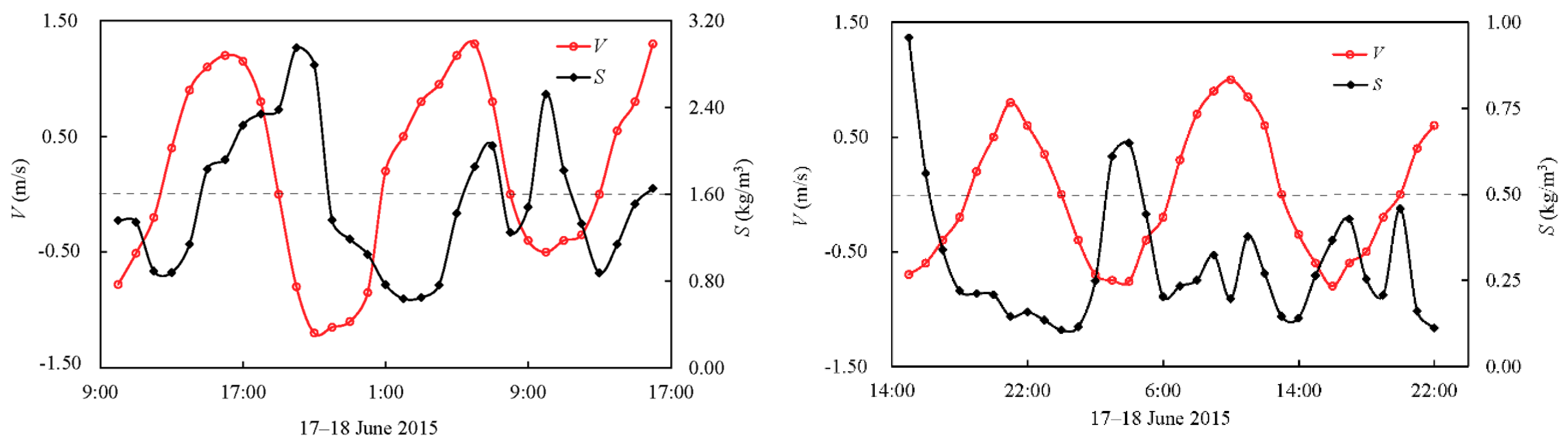
To further unveil the time dependence of sediment transport, Figure 6 illustrates, for the spring and neap tides, the relationship between S and V at cross-section FS5 (close to the river mouth). A positive V value indicates flow towards the sea and a negative V implies a reversal of the current. The FS3 and FS4 results are shown later in the numerical part.

At the river mouth, the V and S values in the spring tide are larger than in the neap tide. S varies greatly during a tidal period, with two peaks, implying that the tides govern the sediment concentration. The flood tidal V and S are always out of phase with each other; the S peak appears during the flood tides. The S is modified by the tides and other oceanic processes.

The spring tide dominates the river flow and transports the sediment in the river. The neap tide being relatively weak, the run-off plays a dominant role. As a result, S and V exhibit non-similarity between the spring and neap tides. The tides stir sediment, affects its peak duration and transport. Without the tides, sediment would be diverted directly downstream [21].

4. Numerical Modeling

3D numerical modeling of flow and sediment is performed for the tidal reach and it considers the following typical aspects: (1) bidirectional flow environment under the interaction between river run-off and tides; (2) spatial variations of roughness and bed asymmetry topography; (3) submergence and exposure of shoals due to tidal rising and falling; (4) stratified currents in meanders; and (5) graded suspended load.

4.1. Mathematical Formulation

The Delft3D 4.04 package [22] is used to examine the complex flow features and morphology changes. It is based on the finite-difference method and solves the Navier-Stokes equations. To simulate river-bed changes, it is necessary to supplement such control conditions as bed stability coefficient and riverbed resistance. Therefore, the governing equations include equations for flow continuity, flow momentum, sediment transport and the bed deformation.

The flow continuity equation is

$$\frac{\partial \mathsf{\zeta }}{\partial t}+\frac{\partial \left(H{U}_x\right)}{\partial x}+\frac{\partial \left(H{U}_y\right)}{\partial y}=q$$

(3)

where U_x (m/s) and U_y (m/s) = depth-averaged velocities in the x and y coordinate system, ζ (m) is the tidal level, d (m) is the still water depth, H (m) is the total water depth (H = ζ + d), q (m/s) is the global source or sink term per unit area and t (s) is time. The momentum equations in the x and y directions are

$$\frac{\partial u}{\partial t}+u\frac{\partial u}{\partial x}+v\frac{\partial u}{\partial y}+\frac{\omega }{H}\frac{\partial u}{\partial \sigma }-fv=-\frac{1}{{\rho }_0}{P}_u+F_u+\frac{1}{H^2}\frac{\partial }{\partial \sigma }\left(v_v\frac{\partial u}{\partial \sigma }\right)$$

(4)

$$\frac{\partial v}{\partial t}+u\frac{\partial v}{\partial x}+v\frac{\partial v}{\partial y}+\frac{\omega }{H}\frac{\partial v}{\partial \sigma }+fu=-\frac{1}{{\rho }_0}{P}_v+F_v+\frac{1}{H^2}\frac{\partial }{\partial \sigma }\left(v_v\frac{\partial v}{\partial \sigma }\right)$$

(5)

where ρ₀ (kg/m³) = water density, $v_v$ (m²/s) = vertical eddy viscosity, $P_u$ and $P_v$ (kg/(m²s²)) = pressure gradients, $F_u$ and $F_v$ (m/s²) = horizontal Reynolds stresses, f (1/s) = Coriolis parameter (inertial frequency) and u and v (m/s) = longitudinal and transversal velocity components. The vertical velocity ω (m/s) component is computed from the mass balance:

$$\frac{\partial \omega }{\partial \sigma }=-\frac{\partial \mathsf{\zeta }}{\partial t}-\frac{\partial \left(Hu\right)}{\partial x}-\frac{\partial \left(Hv\right)}{\partial y}+H\left(q_{\mathrm{in}}-q_{\mathrm{out}}+P-E\right)$$

(6)

where q_in and q_out (m/s) = local source and sink per unit volume, P (m/s) = precipitation and E (m/s) = evaporation.

As seen from the field data, the bed-load amount is comparatively small (below 5%). To simplify, only the cohesive suspended sediment is considered in the sediment transport model. For mass balance and advection-diffusion, the equation in 3D reads as

$$\frac{\partial S}{\partial t}+\frac{\partial }{\partial x}\left(us\right)+\frac{\partial }{\partial y}\left(vs\right)+\frac{\partial }{\partial \sigma }\left[\left(\omega -{\omega }_s\right)s\right]-\frac{\partial }{\partial x}\left({\epsilon }_{s,x}\frac{\partial S}{\partial x}\right)-\frac{\partial }{\partial y}\left({\epsilon }_{s,y}\frac{\partial S}{\partial y}\right)-\frac{\partial }{\partial \sigma }\left({\epsilon }_{s,z}\frac{\partial S}{\partial \sigma }\right)=- F_s$$

(7)

where ω_s (m/s) = sediment settling velocity, ε_s,x, ε_s,y and ε_s,z (m²/s) = eddy diffusivity of sediment fraction in three directions and F_s = function of the river-bed deformation, which is dependent on sediment erosion and deposition and is proposed as follows by Partheniades-Krone [23].

$${\gamma }_0\frac{\partial Z_b}{\partial t}=F_s$$

(8)

$$F_s=D_b-E_b$$

(9)

$$D_b=\{\begin{array}{cc}{\omega }_s{S}_b\left(1-\frac{\tau }{{\tau }_d}\right)& \tau \le {\tau }_d\\ 0& {\tau }_d<\tau \end{array}$$

(10)

$$E_b=\{\begin{array}{cc}M\left(\frac{\tau }{{\tau }_e}-1\right)& \tau \ge {\tau }_e\\ 0& \tau <{\tau }_e\end{array}$$

(11)

where Z_b (m) = change in bed elevation, γ₀ (N/m) = dry weight of bed load, D_b (kg/(m²s)) = sediment flux of deposition from suspended load, E_b (kg/(m²s)) = sediment flux of erosion resulting in suspended load, S_b (kg/m³) = bottom sediment concentration, τ (N/m²) = bed shear stress, τ_d and τ_e (N/m²) = critical stresses of deposition and erosion and M (kg/m²s) = bed scouring rate.

4.2. Grid and Bathymetry

The river reach of interest is composed of three consecutive bends. The bathymetry is based on the measured topography data in June 2015 (Figure 1c). The computational domain is 13.2 km long and includes 1000 m upstream and 1200 m downstream to reduce boundary effects. Several grids of varied cell sizes are evaluated to ensure grid independence. Grid independence is checked through steady-state calculations. Based on a coarse mesh (Figure 7a), both global and local refinements are made to achieve a finer mesh. Figure 7b,c show the local refinements of two sections.

After refinement, the domain is covered by 10 500 cells, comprising 350 streamwise cells and 30 transverse cells. Grid size varies between 10 and 20 m, a typical range for most river simulations [7,13,22]. Denser cells, with a minimum cell size of 5 m, are given to the outer bank to account for large flow velocity gradients. As recommended by the Deltares systems [22], 10 layers are specified in the vertical direction, with a thickness of 2%, 3%, 4%, 6%, 8%, 10%, 12%, 15%, 20% and 20% of H. The difference between two neighboring layers should not exceed the lower layer’s thickness.

4.3. Boundary Conditions

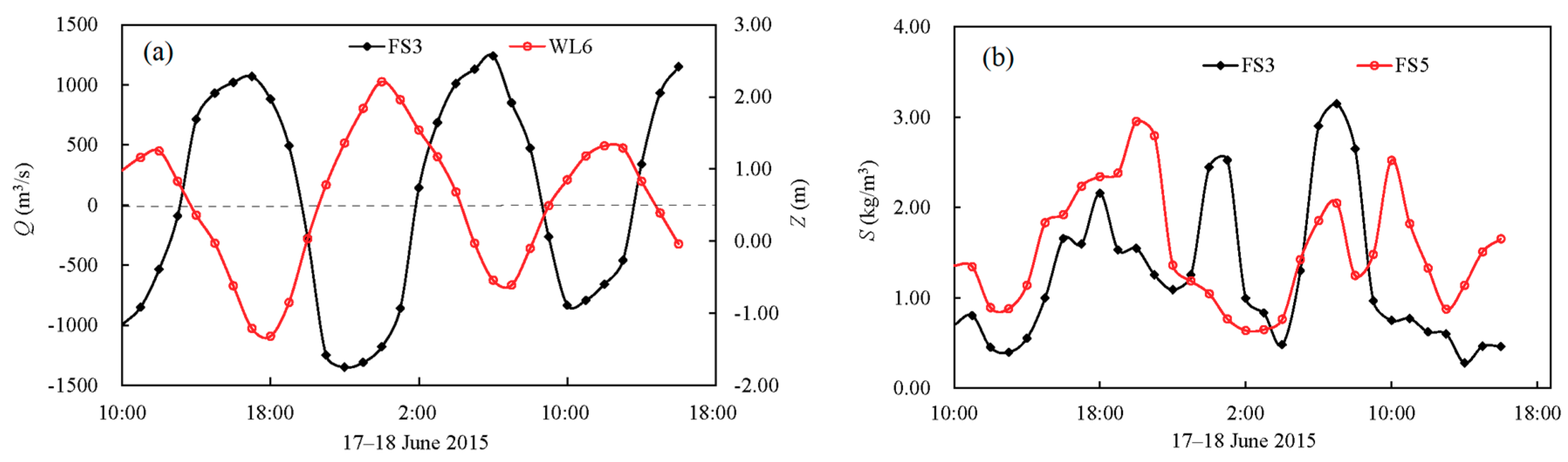
For flow computations, time-series of boundary conditions are specified with discharge, Q (m³/s), at the upstream end (FS3) and with water level, Z (m), at the downstream end (WL6) (Figure 8a). The time series of sediment concentration needs also be specified at both ends (Figure 8b). For the closed sediment boundary (river bed and banks), a non-entry condition specifies a zero normal gradient of sediment content. The wetting and drying function of cells is activated to account for the tidal rise and fall.

River-bed roughness, represented by Manning’s roughness equation, is an essential parameter dependent on such factors as river-bed morphology, flow patterns including water depth, etc. The range of Manning’s roughness falls within n = 0.015 to 0.030 m^−1/3 s, with 0.015–0.018 m^−1/3 s for the main channel and 0.018–0.030 m^−1/3 s for the shore beach, which is based on field investigations. For a given position, interpolation is made in light of water depth.

Table 4. Parameter values adopted in the model.

Parameter	Data Range	Source
${\omega }_s$ (m/s)	0.0005	Field measurements
${\tau }_d$ (N/m2)	0.06–0.10	Equation (10) [23]
${\tau }_e$ (N/m2)	0.10–0.20	Equation (11) [24]
M (kg/m2s)	0.0002–0.02	Equation (11) [24]
${\gamma }_0$ (kg/m3)	1600	Field measurements

summarizes the additional parameters, ω_s, τ_d, τ_e, M and γ₀, in the model setup.

To achieve numerical stability, the chosen time step is 0.3 s. For each time step, the flow is first calculated and the sediment transport and the resulting bed-level change are updated accordingly.

5. Model Calibration and Validation

Calibration, as well as validation, is a prerequisite for modelling accuracy. By adjusting specific parameters, a reasonable match is achieved between observed and simulated results. In the study, varying roughness coefficient in space, time step and open boundary conditions and refining the mesh are the tuning aspects. As in many other studies, the results turn out to be most sensitive to the roughness. Time steps (dependent on the grid density) and boundary conditions also have an influence on the model convergence; the grid density has a bearing on the accuracy of the results.

As shown in

Table 5. Error parameters and accepted ranges for model evaluation [25,26,27].

Parameter	Range	Optimal value	Satisfactory if	Expression
NSE	−∞–1	1	> 0.5	$E=1-\frac{{{\displaystyle \sum }}_{i=1}^n{\left(O_i-P_i\right)}^2}{{{\displaystyle \sum }}_{i=1}^n{\left(O_i-\overline{O}\right)}^2}$
R2	0–1	1	> 0.5	$R^2={\left(\frac{{{\displaystyle \sum }}_{i=1}^n\left(O_i-\overline{O}\right)\left(P_i-\overline{P}\right)}{\sqrt{{{\displaystyle \sum }}_{i=1}^n{\left(O_i-\overline{O}\right)}^2}\sqrt{{{\displaystyle \sum }}_{i=1}^n{\left(P_i-\overline{P}\right)}^2}}\right)}^2$
PBIAS	−∞–+∞	0	±25% for streamflow ±55% for sediment	$PBIAS= \frac{{{\displaystyle \sum }}_{i=1}^n\left(O_i-P_i\right)\times 100}{{{\displaystyle \sum }}_{i=1}^n{O}_i}$

, three model criteria, i.e., Nash-Sutcliffe efficiency (NSE), R-Squared (R²) and Percent bias (PBIAS) are often used for model evaluation, where $O_i$ = observed (in situ) value, $\overline{O}$ = average of $O_i$, $P_i$ = predicted value, $\overline{P}$ = average of $P_i$ and n = total number of observed or predicted values.

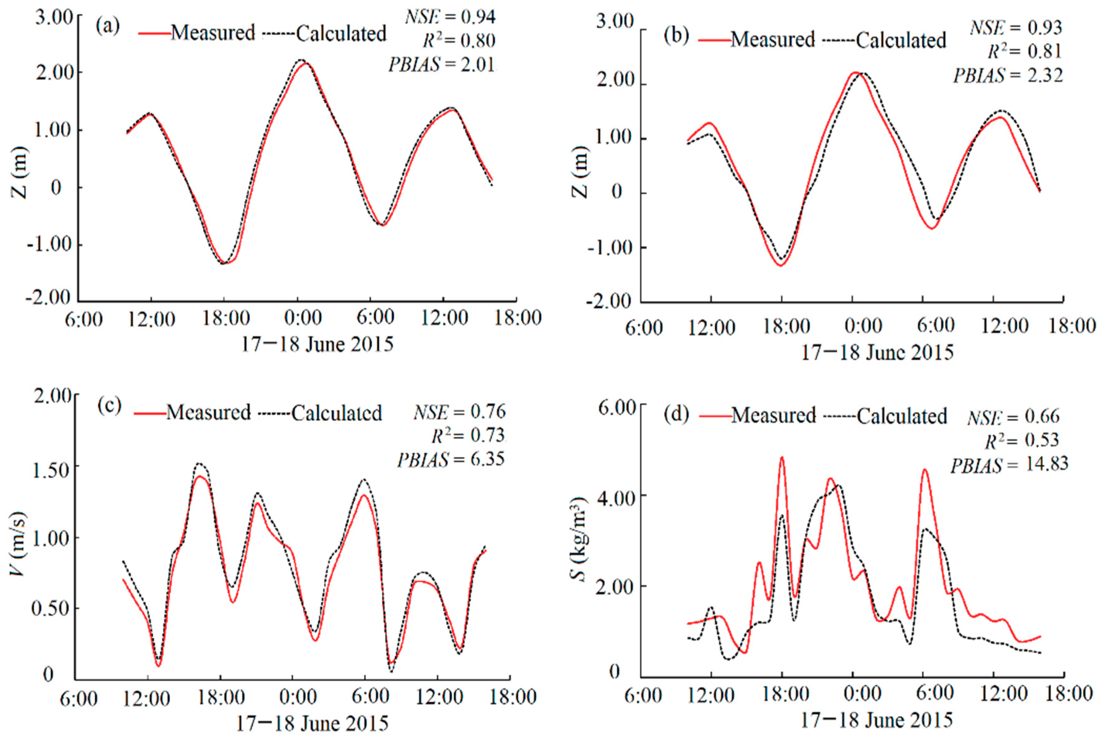
The model calibration is based upon the hourly data observed for the spring tide occurring between the period from 10:00 2015-06-17 to 16:00 2015-06-18; totally 30 h. Comparisons of water levels at WL4 and WL5 and of V and S at FS4 are shown in Figure 9.

The calibration results show that the calculated Z and V are in good agreement with the measured ones. All their error parameters meet the criteria. For S, the calculated and simulated results do not exhibit the exactly same pattern. However, the sediment peaks are, in terms of phase and magnitude, reasonably reproduced.

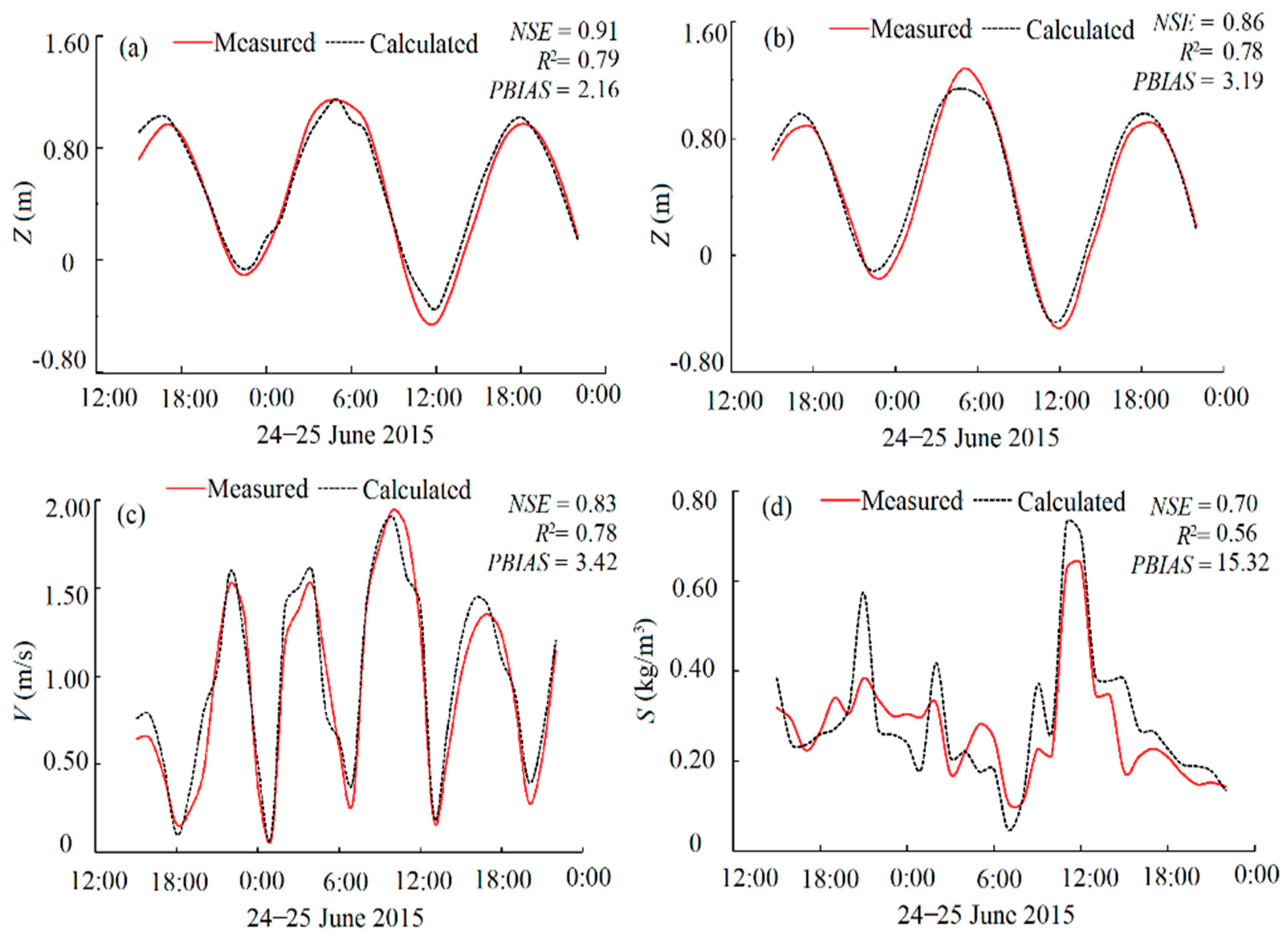
The model validation is performed with a neap tide that occurred during the period between 15:00 2015-06-24 and 22:00 2015-06-25, lasting a total of 31 h. It follows the same principle as model calibration. The validation results are shown in Figure 10.

The calculated Z, V and S profiles match relatively well with the measured data series. All the error parameter values also meet the requirements. As in other numerical simulations, the match between the measured and simulated parameters is better for Z and V than for S. The interplay between fresh-water flows and tides accounts for the difference in peak sediment concentration. The model generates acceptable results and it is suitable for prediction of flow and morphology changes of the meandering river reach.

6. Typical Flow Features

In the meandering reach, the flow features are of significant variations with stratified currents, in which cross-sectional velocity distributions often deviate from the logarithmic profile typical of straight reaches. Meanwhile, the bi-directional currents induced by flood and ebb tides also make the flow patterns more complex. A 2D depth-averaged model, with the assumption of a logarithmic velocity structure, would lead to inaccurate prediction in terms of, e.g., bed shear stress [22]. A 3D model is, therefore, necessary for prediction of such a tidal meander reach.

6.1. Cross-Sectional Flow Patterns

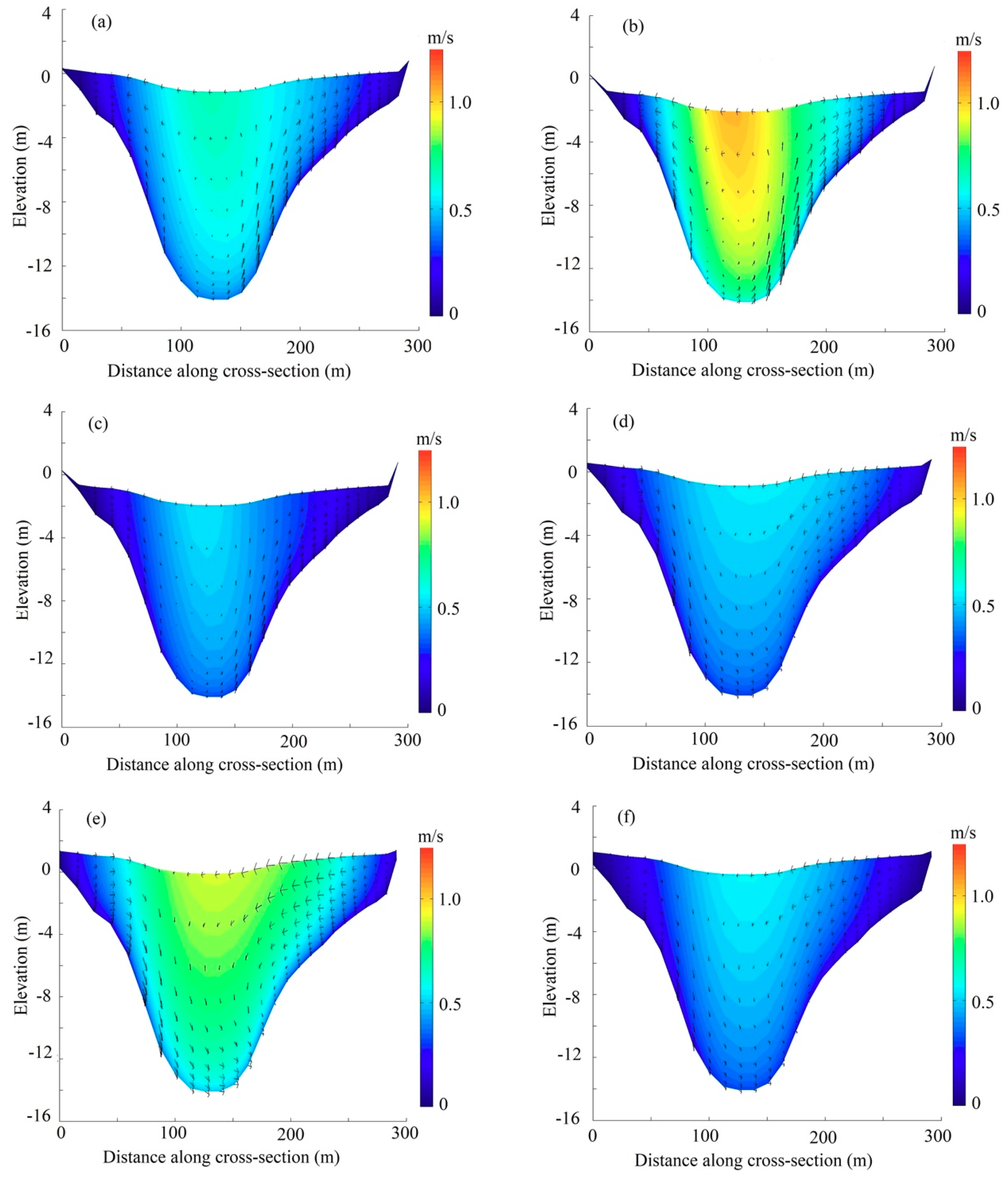
In addition to cross-sectional and streamwise changes of bed forms, the flow patterns in cross-section are also influenced by the rise and fall of the tides, which is different from non-tidal situations with only run-off. Cross-section WL5 is at the bend apex and is chosen to illustrate the issue. Figure 11 shows, during the spring tide, its patterns of the falling period (a,b), low water slack (c), rising period (d,e) and high water slack (f), respectively. Major flow patterns are summarized below:

(1)

During the tidal fall and rise, the cross-sectional flows behave differently in direction and magnitude. For the former, the flow moves from the main stream of higher velocity toward the banks. For the latter, the cross-sectional currents are driven in the opposite direction; the water flowing from the banks are likely to offset each other. The alternating flow causes deposition or erosion at a bend.

(2)

At the low and high water slacks, as shown in Figure 11c,f, the flow strength decreases to its minimum. The reason is that the motion reverses in the subsequent changes, so that the residual motion from the previous tide counteracts the motion in the next period.

(3)

At the bend apex, secondary circulations in cross-section do not occur as commonly observed in non-tidal meandering rivers [4,6]. The difference is mainly ascribed to the tidal level changes, resulting in cross-sectional currents moving away from or toward the streamwise mainstream.

(4)

At the maximum ebb and flood tides, the flow velocity of the mainstream reaches its peak, amounting to 0.8−1.0 m/s and 0.5−0.8 m/s (Figure 11b,e). The former is some 0.2 m/s larger than the latter, which is due to the addition of the ebb tide to the run-off. For the flood tide, the run-off and the tide run in the opposite direction, thus offsetting each other. It holds true that the velocity of the ebb tide is higher than that of the flood tide.

(5)

The flow along the outer bank, during the falling period, is much stronger than that along the inner bank. With the rising tide, the flow pattern shifts and the flow along the inner bank becomes stronger instead. Along the banks in a bend, the opposing and offsetting flows are also visualised by Fenies and Faugeres [28].

In summary, dependent on the rise and fall of the tides, the cross-sectional flow patterns in a meander differ in both flow direction and magnitude. Relative to the main stream, the major feature is an outward movement of water with the falling tide and an inward movement with the rising tide.

6.2. Bed Shear Stress Distribution

For the flood and ebb tides, the bed shear stress ($\overrightarrow{{\tau }_b}$) is useful to judge flow regime and to interpret the resulting patterns of deposition and erosion. For 3D flows, $\overrightarrow{{\tau }_b}$ is expressed in terms of a quadratic function of the $\overrightarrow{u_b}$ and a drag coefficient [22,29].

$$\overrightarrow{{\tau }_b}=\frac{{\rho }_{0}g\overrightarrow{u_b}\left|\overrightarrow{u_b}\right|}{C_{3D}{}^2}$$

(12)

where $\overrightarrow{u_b}$ (m/s) = horizontal velocity in the first layer above the river bed and C_3D = a 3D-Chézy coefficient. For a relatively wide and shallow river, $C_{3\mathrm{D}}=\sqrt[6]{H}/n$.

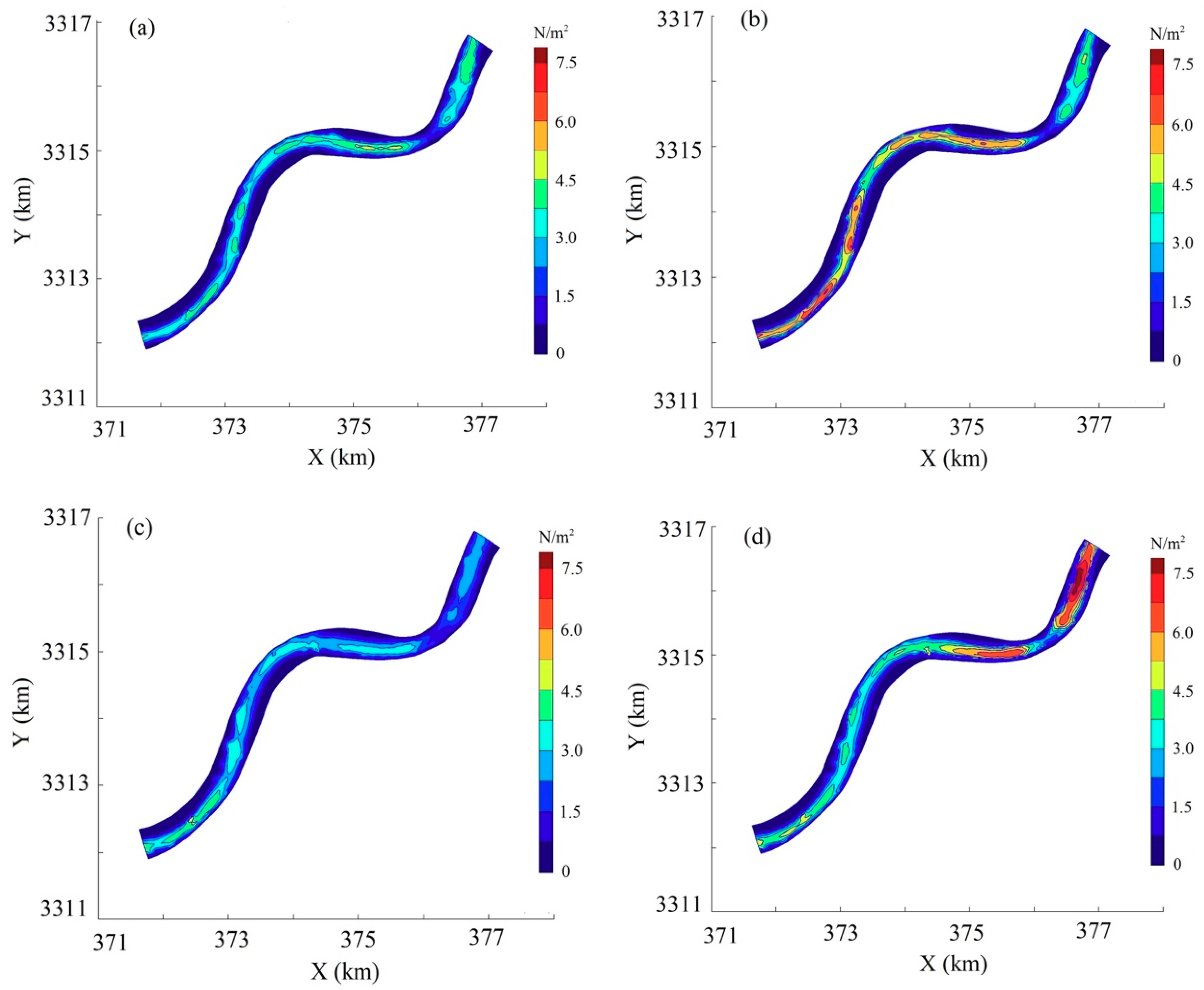
Determination of $\overrightarrow{{\tau }_b}$ is influenced by such factors as river curvature, cross-sectional asymmetry and sediment composition, etc. Due to flow perturbations, it is not straightforward to directly measure it in the field. Numerical modeling is employed for its analysis of the meandering stream. For the wet season (June 2015), Figure 12 displays $\overrightarrow{{\tau }_b}$ distributions at four instants, i.e., (a) high water, (b) maximum ebb tide, (c) low water and (d) maximum flood tide. $\overrightarrow{{\tau }_b}$ varies with discharge, bend curvature, cross-sectional asymmetry, etc., demonstrating the following features.

(1)

$\overrightarrow{{\tau }_b}$ is proportional to $\overrightarrow{u_b}\left|\overrightarrow{u_b}\right|$ and is also a function of H. In the meander reach, the $\left|\overrightarrow{u_b}\right|$ and H values are between 0.2–0.6 m/s and 6.0–14.0 m (exclusive of the scour hole at WL5). At the low and the high water, a similar $\overrightarrow{{\tau }_b}$ distribution is exhibited (Figure 12a,c), with minor local discrepancy. $\overrightarrow{{\tau }_b}$ reflects the velocity gradient, governed by the run-off and tides. At the maximum ebb and flood tides, the peak $\overrightarrow{{\tau }_b}$ values are shown in Figure 12b,d.

(2)

Due to erosion, a deep hole exists at bend apex WL5. Its $\overrightarrow{{\tau }_b}$ distribution features low values. This is ascribed to the large water depth. Shoaling areas along the inner banks show always low $\overrightarrow{{\tau }_b}$ values.

(3)

The spatial distribution is also affected by the curvature. A salient feature is, following the main stream, a band of high $\overrightarrow{{\tau }_b}$ values. In the flow direction, it shifts from the outer bank in one bend to the outer bank in the subsequent bend. This is true for both flood and ebb tides. The occurrence of the band is similar to the situation with a non-tidal meander reach [30,31].

6.3. Sediment Carrying Capacity

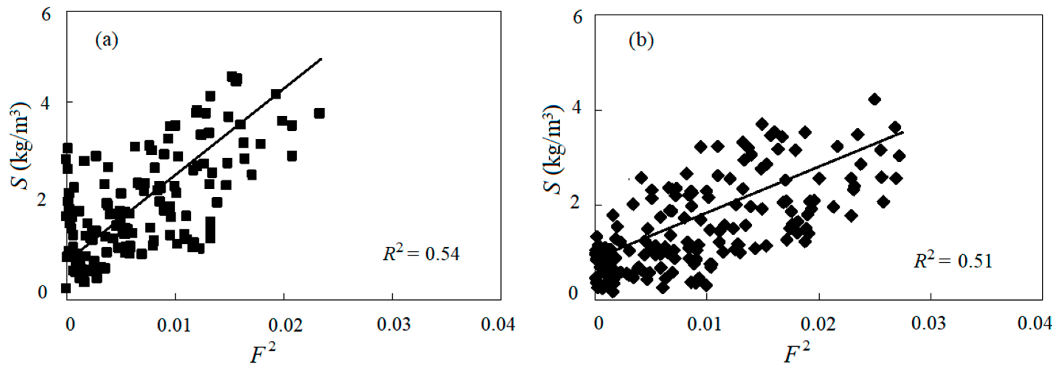
The sediment carrying capacity (S_c, kg/m³) reflects, as an index, the amount of entrained sediment transported by the flow if erosion and deposition are in equilibrium. In comparison with the actual S in the water, predictions are made of morphological changes. If S > S_c, the flow is over-saturated with sediment and deposition occurs. If S < S_c, it is under-saturated, and erosion takes place. S_c is shown to have a linear relationship with F² (Froude number F = V²/(gH)) [17,32,33], with the following expression

$$S_c=S_0+ƒ\left(F^2\right)=S_0+k{F}^2$$

(13)

where k = coefficient and S₀ = background sediment concentration, i.e., the amount of sediment left from the previous tide. The multivariate linear regression analysis and the least square method are used for their estimations. At each time interval, a cross-section has 3 × 6 = 18 measured values. For the 30-h measurement period, 30 sets of the data are analysed. For the flood and ebb tides of the wet season in June 2015, Figure 13 shows the obtained S–F² relationship.

The S_c expression for the meander reach is written as

$$\mathrm{Flood}\mathrm{tide},S_c=103.86F^2+1.09$$

(14)

$$\mathrm{Ebb}\mathrm{tide},S_c=58.67F^2+0.92$$

(15)

The k value for the flood tides is almost twice as high as for the ebb tides. It is, therefore, reasonable to separately determine S_c—the former carries more sediment than the latter. Chen et al. [17,32] examined S_c during wet and dry seasons, which also show significantly different S_c values.

In a meander subjected to the interaction of run-off and tides, S_c depends on a few factors and shows its complexity in both time and space. In consideration of the nature of the issue, it is not straightforward to find a unified S_c formula with accuracy. Though there are other forms of expressions, the commonly accepted expression is based on F, implying that S_c is mainly dependent on turbulence intensity [33,34].

6.4. Erosion-Deposition Patterns

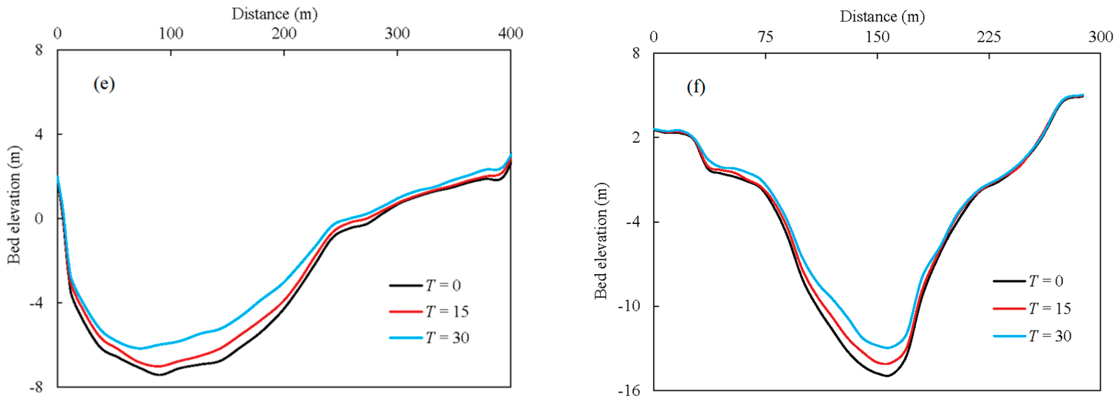
Predictions are made to look at the potential sediment patterns in the meander. The tidal currents, especially the spring tide in a wet season, dominate the sediment transport. During the 2nd half of June 2015, the 30-h spring tide is chosen for the purpose, corresponding to a critical scenario of interest. Compared with river flow conditions, morphological changes are a slower process. When only simulating a 30-hr period, changes in the bed level are hardly noticeable. A morphological scaling factor is thus used to amplify the bed-form change, a method of common practice [21,35,36]. It is set to 24, leading to a one-month prediction. A longer time series of measured sediment data is not available.

The start condition corresponds to the measured bathymetry at 10:00 on 17 June 2015. Figure 14a−c illustrates the bed-form evolution from T = 0, 15 to 30 days. As time elapses, the results show that, except for the slight erosion in the vicinity of WL4, gradual deposition features the meander reach. The trend is in qualitative agreement with the observation made by Chen et al. [17,32], in which the influence of the wading structures, including bridges and wharfs, was also included. Figure 14d−f illustrates, as a function of time, the cross-sectional bed profiles at WL4, FS4 and WL5.

For a given cross-section, its inner bank is exposed to heavier deposition than the outer bank. The mainstream tends to switch more to the outer bank, aggravating the curvature of the bend.

During a tidal circle, sediment transport into and out of the reach is not in balance, leading to sediment storage along the reach. As shown in the field measurements, the flood tide carries more sediment and results in deposition. For an ebb tide, its low bed shear stress can only re-suspend a limited amount of the deposited sediment from the flood tides, only slight erosion occurs. The flood tide plays a dominant role. An oblong scour hole exists at WL5. At maximum, its hole depth is initially 14.0 m and becomes 13.05 m at T = 30 days. The hole shrinks both up- and downstream as time elapses. Both the flood and ebb tides contribute to shaping the scour hole.

Sediment deposition occurs easily around the flow reversal, i.e., the shift between flood and ebb tides, which is dependent on the duration of slack waters. As shown earlier (Figure 11c,e), the cross-sectional flow momentum during the slacks decreases to a minimum. The offsetting effect between the flood tide and run-off results in a long slack duration around the high water. As a result, more suspended sediment settles at the reversals.

To sum up, the flow regime and imbalance of sediment transport are the main drivers of the meander reach evolution. Though there is no complete bathymetry data available to calibrate the morphological change for the reach, the simulation suggests that the bed-level changes are closely related to the interactions between the run-off and tides. The latter plays a dominating role and governs the sedimentation.

7. Conclusions

If river run-off and strong tides co-exist in a meander reach, its flow and morphological changes are governed by several factors and exhibit both spatial and periodical changes. Field and numerical studies are made to examine such a tidal meander reach.

Field measurements show that approximately 95% of the river sediment is suspended load, most of which is transported upstream into the reach by the flood tides, especially during the spring-tide period. Tidal currents stir sediment and modify its concentration, which leads to the fact that the flow velocity and sediment concentration are out of phase with one another. The asymmetry in cross-section and bi-directional flow affect the re-distribution of suspended load, leading to a higher concentration in the inner banks than in the outer banks. Additionally, the near-bottom values are usually 2−5 times the surface ones. Based on the extensive filed data, a formula of sediment carrying capacity is formulated as a function of the Froude number, with which deposition and erosion patterns can be judged.

Based on the Delft3D software, a 3D model of suspended sediment transport is setup to simulate the alluvial behavior of the reach. The flow exhibits significant vertical stratifications; the velocity distribution differs from the logarithmic profile valid for a non-tidal straight river reach. During the tidal rise and fall, the cross-sectional flow moves in the opposite direction. At the water slacks, the momentum decreases to a minimum. Sediment settles mainly during the flow reversal and the durations of slack water affects the deposited amount. The spatial distribution of the bed shear stress follows the pattern of velocity gradient and is also affected by the meander asymmetry.

With a morphological scale factor, the bed-form change of the meander reach is predicted. The results show that, during a tidal circle, the suspended load transport in and out of the reach is not in balance and gives rise to gradual siltation, which is mainly owing to the flood tides that carry most of the load. The offsetting effect between the flood tide and run-off results in a long slack duration around the high water, facilitating the sediment deposition when the current reverses between the flood and ebb tides.

The tides interact with the fresh-water run-off and lead to varied sediment patterns in space and time, generating a different morphological regime from a non-tidal meander reach. The study, especially the collected field data, contributes to the understanding of the fluvial behaviors and is of reference to other investigations of similar tidal meander rivers.

References

- Da Silva, A.M.F.; Ebrahimi, M. Meandering morphodynamics: Insights from laboratory and numerical experiments and beyond. J. Hydraul. Eng. 2017, 143, 3117005. [Google Scholar] [CrossRef]
- Blanckaert, K.; de Vriend, H.J. Turbulence structure in sharp open-river bends. J. Fluid Mech. 2005, 536, 27–48. [Google Scholar] [CrossRef]
- Fong, D.A.; Monismith, S.G.; Stacey, M.T.; Burau, J.R. Turbulent stresses and secondary currents in a tidal-forced river with significant curvature and asymmetric bed forms. J. Hydraul. Eng. 2009, 135, 198–208. [Google Scholar] [CrossRef]
- Feurich, R.; Olsen, N.R.B.; Asce, M. Three-dimensional modeling of nonuniform sediment transport in an S-shaped river. J. Hydraul. Eng. 2011, 137, 493–495. [Google Scholar] [CrossRef]
- Lacy, J.R.; Monismith, S.G. Secondary currents in a curved, stratified, estuarine channel. J. Geophys. Res. 2001, 106, 31283–31302. [Google Scholar] [CrossRef] [Green Version]
- Stoesser, T.; Ruether, N.; Olsen, N.R.B. Calculation of primary and secondary flow and boundary shear stresses in a meandering river. Adv. Water Resour. 2010, 33, 158–170. [Google Scholar] [CrossRef]
- Fischer-Antze, T.; Rüther, N.; Olsen, N.R.B.; Gutknecht, D. Three-dimensional (3D) modeling of non-uniform sediment transport in a river bend with unsteady flow. J. Hydraul. Res. 2009, 47, 670–675. [Google Scholar] [CrossRef]
- Da Silva, A.M.F. Turbulent Flow in Sine-Generated Meandering Rivers. Ph.D. Thesis, Queen’s University, Kingston, ON, Canada, 1995. [Google Scholar]
- Abad, J.D.; Garcia, M.H. Experiments in a high-amplitude Kinoshita meandering river: 1. Implications of bend orientation on mean and turbulent flow structure. Water Resour. Res. 2009, 45, W02401. [Google Scholar]
- Abad, J.D.; Garcia, M.H. Experiments in a high-amplitude Kinoshita meandering river: 2. Implications of bend orientation on bed morphodynamics. Water Resour. Res. 2009, 45, W02402. [Google Scholar]
- Termini, D.; Piraino, M. Experimental analysis of cross-sectional flow motion in a large amplitude meandering bend. Earth Surf. Process. Landf. 2011, 36, 244–256. [Google Scholar] [CrossRef]
- Rippeth, T.P.; Simpson, J.H.; Williams, E.; Inall, M.E. Measurement of the rates of production and dissipation of turbulent kinetic energy in an energetic tidal flow: Red wharf bay revisited. J. Phys. Oceanogr. 2003, 33, 1889–1901. [Google Scholar] [CrossRef]
- Olsen, N.R.B. Three-dimensional CFD modeling of self-forming meandering river. J. Hydraul. Eng. 2003, 129, 366–372. [Google Scholar] [CrossRef]
- Hsieh, T.; Yang, J. Investigation on the suitability of two-dimensional depth-averaged models for bend-flow simulation. J. Hydraul. Eng. 2003, 129, 597–612. [Google Scholar] [CrossRef]
- Zhu, H.; Wang, L.L.; Tang, H.W. Large-eddy simulation of suspended sediment transport in turbulent river flow. J. Hydrodyn. (Ser. B) 2013, 25, 48–55. [Google Scholar] [CrossRef]
- Koken, M.; Constantinescu, G.; Blanckaert, K. Hydrodynamic processes, sediment erosion mechanisms, and Reynolds-number-induced scale effects in an open river bend of strong curvature with flat bathymetry. J. Geophys. Res. Earth Surf. 2013, 118, 2308–2324. [Google Scholar] [CrossRef]
- Chen, J.; Tang, H.W.; Xiao, Y.; Ji, M. Hydrodynamic characteristics and sediment transport of a tidal river under influence of wading engineering groups. China Ocean Eng. 2013, 27, 829–842. [Google Scholar] [CrossRef]
- Shen, C.L. The fluvial processes of the Yongjiang River and its channel regulation (in Chinese). Geophys. Res. 1988, 7, 58–66. [Google Scholar]
- Xie, Q.C.; Yang, J.; Lundström, S.; Dai, W.H. Understanding morphodynamic changes of a tidal river confluence through field measurements and numerical modeling. Water 2018, 10, 1424. [Google Scholar] [CrossRef]
- Wang, Z.Y.; Lee, J.H.W.; Melching, C.S. River Dynamics and Integrated River Management, 1st ed.; Tsinghua University Press: Beijing, China, 2014; pp. 13–16. ISBN 978-7-302-27257-1. [Google Scholar]
- Ranjan, A.; Ray, B.K. Mathematical modelling of sediment transport in estuaries. Estuar. Process. 1977, 98–106. [Google Scholar] [CrossRef]
- Deltares. Delft3D-Flow, User Manual; Deltares: Delft, The Netherlands, 2014. [Google Scholar]
- Partheniades, E. Erosion and deposition of cohesive soils. J. Hydraul. Div. 1965, 91, 105–139. [Google Scholar]
- Emmanuel, P. Turbidity and cohesive sediment dynamics. Elsevier Oceanogr. Ser. 1986, 42, 515–550. [Google Scholar]
- Lesser, G.R.; Roelvink, J.A.; van Kester, J.A.T.M.; Stelling, G.S. Development and validation of a three-dimensional morphological model. Coast. Eng. 2004, 51, 883–915. [Google Scholar] [CrossRef]
- Moriasi, D.N.; Arnold, J.G.; Van Liew, M.W.; Bingner, R.L.; Harmel, R.D.; Veith, T.L. Model evaluation guidelines for systematic quantification of accuracy in watershed simulations. Trans. ASABE 2007, 50, 885–900. [Google Scholar] [CrossRef]
- Krause, P.; Boyle, D.P.; Bäse, F. Comparison of different efficiency criteria for hydrological model assessment. Adv. Geosci. 2005, 5, 89–97. [Google Scholar] [CrossRef] [Green Version]
- Fenies, H.; Faugeres, J.C. Facies of geometry of tidal channel-fill deposits (Arcachon Lagoon, SW France). Mar. Geol. 1998, 150, 131–148. [Google Scholar] [CrossRef]
- Collins, M.B.; Ke, X.; Gao, S. Tidally-induced flow structure over intertidal flats. Estuar. Coast. Shelf Sci. 1998, 46, 233–250. [Google Scholar] [CrossRef]
- Robert, A. River Processes, 1st ed.; Hodder Education: London, UK, 2003; pp. 132–142. ISBN 978-0-340-76339-1. [Google Scholar]
- Engel, F.L.; Rhoads, B.L. Three-dimensional flow structure and patterns of bed shear stress in an evolving compound meander bend. Earth Surf. Process Landf. 2016, 41, 1211–1226. [Google Scholar] [CrossRef]
- Chen, J.; Ji, M.; Zhang, H.J.; Yan, W.W.; Tang, H.W. Analysis of water and sediment characteristics during flood and low water period of Yong River (in Chinese). Hydro-Sci. Eng. 2012, 5, 48–54. [Google Scholar]
- Zheng, J.; Li, R.J.; Yu, Y.H.; Suo, A.N. Influence of wave and current flow on sediment-carrying capacity and sediment flux at the water–sediment interface. Water Sci. Technol. 2014, 70, 1090–1098. [Google Scholar] [CrossRef]
- Engelund, F.; Hansen, E. Comparison between Similarity Theory and Regime Formulae; Basic Research-Progress Report 13; Hydraulic Laboratory, Technical University of Denmark: Lyngby, Denmark, 1967. [Google Scholar]
- Briere, C.; Giardino, A.; van der Werf, J. Morphological modeling of bar dynamics with Delft3D: The quest for optimal free parameter settings using an automatic calibration technique. Coast. Eng. Proc. 2011, 1, 60. [Google Scholar] [CrossRef]
- Moerman, E. Long-Term Morphological Modeling of the Mouth of the Columbia River. Master’s Thesis, Delft University of Technology, Delft, The Netherlands, 2011. [Google Scholar]
Figure 1.
Study area: (a) Location; (b) examined meandering reach of the Yong River; (c) measurement stations of water levels (WL) and flow & sediment (FS).
Figure 2.
Geometrical description of the meander, with flow and sediment stations FS3, FS4 and FS5. Each bend is described with a center position O, a radius R and an angle θ. The red line denotes the central line throughout the reach.
Figure 3.
Schematic diagram of cross-sectional measurement points (looking downstream).
Figure 4.
S distributions of lines A, B and C at each FS during the wet season (2nd half of June 2015).
Figure 5.
Distributions of along lines A, B and C at FS4 during the wet season: (a) Spring tide; (b) Neap tide.
Figure 6.
Relationship between V and S at FS5: (a) Spring tide; (b) Neap tide.
Figure 7.
Numerical grids: (a) A coarse grid over the domain; (b) Local refinement in the vicinity of WL5; (c) Local refinement upstream of WL6.
Figure 8.
Measured Q, Z and S as boundary conditions: (a) Q~t and Z~t; (b) S~t.
Figure 9.
Model calibration with measured versus predicted for the spring tide (June 2015): (a) Z at WL4; (b) Z at WL5; (c) V at FS4; (d) S at FS4.
Figure 10.
Model validation with the neap tide (June 2015): (a) Z at WL4; (b) Z at WL5; (c) V at FS4; (d) S at FS4.
Figure 11.
Cross-sectional flow patterns during the spring tide: (a,b) Falling period; (c) Low water slack; (d,e) Rising period; and (f) High water slack.
Figure 12.
Distributions of during the wet season (June 2015): (a) High tide; (b) Maximum ebb tide; (c) Low tide; (d) Maximum flood tide.
Figure 13.
S–F2 relationship for the wet season (June 2015): (a) Flood tides; (b) Ebb tides.
Figure 14.
Morphological changes during the spring tide: (a) T = 0 (measured bed level); (b) T = 15 days; (c) T = 30 days; cross-sectional bed level changes at (d) WL4; (e) FS4; (f) WL5.