Article

Eddy Backscatter and Counter-Rotating Gyre Anomalies of Midlatitude Ocean Dynamics

Department of Mathematics, Imperial College London; Huxley Building, 180 Queen’s Gate, London SW7 2AZ, UK
*
Author to whom correspondence should be addressed.
Fluids 2016, 1(3), 28; https://doi.org/10.3390/fluids1030028
Submission received: 14 May 2016 / Revised: 18 August 2016 / Accepted: 25 August 2016 / Published: 2 September 2016
(This article belongs to the Collection Geophysical Fluid Dynamics)

Abstract

:
This work concerns how two competing mechanisms—eddy backscatter and counter-rotating gyre anomalies—influence the midlatitude ocean dynamics, as described by the eddy-resolving quasi-geostrophic (QG) model of wind-driven gyres. We analyzed dynamical balances and effects of different eddy forcing components, as well as their dependencies on increasing vertical resolution and decreasing eddy viscosity and found that the eastward jet and its adjacent recirculation zones are maintained mostly by the eddy forcing via the eddy backscatter mechanism, whereas the time-mean eddy-forcing component plays not only direct jet-supporting but also indirect jet-inhibiting role. The latter is achieved by inducing zonally elongated anticyclonic/cyclonic Counter-rotating Gyre Anomaly (CGA) in the subpolar/subtropical gyre. The indirect effect of CGAs on the eastward jet is found to be moderate relative to the dominant eddy backscatter mechanism. We also found that the higher the vertical baroclinic mode, the weaker its backscatter role and the stronger its CGA-driving role. Although the barotropic and first baroclinic modes are the most efficient ones in maintaining the backscatter, the higher, up to the fifth baroclinic modes also have significant but reverse impact that reduces the backscatter.

1. Introduction

Dynamics of the large-scale ocean circulation is tackled from various perspectives ranging from theoretical analyses of light, process-oriented problems to extremely large computations of comprehensive ocean general circulation models (OGCMs) (e.g., [1,2,3]). In this paper, we examine the double-gyre QG model in three-, six-, and twelve-layer configurations and study how the time-mean nonlinear stresses and the transient eddy forcing affect the large-scale circulation. Being process-oriented and computationally inexpensive relative to modern OGCMs, the QG model allows to analyze eddy-resolving flow regimes for a wide range of parameters. In the past QG studies helped to understand various effects of mesoscale eddies (e.g., [4,5]), patterns arising from early bifurcations (e.g., [6,7,8,9]), coupling with the atmosphere (e.g., [10]), and other aspects of flow dynamics.
A rare study of the influence of vertical resolution on the eastward jet extension is [11], where the authors were focused on the eddy-permitting three- and six-layer QG double gyres and concluded that the third and higher baroclinic modes play a catalytic role resulting in the nonlinear amplification of the eastward jet. Another series of works [12,13] studied more idealized, horizontally homogeneous, eddy-resolving QG dynamics and found that for the ocean-like stratification the kinetic energy is transferred from high baroclinic modes through the first baroclinic mode to the barotropic one. Although, the impact of the horizontal resolution on the flow dynamics was extensively studied in QG double gyres (e.g., Shevchenko and Berloff [14]) and to some extent in comprehensive OGCMs (e.g., Kirtman et al. [15]), no works have attempted a systematic study of the nonlinear eddy effects and mechanisms in the idealized eddy-resolving model, and as a function of increasing vertical resolution and decreasing eddy viscosity. We systematically address these issues in the turbulent double-gyre QG model with focus on the eastward jet extension of the western boundary currents and on the interior gyres.

2. Double-Gyre Model

The double-gyre QG model [16,17] for the evolution of PV anomaly q is considered in three-, six- and twelve-layer configurations (denoted as 3L, 6L and 12L) and given by
t q i + J ψ i , q i + β y = δ 1 i F w δ i N μ Δ ψ i + ν Δ 2 ψ i , 1 i N ,
where J ( f , g ) f x g y f y g x , and δ i j is the Kronecker symbol; N = { 3 , 6 , 12 } is the corresponding number of stacked isopycnal fluid layers with depths given in Table 1, and with both density and index increasing downward. The density changes vertically in accord with the hyperbolic tangent profile that has inflection point at 500 m and width scale of 200 m . The chosen density profile is consistent with our focus on the motions in the permanent thermocline and helps to leave outside of this focus QG motions associated with the surface density anomalies. The computational domain Ω is a square, closed, flat-bottom basin of dimensions L × L × 4 km , with L = 3840 km . The asymmetric wind curl is the forcing (i.e., Ekman pumping) that drives the double-gyre ocean circulation, and it is given by
F w = 1 . 80 π τ 0 sin π y / y 0 , y [ 0 , y 0 ) ,     2 . 22 π τ 0 sin π ( y y 0 ) / ( L y 0 ) , y [ y 0 , L ] ,
with the wind stress amplitude τ 0 = 0 . 3 N · m 2 and tilted zero forcing line y 0 = 0 . 4 L + 0 . 2 x , x [ 0 , L ] ; τ 0 is chosen to ensure a realistically strong eastward jet in all solutions [14]. Note that in the 12L model F w is applied to the first two layers, since H 1 ( 12 ) = H 2 ( 12 ) = 0 . 5 H 1 ( 6 ) . The planetary vorticity gradient is β = 2 × 10 11 m 1 · s 1 , the linear bottom friction parameter is μ = 4 × 10 8 s 1 , and the lateral eddy viscosity ν is a parameter specified for each numerical simulation further below.
The layerwise PV anomaly q i and the velocity streamfunction ψ i are dynamically coupled through the system of elliptic equations:
q i = Δ ψ i ( 1 δ i 1 ) s i 1 ( ψ i ψ i 1 ) ( 1 δ i N ) s i 2 ( ψ i ψ i + 1 ) , 1 i N ,
with the stratification parameters s i 1 , s i 2 chosen so, that the Rossby deformation radii are defined by the values in Table 2. Note that the first Rossby radius ( R d 1 = 40 km ) is the same across all model configurations. System (1)–(2) is augmented with the integral mass conservation constraints [18]:
t Ω ( ψ i ψ i + 1 ) d y d x = 0 , 1 i N 1 ,
with the zero initial condition, and with the partial-slip lateral boundary condition:
nn ψ i α 1 n ψ i = 0 , 1 i N ,
where α = 120 km and n is the normal-to-wall and facing inward unit vector. This condition, which is a simple parameterization of dynamically unresolved near-boundary processes, prescribes the tangential velocity component in terms of the exponential decay law based on the characteristic boundary layer thickness α.
The QG model (1)–(4) is solved on the appropriate grid with the CABARET method [19], which simulates large-Reynolds flow regimes cost-efficiently. For each simulation, the model is spun up from the state of rest for T spin = 20 years until the solution is statistically converged. Then, the solution is computed for another T sim = 40 years and analyzed. To guarantee converged solutions for the eddy viscosities ν = { 100 , 50 } m 2 · s 1 (which are considered in the paper to avoid studying high-viscous regimes with undeveloped dynamics) all our numerical experiments were carried out on the appropriate uniform horizontal grids G = { 257 2 , 513 2 } with the actual space steps 15 km and 7 . 5 km , respectively. We call the solution converged if the l 2 -norm relative difference δ ( f , g ) = g f 2 / f 2 between a coarse- and fine-grid solutions g and f is sufficiently small (less than 5%); the difference is computed for the time-mean solution obtained after an initial spin-up (20 years). We will also use the relative error δ to compare different characteristics of solutions. More details on the solution convergence at these and much smaller values of ν can be found in [14].
As the starting point of our analyses, we decompose the velocity streamfunction into the time-mean ψ ¯ i and fluctuating ψ i components, as ψ i = ψ ¯ i + ψ i , and define some extra notations: the integral of a function f ( x , y ) averaged over the domain Ω is denoted by I Ω ( f ) ; f ¯ j ( N ) stands for a time-mean N-layer solution on the j-th layer, and the difference between two solutions is denoted by [ f ] i j = f i f j .

3. Analyses of the Double-Gyre Solutions

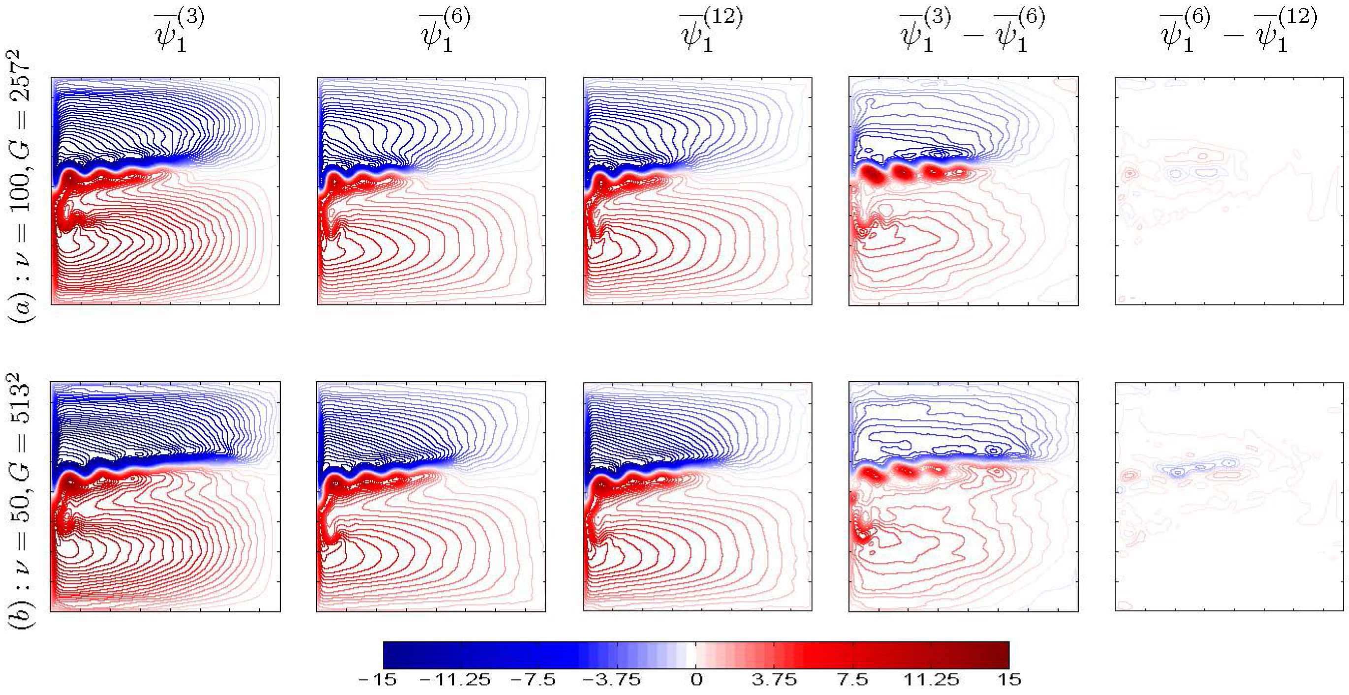
Studying turbulent flow dynamics in process-oriented ocean models with decreasing eddy viscosity, that is with increasing reliance on the explicit eddy dynamics rather than its parameterization, helps to understand the physics and, thus, guide comprehensive general circulation modeling. First, we analyze how the eddy viscosity ν influences the penetration length L p of the eastward jet, (i.e., the distance from the western boundary to the eastern point of the time-mean jet at which the flow velocity drops below 0 . 1 m · s 1 ), the volume transport Q = max i = 1 N ψ ¯ i min i = 1 N ψ ¯ i , and the relative l 2 -norm difference δ between flow fields obtained with different horizontal and vertical resolutions.
As can be seen in Figure 1, the smaller is ν, the stronger is the eastward jet extension and the larger is the volume transport (Table 3); note that L p and Q are larger with fewer layers and smaller ν. The relative difference between 3L and 6L solutions is significant, as illustrated by δ ( ψ ¯ 1 ( 3 ) , ψ ¯ 1 ( 6 ) ) = 0 . 61 ; this difference was computed in the upper layer, where it reaches maximum. However, 6L and 12L solutions are similar on all layers (Figure 2), (e.g., δ ( ψ ¯ 1 ( 6 ) , ψ ¯ 1 ( 12 ) ) = 0 . 05 ), suggesting convergence in terms of the vertical resolution for given value of ν.
Although, it is clear that differences between 3L and 6L solutions are due to the lack of vertical resolution, such an explanation misses the underlying physical mechanism. To address this issue we studied more thoroughly the solutions with ν = 100 m 2 · s 1 , while leaving out (due to the lack of computational resources) similarly detailed analyses of the problem with ν = 50 m 2 · s 1 .

3.1. Eddy Backscatter and Vertical Modes

In this section we study roles of the vertical modes in the main mechanism supporting the eastward jet—the eddy backscatter (see, e.g., [20] in the QG context). We focus on the eddy PV flux divergence, denoted by χ and referred to as the eddy forcing,
χ i = J ψ i , q i J ψ ¯ i , q i J ψ i , q ¯ i , 1 i N ,
and analyse how it affects the large-scale flows.
We considered the time-mean χ ¯ i = J ψ i , q i ¯ and transient χ i = χ i χ ¯ i components of the eddy forcing [21], and, in order to find their dynamical interpretations, carried out numerical experiments discussed further below. Note that χ does not enter the dynamical time-mean balance directly. However, it does so indirectly by driving and controlling the eddy patterns which rectify into the mean flow; our analyses account for this mechanism rather than focus on the less informative time-mean balance. We also decomposed the flow solution into large- and small-scale components and found that the corresponding (and slightly different) χ is systematically correlated with the large-scale eastward jet and enhances it—this is a statistical measure of the eddy backscatter. The simplest way to think about the involved eddy backscatter mechanism is by considering a spatially localized, time-periodic, zero-mean forcing and its dynamical effects [22]: direct contribution of this forcing to the time-mean dynamical balance is zero, nevertheless, it may have an indirect leading-order dynamical effect via systematic correlations with the large-scale flow. It has been shown [4] that at moderate Reynolds numbers this indirect effect provides the main mechanism supporting the eastward jet extension and its adjacent recirculation zones, and here we continue to explore this mechanism at larger Reynolds numbers, with finer horizontal and vertical grid resolutions, and in a more detailed way.
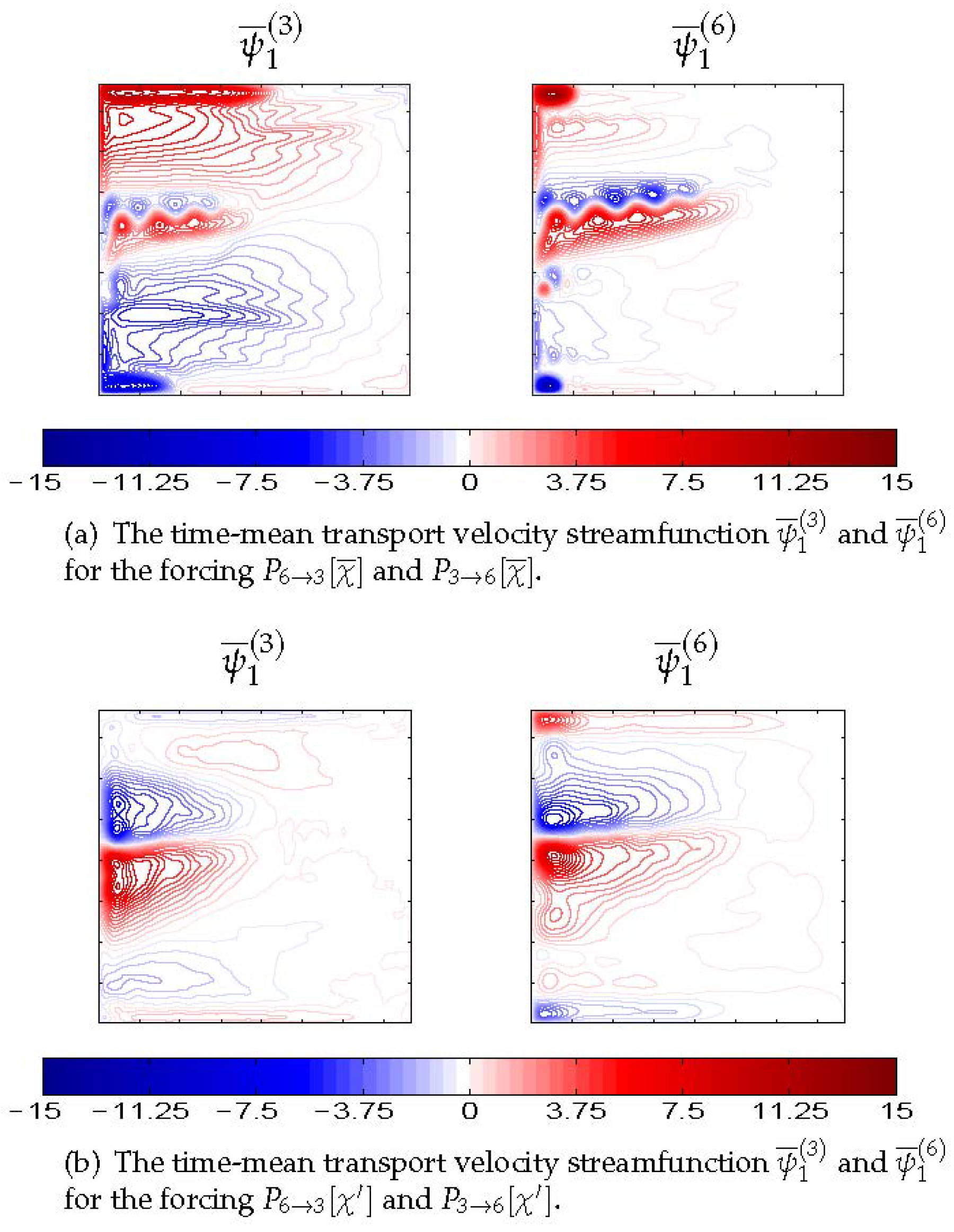
The first series of our numerical experiments (Figure 3) studies dynamical responses to χ ¯ i ( x , y ) and χ i ( x , y , t ) imposed on the state of rest and, thus, provides dynamical interpretation of these eddy forcing patterns. The results show that the eastward jet is induced not only by the time-mean component χ ¯ (Figure 3a) but even more so by the transient component χ (Figure 3b). The latter maintains the eastward jet via positive correlations between the induced jet and χ , similarly to what happens in the full double-gyre circulation. When the flow is forced by χ , the eastward jet length and volume transport are larger in the 3L solution (e.g., Q χ ( 3 ) = 108 Sv and Q χ ( 6 ) = 82 Sv ); here the subscript indicates the force applied. A similar situation is with the volume transport of the flow forced by χ ¯ , i.e., Q χ ¯ ( 3 ) = 135 Sv and Q χ ¯ ( 6 ) = 105 Sv . Thus, we arrive at the important conclusion that the eastward jet and its adjacent recirculation zones are induced not only by the time-mean but more so by the transient eddy forcing, and the jet-maintaining effect weakens with higher vertical resolution.
In fact, the difference between 3L and 6L solutions may be explained by different structures and/or amplitudes of the eddy forcing components. To check this, we projected χ ¯ ( 3 ) and χ ( 3 ) onto the 6L model, and χ ¯ ( 6 ) and χ ( 6 ) onto the 3L model and found the corresponding dynamical responses. In order to do this, we introduced operator P i j , which transforms the i-layer forcing into the j-layer forcing consistently with configurations of the layer depths:
P 3 6 : f 1 ( 3 ) f 1 ( 6 ) , f 2 ( 3 ) f 2 ( 6 ) , f 2 ( 3 ) f 3 ( 6 ) , f 2 ( 3 ) f 4 ( 6 ) , f 3 ( 3 ) f 5 ( 6 ) , f 3 ( 3 ) f 6 ( 6 ) , P 6 3 : f 1 ( 6 ) f 1 ( 3 ) , 1 3 f 2 ( 6 ) + f 3 ( 6 ) + f 4 ( 6 ) f 2 ( 3 ) , 1 2 f 5 ( 6 ) + f 6 ( 6 ) f 3 ( 3 ) .
The responses of the models to P 6 3 [ χ ¯ ] and P 3 6 [ χ ¯ ] ; P 6 3 [ χ ] and P 3 6 [ χ ] (Figure 4) provide dynamical interpretations of the eddy forcings components in terms of the induced large-scale flow responses as functions of vertical resolution. The transformed forcings P 3 6 [ χ ¯ ] , P 3 6 [ χ ] and P 6 3 [ χ ¯ ] , P 6 3 [ χ ] induce similar to the reference solutions structure (Figure 3 and Figure 4). However, the resulting volume transports Q P 6 3 [ χ ¯ ] ( 3 ) = 96 Sv and Q P 3 6 [ χ ¯ ] ( 6 ) = 138 Sv are inhibited and reinforced compared to Q χ ¯ ( 3 ) and Q χ ¯ ( 6 ) , respectively, and more so for the fluctuating parts of the eddy forcing: Q P 6 3 [ χ ] ( 3 ) = 60 Sv and Q P 3 6 [ χ ] ( 6 ) = 170 Sv . Moreover, L p ( 3 ) < L p ( 6 ) for the solution induced by P 6 3 [ χ ] or P 3 6 [ χ ] , which is opposite to the χ -forced case.
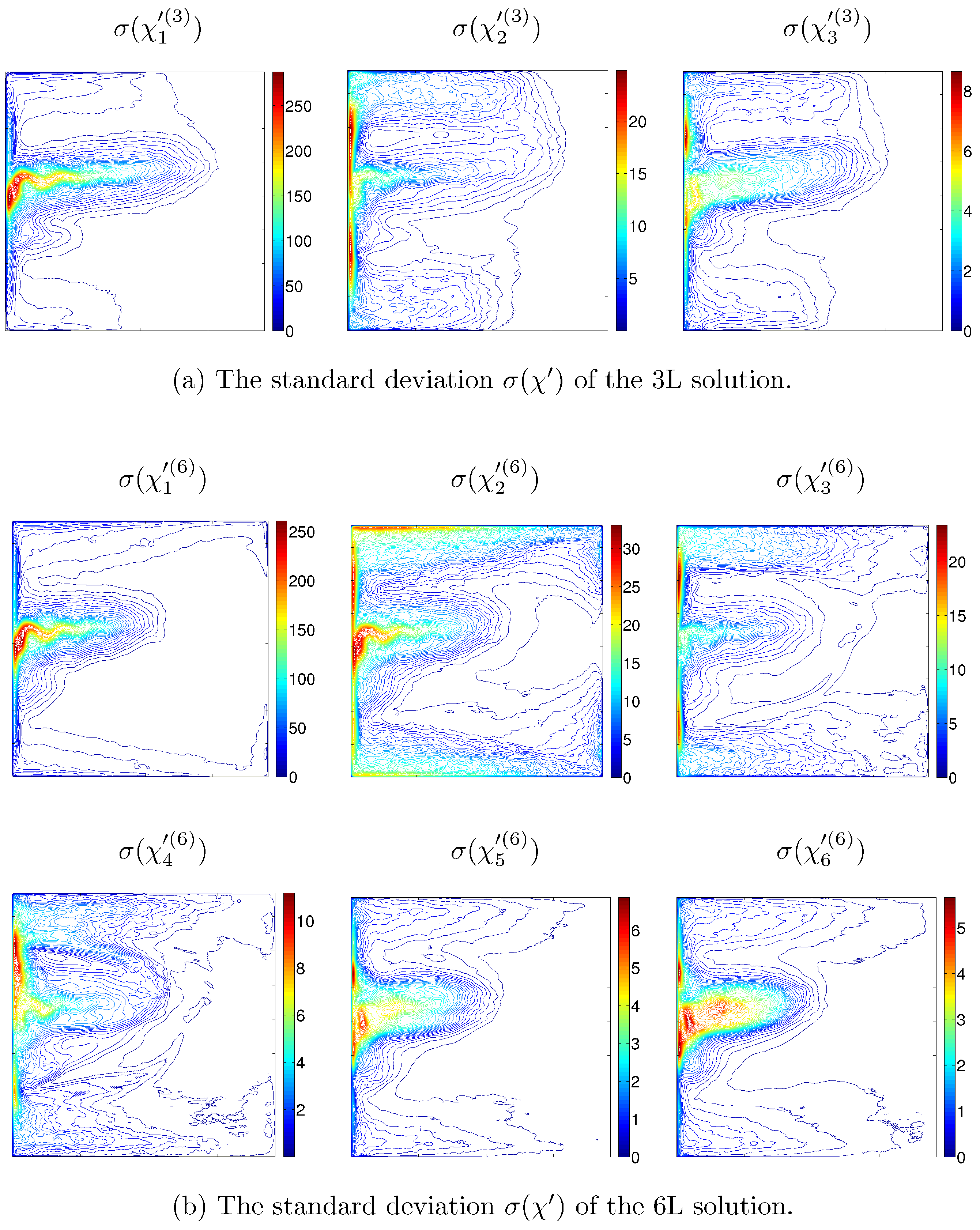
The similarity between the solutions forced by P 6 3 [ χ ] , P 3 6 [ χ ] and by χ ( 3 ) and χ ( 6 ) (as well as by P 6 3 [ χ ¯ ] , P 3 6 [ χ ¯ ] and by χ ¯ ( 3 ) and χ ¯ ( 6 ) ) suggests that the 3L and 6L forces are structurally similar, and only their amplitudes are different. Here, we quantify the amplitude difference in terms of the integrals of the standard deviation of χ (Table 4 and Figure 5). In order to verify the amplitude hypothesis we factored out this difference, normalized the amplitudes of the projected quantities χ ( 3 ) , χ ( 6 ) and computed new forcing fields:
χ ^ i ( 3 ) = σ ( χ i ( 3 ) ) σ ( P 6 3 [ χ i ] ) P 6 3 [ χ i ] , χ ^ i ( 6 ) = σ ( χ i ( 6 ) ) σ ( P 3 6 [ χ i ] ) P 3 6 [ χ i ] , 1 i N .
The results are given in Figure 6. The responses of the 3L and 6L models to the forcings χ and χ ^ are nearly the same (Figure 3b and Figure 6): the volume transports Q χ ^ ( 3 ) = 108 Sv and Q χ ^ ( 6 ) = 77 Sv ; the relative errors are δ Q χ ( 3 ) , Q χ ^ ( 3 ) = 0 . 004 and δ Q χ ( 6 ) , Q χ ^ ( 6 ) = 0 . 06 ; and the eastward jet lengths are L p , χ ( 3 ) L p , χ ^ ( 3 ) and L p , χ ( 6 ) L p , χ ^ ( 6 ) for the solutions induced by the forcing χ and χ ^ , respectively. Thus, we conclude that the key aspect is the difference between the amplitudes of the fluctuating components of the 3L and 6L eddy forcings. The mechanism setting the amplitude of the eddy forcing can be understood in terms of vertical modes. For brevity, we refer to the vertical modes as modes and study efficiencies of their feedbacks.
In order to assess individual contributions of the vertical modes to the eddy backscatter, and, thus, to gain further understanding in dynamical effects of higher vertical resolution, we express the QG Equation (1) in terms of the vertical modes φ. For doing so, we rewrite the system of elliptic Equation (2) in vector form as
q = Δ ψ S ψ ,
where S is the stratification matrix defined for N 2 as
j = 1 N S i j ψ j = s i 2 ψ 1 ψ 2 if i = 1 , s i 1 ψ i ψ i 1 + s i 2 ψ i ψ i + 1 if 1 < i < N , s N 2 ψ N ψ N 1 if i = N ,
with the stratification parameters s i 1 , s i 2 .
Multiplying (5) by some matrix Θ yields
Θ q = Δ Θ ψ Θ S ψ .
The matrix Θ is chosen so that Λ = Θ S Θ 1 , where Λ is the diagonal matrix of the eigenvalues of the stratification matrix S , and columns of Θ 1 are the corresponding eigenvectors of S . Hence, Equation (6) can be rewritten as
Θ q = Δ Θ ψ Λ Θ ψ .
Thus, the QG Equation (1) and velocity streamfunction can be projected from layers ψ = ( ψ 1 , ψ 2 , ψ 3 ) onto modes ϕ = ( ϕ 0 , ϕ 1 , ϕ 2 ) by the linear transformation Θ : ψ ϕ , where ϕ 0 denotes the barotropic mode, and ϕ m > 0 is the m-th baroclinic mode. In fact, the mode ϕ i is the streamfunction representation of the i-th mode. The inverse transformation Θ 1 : ϕ ψ maps the modes back to the layers. We also introduce the selected-mode inverse transformation Θ m 1 , in which all the modes in the inverse mapping, but the m-th one, are set to zero.
In order to study how efficient is eddy forcing of each mode, we define the efficiency of a forcing F (defined further below) applied to the QG model as a ratio between the volume transport of the corresponding flow ψ ¯ F ( i ) (forced with F ) and the reference flow ψ ¯ ( i ) (forced with the constant wind forcing F w ):
E ( i ) ( F ) = Q ( ψ ¯ F ( i ) ) Q ( ψ ¯ ( i ) ) ,
where Q ( · ) is the corresponding volume transport. In other words, the efficiency of forcing F determines the measure of strength of the eastward jet (forced with F ) with respect to the jet forced with F w .
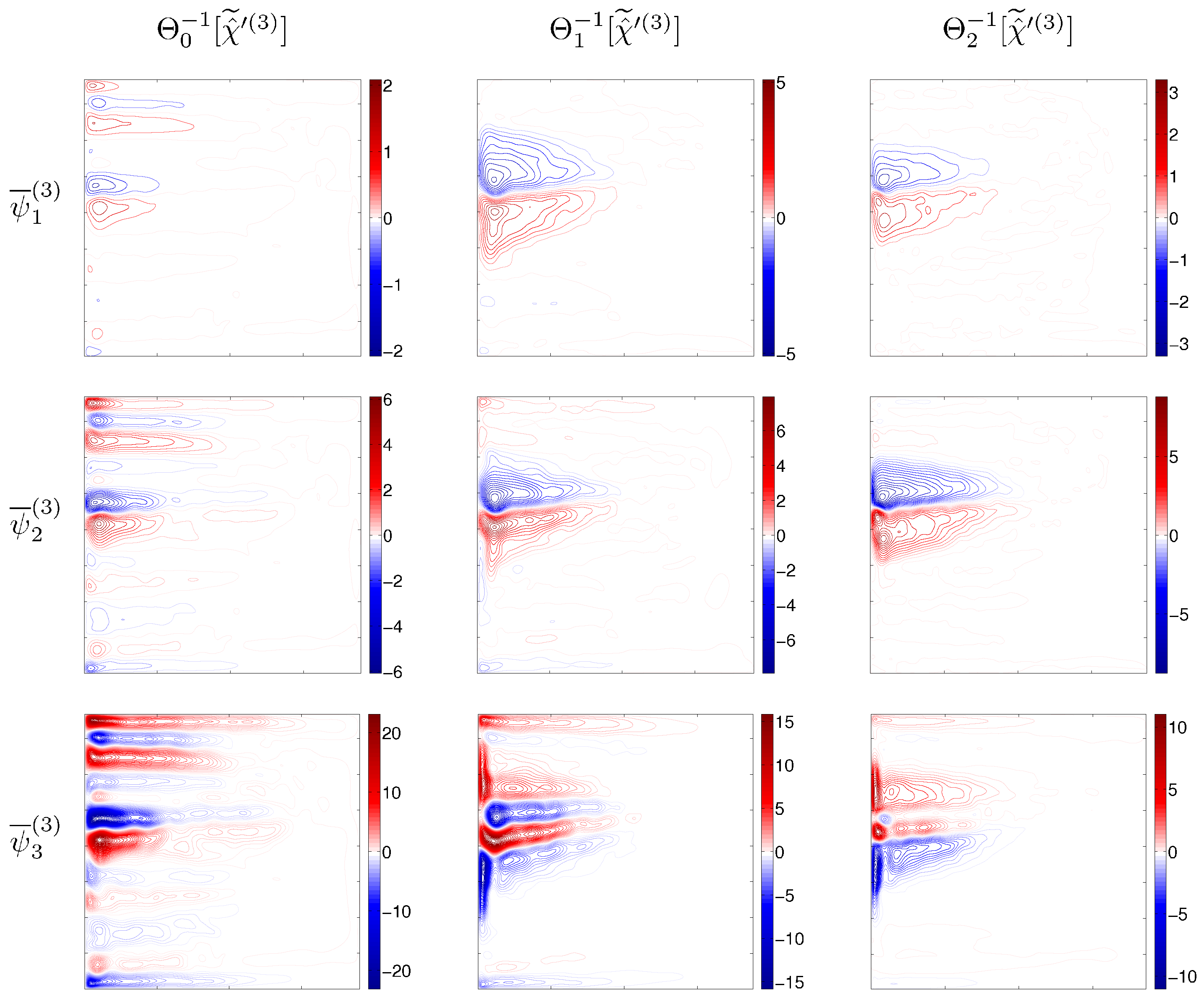
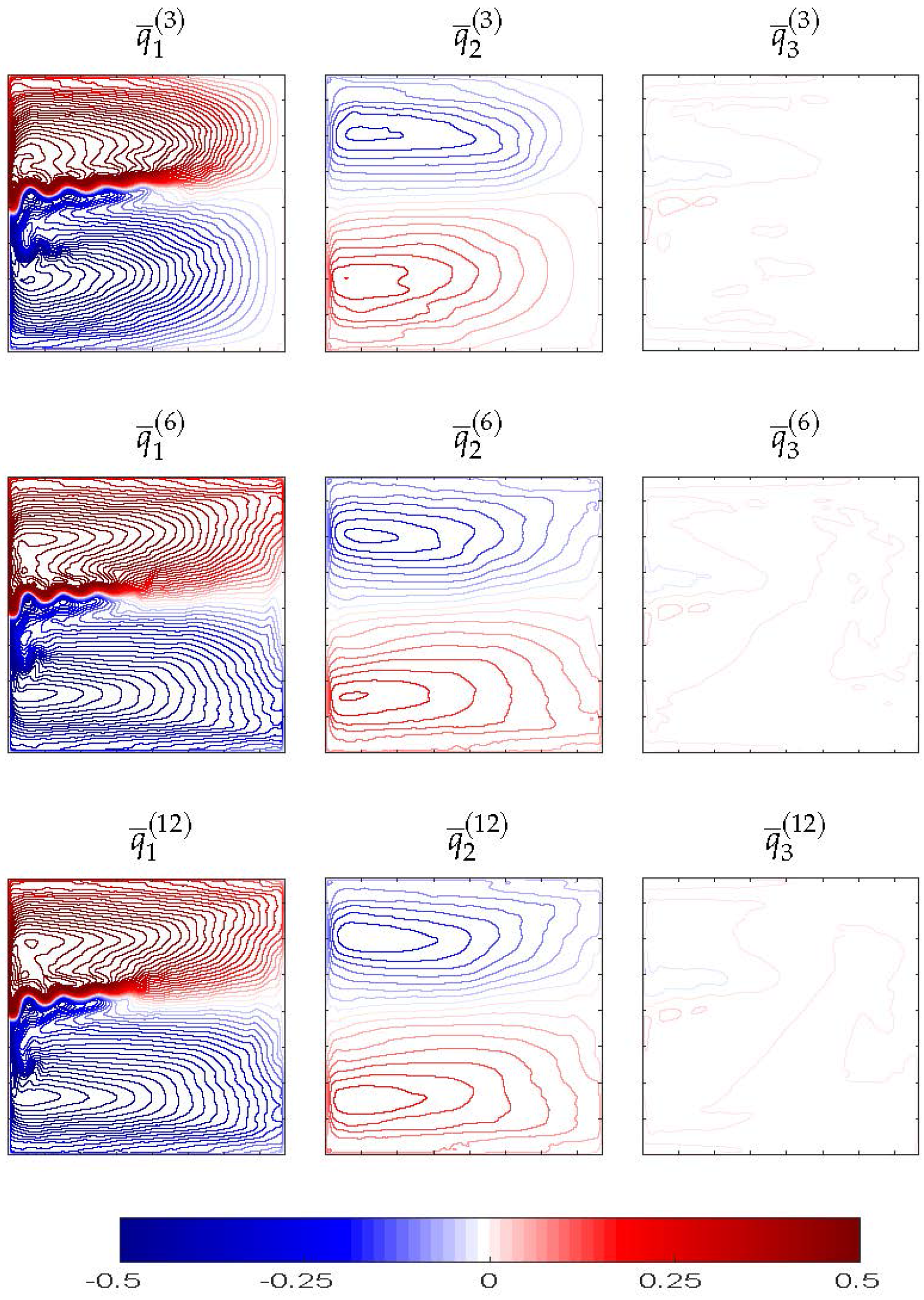
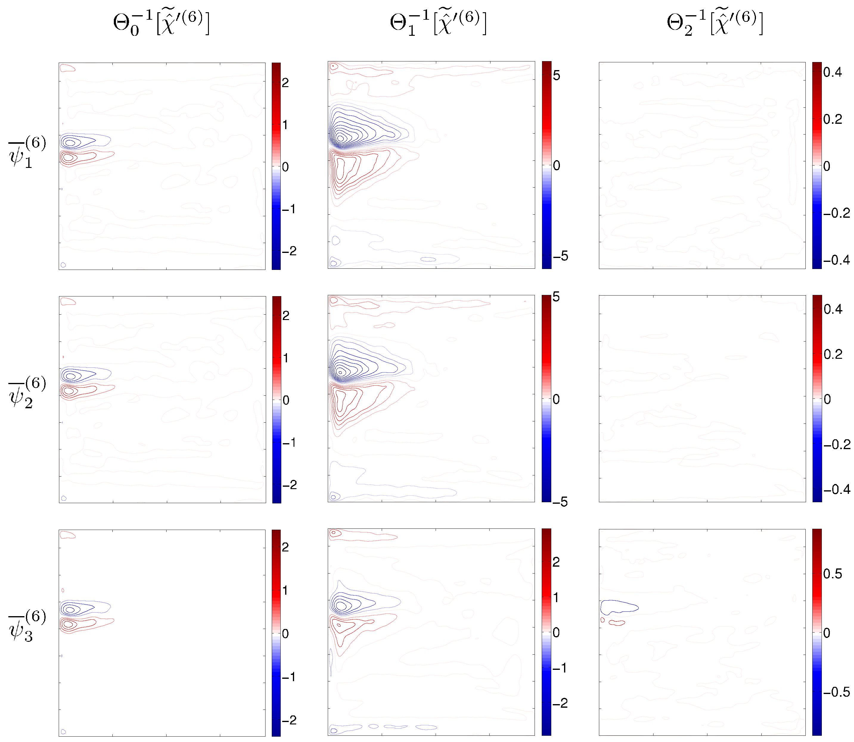
We analyze the 3L and 6L model responses to the selected m-mode forcings Θ m 1 [ χ ^ ˜ ] (the fluctuating component of the eddy forcing χ ^ is firstly projected forward onto the modes and then backward onto the layers, with all the modes, save for the m-th one, set to zero before the backward projection; then, the eddy forcing χ ^ projected onto the layers is used as a forcing in the right hand side of Equation (1)), and found that in the 6L model the barotropic and first baroclinic modes are the most efficient ones (Table 5). Our study also reveals two features common to both models: (a) the higher the mode of the eddy forcing is, the weaker its rectified response (Figure 7 and Figure 8); (b) the barotropic, first and second baroclinic eddy forcing modes are the most efficient ones. As shown in Figure 7, the largest responses to the forcing Θ m 1 [ χ ^ ˜ ] are concentrated in ϕ 1 and ϕ 2 modes, suggesting that they accommodate most of the backscatter, although the resulting amplification of the eastward jet is dominated by ϕ 1 . In the 6L case, ϕ 1 plays similar role, but ϕ 2 has weaker feedback (Figure 8). Overall, we conclude that the 3L model captures the quantitative dynamics of the eastward jet but significantly overestimates its strength. Finally, we confirm that all 3L/6L differences are due to the nonlinear eddy effects, because the corresponding linear solutions are nearly the same (Section 3.2).
The eddy backscatter is not the only mechanism taking part in the nonlinear dynamics of the eastward jet. In the next section, we study another important mechanism which works against the backscatter (i.e., inhibits the eastward jet).

3.2. Counter-Rotating Gyre Anomalies

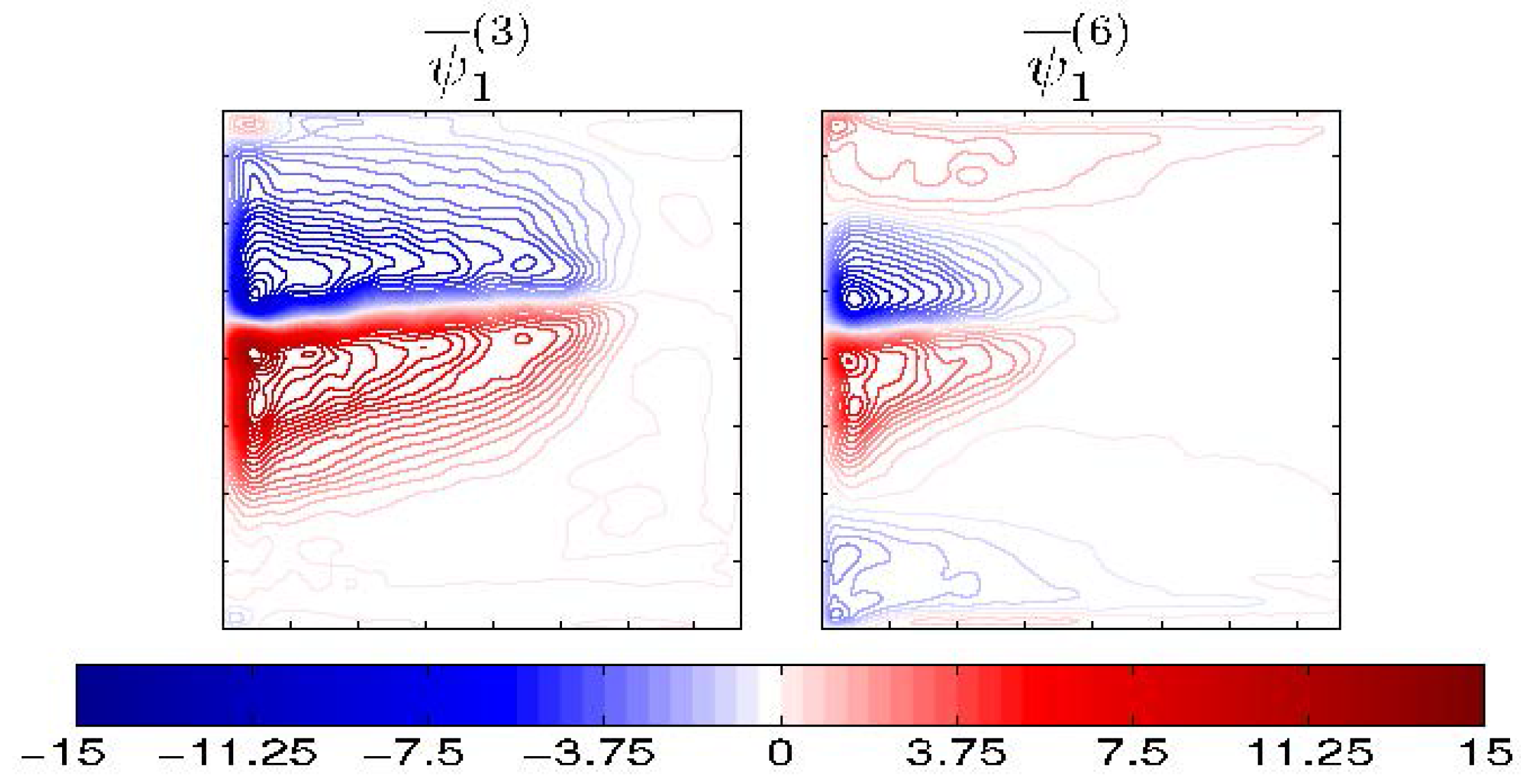
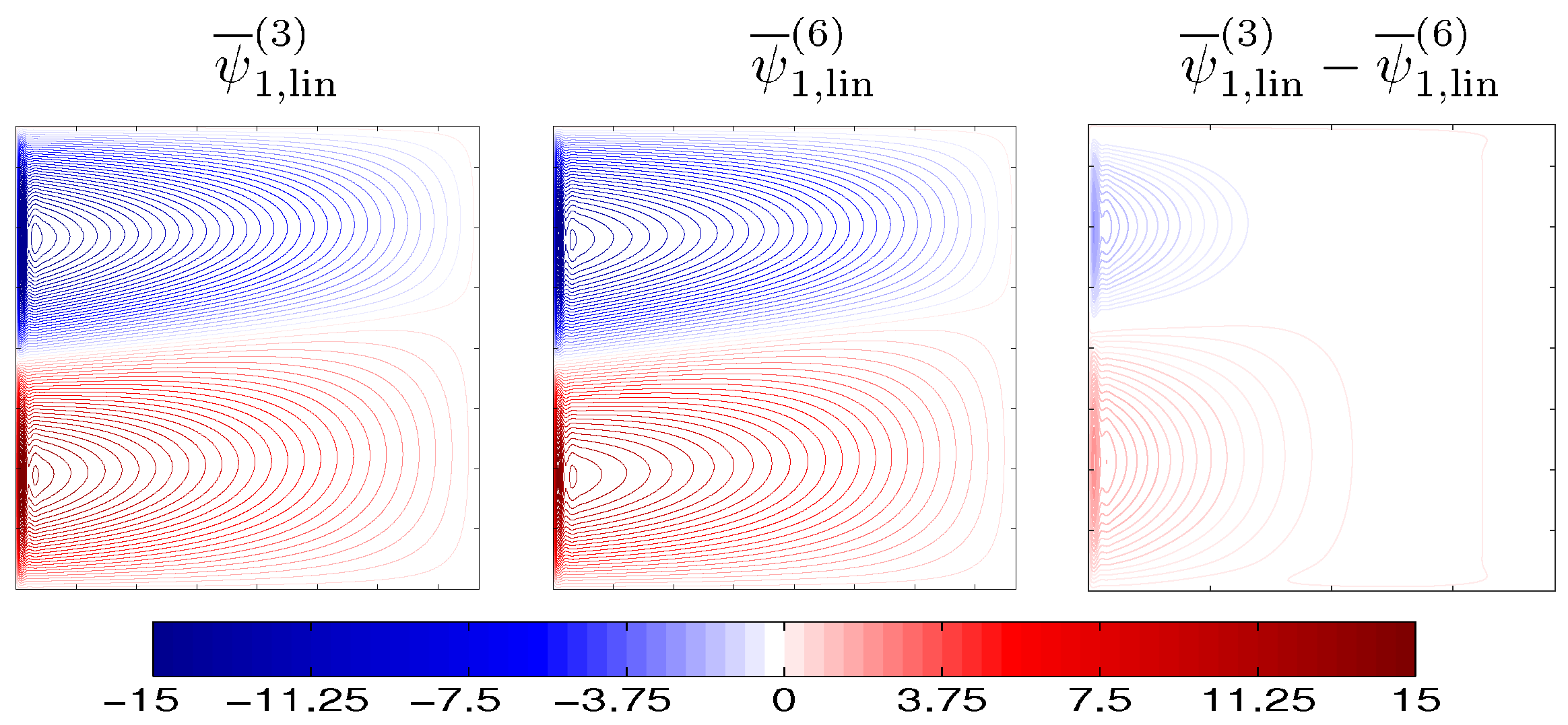
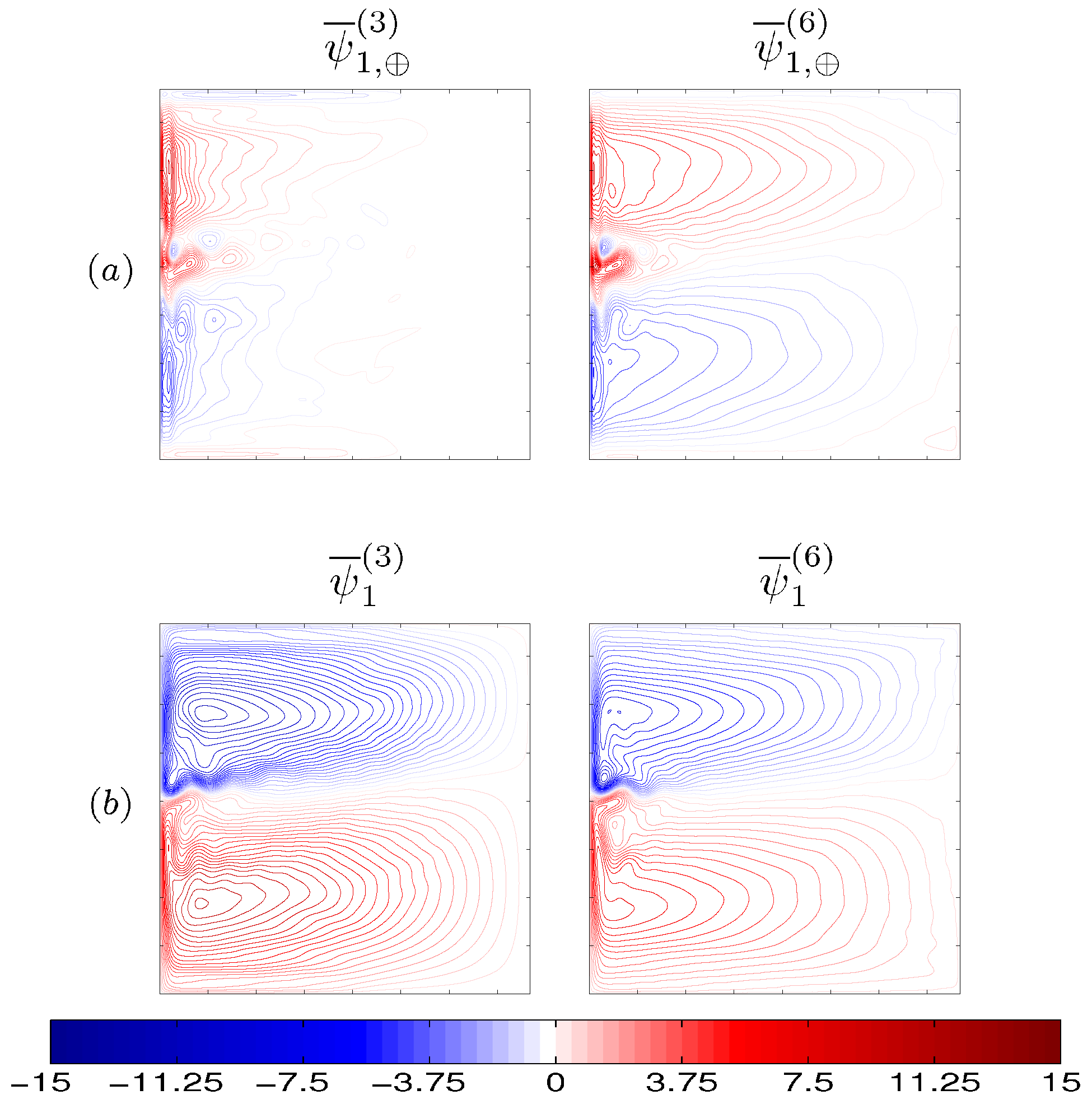
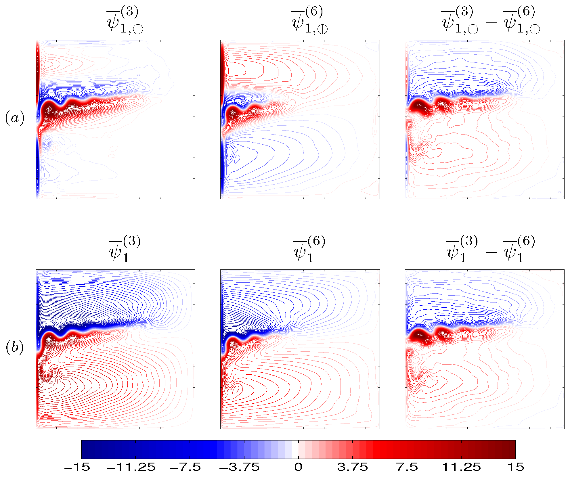
Before passing on to the discussion of the results, it is helpful to decompose the flow into the linear part (i.e., linear-dynamics time-mean response) the time-mean eddy-induced nonlinear anomalies, denoted by the subscript “lin” and “⊕”, respectively, and the transient (primed) fluctuations:
ψ = ψ ¯ lin + ψ ¯ + ψ , q = q ¯ lin + q ¯ + q .
In order to check how eddies affect the eastward jet length L p we excluded the linear parts ψ ¯ 1 , lin (the numerical solution of the governing equations linearized around the state of rest and computed with the CABARET method) of the 3L and 6L models, which are essentially the same ( δ ( ψ ¯ 1 , lin ( 3 ) , ψ ¯ 1 , lin ( 6 ) ) = 0 . 07 , Figure 9), and focused on the analysis of the nonlinear eddy-induced anomalies ψ ¯ 1 , (the difference between the fully nonlinear eddy-induced solution ψ ¯ 1 and its linear part ψ ¯ 1 , lin ), for which δ is much larger, i.e., δ ( ψ ¯ 1 , ( 3 ) , ψ ¯ 1 , ( 6 ) ) = 0 . 91 (
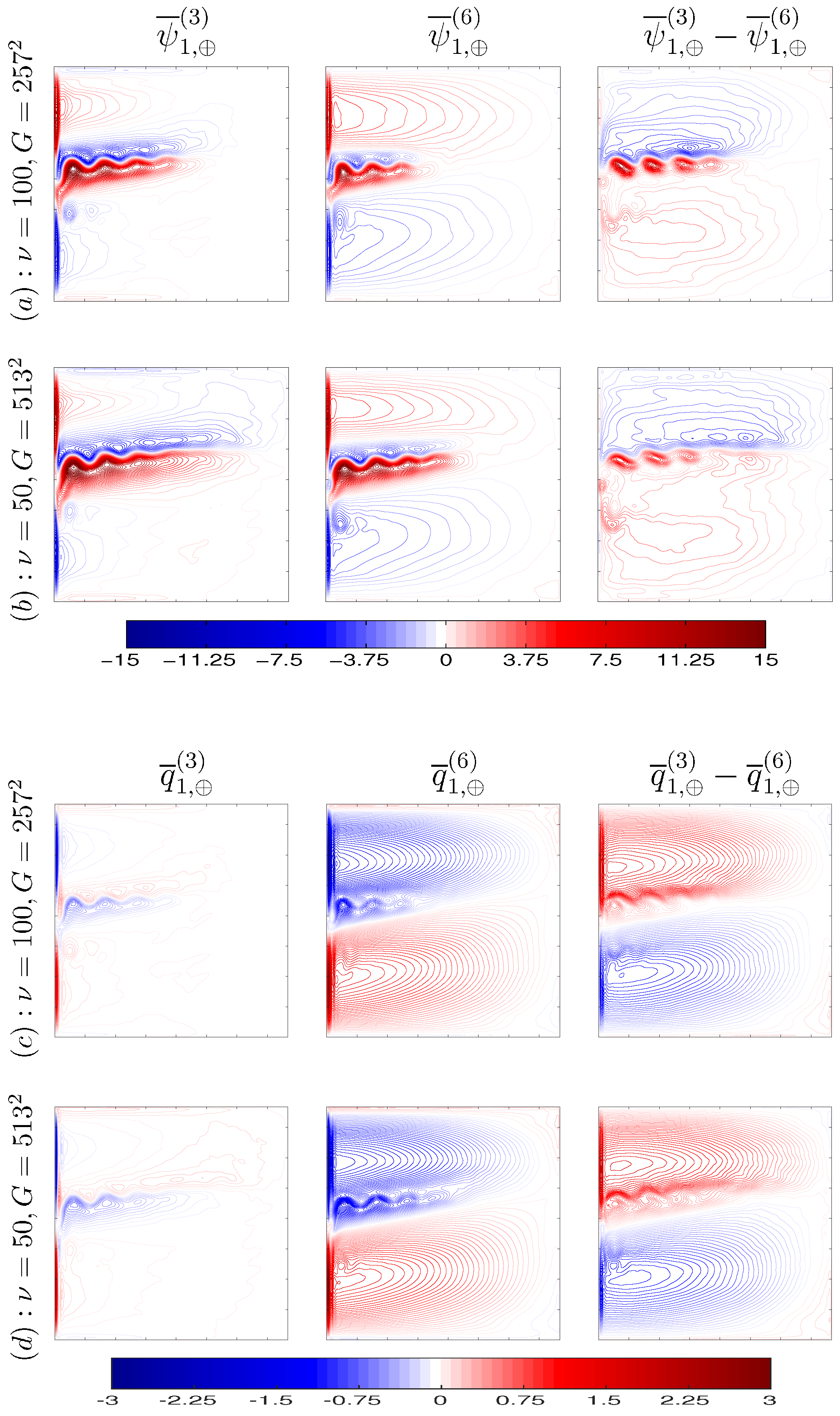
Figure 10a). We found that the difference between the nonlinear components of the 3L and 6L solutions is basin-wide, but with the maximum concentrated mostly around the eastward jet (Figure 10a). To check that this behavior persists with increasing nonlinearity, we carried out another series of experiments with lower ν = 50 m 2 · s 1 and obtained similar difference δ ( ψ ¯ 1 , ( 3 ) , ψ ¯ 1 , ( 6 ) ) = 0 . 91 , also mostly localized around the eastward jet (Figure 10b).
As can be seen in Figure 10, the eddy-induced anomalies are characterized by the opposite-sign PV anomalies embedded in the gyres and slowing them down. We call these flow features “Counter-rotating Gyre Anomalies” (CGAs). The CGAs and their roles in ocean dynamics have never been recognized and analysed in the past, probably, because these flow features are masked by the powerful gyres, hence, they are studied here for the first time. Since CGAs weaken the gyres, which constitute the main pool of energy available to the eddies, it is reasonable to assume that they also inhibit the eddy-driven eastward jet. Can suppression of the CGAs strengthen the gyres and, by feeding more energetic eddies, elongate the eastward jet and enhance its adjacent recirculation zones? This hypothesis, motivated by the fact that weaker gyres (e.g., due to weaker wind forcing) tend to support weaker eastward jet, can be verified by switching the CGAs off with an extra compensating forcing that needs to be found.
Substitution of (8) into (1) and the subsequent time averaging lead to the time-mean balance
J ψ ¯ i , lin + ψ ¯ i , + ψ i , q ¯ i , lin + q ¯ i , + q i + β y ¯ = δ 1 i F ¯ w + D ¯ lin + D ¯ , 1 i N ,
with D = δ i N μ Δ ψ i + ν Δ 2 ψ i .
On the other hand, the linearization of (1) and its time averaging yield
J ψ ¯ i , lin , β y = δ 1 i F ¯ w + D ¯ lin , 1 i N ,
which being substituted into (9) gives
J ψ ¯ i , , β y + J ψ ¯ i , lin , q ¯ i , lin + J ψ ¯ i , , q ¯ i , lin + J ψ ¯ i , q ¯ i , + J ψ i , q i ¯ = D ¯ , 1 i N .
By analyzing the terms in (11) we found that the CGAs are induced by χ ¯ (i.e., by the term J ψ i , q i ¯ ), which is balanced (in the neighborhood of the CGAs) by the term J ψ ¯ i , , β y (the advection of planetary vorticity by the time-mean eddy-induced flow anomaly). The other terms in (11) have negligible effects on the CGAs. Thus, if F χ ¯ i = χ ¯ i is added to the right hand side of (1), it should induce the circulation anomalies in the direction opposite to the CGAs. Full dynamical interpretation of this advection term, as well as explanation of the nonlinear mechanism responsible for it, is beyond the scope of this paper. Enhancing the CGAs weakens the eastward jet in both 3L and 6L solutions (Figure 11a,b), that is consistent with our hypothesis. When we suppress the CGAs, the eastward jet strengthens only in 3L case, but remains nearly the same in the 6L solution (Figure 12).
In the presence of higher baroclinic modes (6L case) the CGAs become wider and stronger and this happens along with the weakening of the eastward jet. Explaining this CGAs amplification is beyond the scope of this paper, but we hypothesize that the weaker 6L eastward jet implies a weaker barrier to cross-gyre PV transport by material particles [23]. Hence, more opposite-sign PV penetrates into each gyre from the other gyre. This mechanism can be interpreted as “cooling” of the gyre, and its direct verification requires analysis of PV on Lagrangian trajectories.
Summarizing the results, we found that F χ ¯ inhibits the eastward jet by creating zonally elongated anticyclonic/cyclonic CGAs in the subpolar/subtropical gyre. However, this effect is moderate, and the jet is still more actively maintained by the eddy backscatter mechanism.
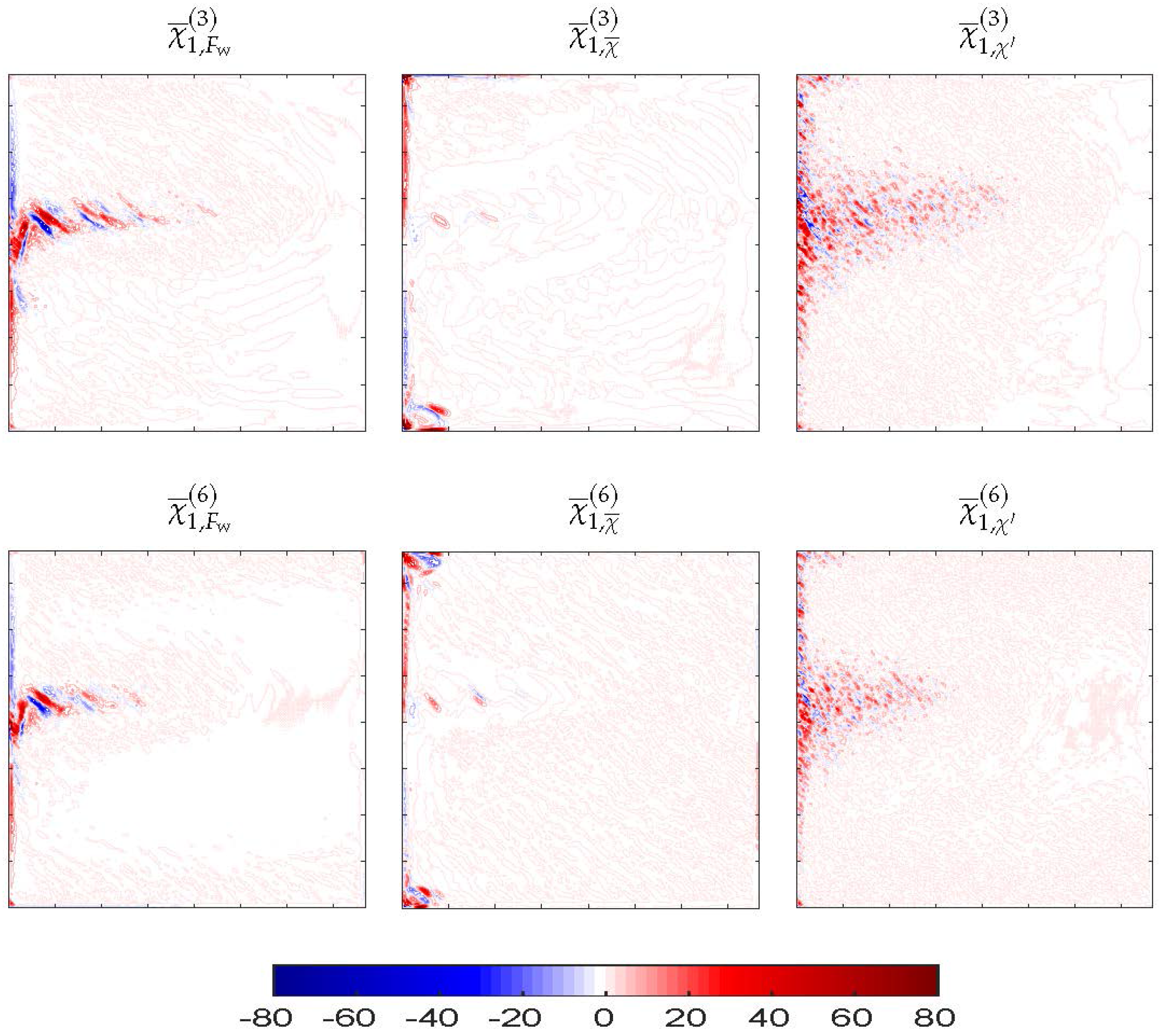
It is useful to compare how the time-mean eddy forcing χ ¯ depends on different forcings used in our study (Figure 13). In the solution driven by the constant wind forcing F w , χ ¯ is strong and mostly concentrated in the eastward jet and its recirculation zones, while in case of the solution forced with the time-mean component of eddy-forcing, χ ¯ is located along the western boundary. In the latter case, the eddy forcing is weak, since it is significantly inhibited by the CGAs (Figure 3a). On the contrary, the 3L solution forced with χ shows a 30 % stronger χ ¯ , which populates smaller scales. However, in the 6L case, χ ¯ is 30 % weaker (Figure 3) thus indicating that the CGAs are strong in both χ ¯ and χ . Thus one can explain the elongation or shortening of the eastward jet by the competition between the CGAs and eddy backscatter: if the CGAs overcome the eddy backscatter then the jet shortens, if the eddy backscatter is stronger than the CGAs then the jet elongates.

4. Conclusions

The goal of this study was to upgrade our knowledge of the eddy/mean interactions in the oceanic double gyres. More specifically, we focused on how eddies affect the eastward jet extension of the western boundary currents and the interior gyres. The novelty of this work is a systematic study of the corresponding nonlinear eddy effects and mechanisms in the idealized eddy-resolving model as a function of increasing vertical resolution and decreasing eddy viscosity.
By systematic analyses of three- (3L) and six-layer (6L) solutions of the multi-layer quasi-geostrophic (QG) model of the wind-driven ocean gyres, we arrived at the conclusion that the eddies have two mutually competing effects on the eastward jet and its adjacent recirculation zones: supporting (or catalyzing) effect, through the eddy backscatter; and inhibiting effect, through induction of the Counter-rotating Gyre Anomalies (CGAs, or the negative/positive PV anomaly in the subpolar/subtropical gyre with circulation opposite to the gyre). All 3L/6L differences are due to the nonlinear eddy effects, since the linear solutions are nearly the same.
We found that the eastward jet and its adjacent recirculation zones are maintained mostly by the rectification of the transient eddy forcing (the eddy PV flux divergence), although the time-mean eddy forcing also supports the jet. In the 3L and 6L cases the fluctuating component of the eddy forcing has the same structure but different amplitude, which is the key aspect setting the difference between the 3L and 6L solutions. The difference in amplitudes is explained by the following. In the absence of high baroclinic modes, the energy input from the wind is more efficiently focused onto the lower modes, therefore, the eddy backscatter is stronger and dominated by the barotropic and first baroclinic modes. However, the higher baroclinic modes still play an important role by transferring energy to the lower modes. This transfer acts locally, directly into the most active eddy backscatter region around the eastward jet; although the modal energetics are studied in a companion paper, we find it appropriate to remark on this result here. This mechanism is partly compensated by the competing effect: in the presence of higher baroclinic modes, the CGAs become stronger and, thus, further weaken the eastward jet. The overall effect of the high baroclinic modes upon the eastward jet (not shown here) is such that higher than the fifth baroclinic modes play negligible roles, hence, six isopycnal layers should be enough to resolve the important eddy-mean interactions in the ocean gyres. Our results also suggest future focus on the eddy backscatter and CGAs in more realistic primitive-equation models of the gyres. Another direction of future research would be to try to explain the CGAs within the framework of the PV homogenization theory developed in [24].

Acknowledgments

The authors are thankful to the Natural Environment Research Council for the support of this work through the grant NE/J006602/1 and the use of ARCHER (the UK National Supercomputing Service). We express our gratitude to Simon Burbidge and Matt Harvey for their help with Imperial College London cluster, as well as to Andrew Thomas for his help with managing and maintaining the data storage.

Author Contributions

Igor Shevchenko performed the simulations and analyzed the data, Igor Shevchenko and Pavel Berloff wrote the paper.

Conflicts of Interest

The authors declare no conflict of interest.

References

  1. Gula, J.; Molemaker, M.J.; McWilliams, J.C. Gulf Stream dynamics along the Southeastern U.S. Seaboard. J. Phys. Oceanogr. 2015, 45, 690–715. [Google Scholar] [CrossRef]
  2. Marsh, R.A.; de Cuevas, B.; Coward, A.C.; Jacquin, J.; Hirschi, J.J.-M.; Aksenov, Y.; Nurser, A.J.G.; Josey, S.A. Recent changes in the North Atlantic circulation simulated with eddy-permitting and eddy-resolving ocean models. Ocean Model. 2009, 28, 226–239. [Google Scholar] [CrossRef]
  3. Treguier, A.M.; Deshayes, J.; Le Sommer, J.; Lique, C.; Madec, G.; Penduff, T.; Molines, J.-M.; Barnier, B.; Bourdalle-Badie, R.; Talandier, C. Meridional transport of salt in the global ocean from an eddy-resolving model. Ocean Sci. 2014, 10, 243–255. [Google Scholar] [CrossRef] [Green Version]
  4. Berloff, P. On dynamically consistent eddy fluxes. Dyn. Atmos. Ocean 2005, 38, 123–146. [Google Scholar] [CrossRef]
  5. McWilliams, J.C. The Nature and Consequences of Oceanic Eddies. In Ocean Modeling in an Eddying Regime; Wiley: Hoboken, NJ, USA, 2008; Volume 177. [Google Scholar]
  6. Dijkstra, H.; Ghil, M. Low-frequency variability of the large-scale ocean circulation: A dynamical systems approach. Rev. Geophys. 2005, 43, 1–38. [Google Scholar] [CrossRef]
  7. Nadiga, B.; Luce, B. Global bifurcation of Shilnikov type in a double-gyre ocean model. J. Phys. Oceanogr. 2001, 31, 2669–2690. [Google Scholar] [CrossRef]
  8. Sapsis, T.; Dijkstra, H. Interaction of Additive Noise and Nonlinear Dynamics in the Double-Gyre Wind-Driven Ocean Circulation. J. Phys. Oceanogr. 2013, 43, 366–381. [Google Scholar] [CrossRef]
  9. Simonnet, E.; Ghil, M.; Dijkstra, H. Homoclinic bifurcations in the quasi-geostrophic double-gyre circulation. J. Mar. Res. 2005, 63, 931–956. [Google Scholar] [CrossRef]
  10. Hogg, A.; Dewar, W.; Berloff, P.; Kravtsov, S.; Hutchinson, D. The effects of mesoscale ocean-atmosphere coupling on the large-scale ocean circulation. J. Clim. 2009, 22, 4066–4082. [Google Scholar] [CrossRef]
  11. Barnier, B.; Le Provost, C.; Hua, B. On the Catalytic Role of High Baroclinic Modes in Eddy-driven Large-Scale Circulations. J. Phys. Oceanogr. 1991, 21, 976–997. [Google Scholar] [CrossRef]
  12. Smith, K.; Vallis, G. The Scales and Equilibration of Midocean Eddies: Freely Evolving Flow. J. Phys. Oceanogr. 2001, 31, 554–571. [Google Scholar] [CrossRef]
  13. Smith, K.; Vallis, G. The Scales and Equilibration of Midocean Eddies: Forced-Dissipative Flow. J. Phys. Oceanogr. 2002, 32, 1699–1720. [Google Scholar] [CrossRef]
  14. Shevchenko, I.; Berloff, P. Multi-layer quasi-geostrophic ocean dynamics in eddy-resolving regimes. Ocean Model. 2015, 94, 1–14. [Google Scholar] [CrossRef]
  15. Kirtman, B.; Bitz, C.; Bryan, F.; Collins, W.; Dennis, J.; Hearn, N.; Kinter, J., III; Loft, R.; Rousset, C.; Siqueira, L.; et al. Impact of ocean model resolution on CCSM climate simulations. Clim. Dyn. 2012, 39, 1303–1328. [Google Scholar] [CrossRef]
  16. Pedlosky, J. Geophysical Fluid Dynamics; Springer-Verlag: New York, NY, USA, 1987. [Google Scholar]
  17. Vallis, G.K. Atmospheric and Oceanic Fluid Dynamics: Fundamentals and Large-Scale Circulation; Cambridge University Press: Cambridge, UK, 2006. [Google Scholar]
  18. McWilliams, J.C. A note on a consistent quasigeostrophic model in a multiply connected domain. Dyn. Atmos. Ocean 1977, 1, 427–441. [Google Scholar] [CrossRef]
  19. Karabasov, S.A.; Berloff, P.S.; Goloviznin, V.M. CABARET in the ocean gyres. Ocean Model. 2009, 30, 155–168. [Google Scholar] [CrossRef]
  20. Nadiga, B. Orientation of eddy fluxes in geostrophic turbulence. Philos. Trans. R. Soc. A 2008, 366, 2489–2508. [Google Scholar] [CrossRef] [PubMed]
  21. Berloff, P. Dynamically consistent parameterization of mesoscale eddies. Part II: Eddy fluxes and diffusivity from transient impulses. Fluids 2016, 1, 1–22. [Google Scholar] [CrossRef]
  22. Berloff, P. On rectification of randomly forced flows. J. Mar. Res. 2005, 63, 497–527. [Google Scholar] [CrossRef]
  23. Berloff, P.; Hogg, A.; Dewar, W. The Turbulent Oscillator: A mechanism of Low-Frequency Variability of the Wind-Driven Ocean Gyres. J. Phys. Oceanogr. 2007, 37, 2363–2386. [Google Scholar] [CrossRef]
  24. Rhines, P.; Young, W. A theory of the wind-driven circulation. I. Mid-ocean gyres. J. Mar. Res. 1982, 40, 559–596. [Google Scholar]
  25. Young, W.; Rhines, P. A theory of the wind-driven circulation. II. Gyre with western boundary layers. J. Mar. Res. 1982, 40, 849–872. [Google Scholar]
Figure 1. A sequence of time-mean solutions for decreasing eddy viscosity ν and the constant wind forcing F w . The time-mean transport velocity streamfunction ψ ¯ 1 for different models, grids G and viscosities ν ( m 2 · s 1 ) ; contour interval is 0.5 Sv. Note that L p ( 3 ) > L p ( 6 ) , but L p ( 6 ) L p ( 12 ) for ν = { 50 , 100 } m 2 · s 1 .
Fluids 01 00028 g001
Figure 2. Vertical structure of the potential vorticity q for the 3L, 6L, and 12L models at ν = 100 m 2 · s 1 and G = 257 2 ; contour interval is 0 . 05 Sv normalized by the Coriolis parameter f 0 = 0 . 83 × 10 4 s 1 . Note that the upper layer is the most active, and activity rapidly decreases with depth. To compare the 3L, 6L and 12L solutions, we projected 6L and 12L solutions onto the 3 layers.
Fluids 01 00028 g002
Figure 3. Flow response to the main eddy forcing components χ ¯ (a) and χ (b) (used as forcing) in no-wind case ( F w = 0 ); contour interval is 0.5 Sv.
Fluids 01 00028 g003
Figure 4. The 3L and 6L model response to the forcing P 6 3 [ χ ¯ ] and P 3 6 [ χ ¯ ] (a); P 6 3 [ χ ] and P 3 6 [ χ ] (b) in no-wind case ( F w = 0 ); contour interval is 0.5 Sv.
Fluids 01 00028 g004
Figure 5. The nondimensional standard deviation of the eddy forcing fluctuating component σ ( χ ) for (a) 3L and (b) 6L solutions.
Fluids 01 00028 g005
Figure 6. The 3L and 6L model response to the force χ ^ ( 3 ) (left) and χ ^ ( 6 ) (right) in no-wind case ( F w = 0 ); contour interval is 0.5 Sv.
Fluids 01 00028 g006
Figure 7. The layerwise response of the 3L model to the selected-mode forcing Θ m 1 [ χ ^ ˜ ( 3 ) ] , m = 0 , 1 , 2 ; contour interval is 0.5 Sv. Note that the flow response is gradually decreasing with increasing m.
Fluids 01 00028 g007
Figure 8. The layerwise response of the 6L model to the selected-mode forcing Θ m 1 [ χ ^ ˜ ( 6 ) ] , m = 0 , 1 , 2 ; contour interval is 0.5 Sv. Shown is only the response to the first three modes, since the higher modes induce a much weaker feedback.
Fluids 01 00028 g008
Figure 9. The linear part of the time-mean transport velocity streamfunction: ψ ¯ 1 , lin ( 3 ) (left); ψ ¯ 1 , lin ( 6 ) (middle); and ψ ¯ 1 , lin ( 3 ) ψ ¯ 1 , lin ( 6 ) (right) for ν = 100 m 2 · s 1 ; contour interval (CI) is 0.5 Sv; δ ( ψ ¯ 1 , lin ( 3 ) , ψ ¯ 1 , lin ( 6 ) ) = 0 . 07 . Note that CI=0.1 Sv in the right figure.
Fluids 01 00028 g009
Figure 10. Eddy-induced flow anomaly. The upper figure: The time-mean transport velocity streamfunction: ψ ¯ 1 , ( 3 ) (left column), ψ ¯ 1 , ( 6 ) (middle column), and ψ ¯ 1 , ( 3 ) ψ ¯ 1 , ( 6 ) (right column) at (a) ν = 100 m 2 · s 1 and (b) ν = 50 m 2 · s 1 ; contour interval is 0.5 Sv; δ ( ψ ¯ 1 , ( 3 ) , ψ ¯ 1 , ( 6 ) ) = 0 . 91 for ν = { 50 , 100 } m 2 · s 1 . The lower figure: The time-mean PV anomaly: q ¯ 1 , ( 3 ) (left column), q ¯ 1 , ( 6 ) (middle column), and q ¯ 1 , ( 3 ) q ¯ 1 , ( 6 ) (right column) at (c) ν = 100 m 2 · s 1 and (d) ν = 50 m 2 · s 1 ; contour interval is 0 . 05 Sv normalized by the Coriolis parameter f 0 = 0 . 83 × 10 4 s 1 .
Fluids 01 00028 g010
Figure 11. The 3L and 6L model response to the forcing F χ ¯ in terms of the time-mean transport velocity streamfunction ψ ¯ 1 , (a) and ψ ¯ 1 (b) at ν = 100 m 2 · s 1 ; contour interval is 0.5 Sv; δ ( ψ ¯ 1 , ( 3 ) , ψ ¯ 1 , ( 6 ) ) = 0 . 64 and δ ( ψ ¯ 1 ( 3 ) , ψ ¯ 1 ( 6 ) ) = 0 . 48 .
Fluids 01 00028 g011
Figure 12. The 3L and 6L model response to the forcing F χ ¯ in terms of the time-mean transport velocity streamfunction ψ ¯ 1 , (a) and ψ ¯ 1 (b), and their differences at ν = 100 m 2 · s 1 ; contour interval is 0.5 Sv; δ ( ψ ¯ 1 , ( 3 ) , ψ ¯ 1 , ( 6 ) ) = 1 . 12 and δ ( ψ ¯ 1 ( 3 ) , ψ ¯ 1 ( 6 ) ) = 0 . 68 .
Fluids 01 00028 g012
Figure 13. Upper-layer time-mean eddy forcing χ ¯ for 3L and 6L solutions driven by the constant wind forcing F w , the time-mean χ ¯ and fluctuating χ components of eddy forcing, respectively; contour interval is 5 . 0 s 2 .
Fluids 01 00028 g013
Table 1. The depths of isopycnal layers (in (m)) for 3L, 6L and 12L models.
Layers H 1 H 2 H 3 H 4 H 5 H 6 H 7 H 8 H 9 H 10 H 11 H 12
30.250.753.0
60.250.250.250.251.002.0
120.1250.1250.150.150.150.150.150.20.30.51.01.0
Table 2. The Rossby deformation radii (in (km)) for 3L, 6L and 12L models.
Layers R d 1 R d 2 R d 3 R d 4 R d 5 R d 6 R d 7 R d 8 R d 9 R d 10 R d 11
340.023.0
640.016.011.69.87.8
1240.015.710.78.26.66.25.34.63.93.63.2
Table 3. Large-scale flow properties. The time-mean eastward jet penetration length L p ( km ) , the total volume transport Q ( Sv ) , and the relative errors δ for different values of the eddy-viscosity ν ( m 2 · s 1 ) in the 3L, 6L and 12L solutions.
ν L p ( 3 ) L p ( 6 ) L p ( 12 ) Q ( 3 ) Q ( 6 ) Q ( 12 ) δ ( ψ ¯ 1 ( 3 ) , ψ ¯ 1 ( 6 ) ) δ ( ψ ¯ 1 ( 6 ) , ψ ¯ 1 ( 12 ) )
10023701740175510390910.610.05
502865236023021231191310.570.05
Table 4. Transient eddy forcing. The basin-average integral of the standard deviation of the fluctuating component of the eddy forcing χ .
Layer I Ω ( σ ( χ ( 3 ) ) ) I Ω ( σ ( χ ( 6 ) ) )
118.8515.55
22.555.77
30.782.43
41.19
50.54
60.52
Table 5. The efficiency of the modes E = Q ( ψ ¯ F ( i ) ) Q ( ψ ¯ ( i ) ) for the selected-mode forcing F = Θ m 1 [ χ ^ ˜ ] in the 3L and 6L solutions.
m-th Mode E ( 3 ) E ( 6 )
00.580.80
10.520.64
20.310.08
30.10
40.04
50.05

