
Scalar Flux Kinematics


1
Department of Physical Oceanography, Mail Stop 21, 266 Woods Hole Rd., Woods Hole Oceanographic Institution, Woods Hole, MA 02543, USA
2
Department of Atmospheric and Oceanic Sciences, University of California and Los Angeles, Los Angeles, CA 90095-1565, USA
*
Author to whom correspondence should be addressed.
Fluids 2016, 1(3), 27; https://doi.org/10.3390/fluids1030027
Submission received: 16 May 2016
/
Revised: 15 July 2016
/
Accepted: 18 July 2016
/
Published: 25 August 2016
(This article belongs to the Collection Geophysical Fluid Dynamics)
Abstract
:The first portion of this paper contains an overview of recent progress in the development of dynamical-systems-based methods for the computation of Lagrangian transport processes in physical oceanography. We review the considerable progress made in the computation and interpretation of key material features such as eddy boundaries, and stable and unstable manifolds (or their finite-time approximations). Modern challenges to the Lagrangian approach include the need to deal with the complexity of the ocean submesoscale and the difficulty in computing fluxes of properties other than volume. We suggest a new approach that reduces complexity through time filtering and that directly addresses non-material, residual scalar fluxes. The approach is “semi-Lagrangian” insofar as it contemplates trajectories of a velocity field related to a residual scalar flux, usually not the fluid velocity. Two examples are explored, the first coming from a canonical example of viscous adjustment along a flat plate and the second from a numerical simulation of a turbulent Antarctic Circumpolar Current in an idealized geometry. Each example concentrates on the transport of dynamically relevant scalars, and the second illustrates how substantial material exchange across a baroclinically unstable jet coexists with zero residual buoyancy flux.
1. Introduction
Kinematic analysis of geophysically relevant fluid flows has in the past several decades been elevated by dynamical-systems-based methods that enable identification of key material contours or surfaces central to transport and stirring processes. In some cases, the contours are touted as barriers to material transport, and although any material contour is by definition a barrier, there are some that are particularly significant. For example, a long-lived, coherent eddy is often surrounded by a closed material contour that undergoes minimal material stretching [1,2,3]. The contour does not undergo filamentation or roll-up and therefore can be used to objectively define a boundary that contains fluid that is trapped by the eddy and perhaps transported over large distances [4]. Another set of significant objects consists of the stable and unstable (attracting and repelling) material manifolds of hyperbolic trajectories. Material manifolds provide a framework for lobe dynamics, perhaps the most beautiful method of Lagrangian transport analysis. Apparently first applied to the problem of fluid transport by [5,6] this approach provides for the visualization and quantification of material transport between qualitatively different regions of a time-varying flow field.
We will present an overview of contributions made roughly over the past two decades, focusing on those that have impacted the field of physical oceanography. The review is not intended to be exhaustive or mathematically rigorous, and the reader should consult the references, particularly [7,8], for more formal treatments. The intent of the review is to emphasize accomplishments and limitations, and the latter will lead us to consider an alternative approach that combines elements of Lagrangian analysis with a desire to comprehend property fluxes other than fluid material.
Perhaps the most enduring example of Lagrangian transport analysis in physical oceanography is the computation of exchange between two counter-rotating gyres, depicted in Figure 1a as the cyclonic and anticyclonic members of a dipole or double-gyre system. In a steady configuration, two hyperbolic stagnation points S1 and S2 are connected by a streamline that separates the two members. If a moderately weak, time-periodic disturbance is added to the velocity field, S1 and S2 will survive in the form of moving hyperbolic trajectories H1 and H2, for which the surrounding flow is, on average, convergent in one direction and divergent in another (Figure 1b). For example, the flow surrounding H1 will tend to be convergent, on average, in the along-shore direction and divergent in the offshore direction. The positions of H1 and H2 will generally vary with time, but if the disturbance is not too large, both points will linger in the neighborhood of the original stagnations points. If one were to continuously introduce dye into the vicinity of H1, it would be attracted to H1 in the along-shore direction, but would be repelled in the offshore direction forming a long streak. This streak would be an approximation of the unstable manifold (also called the “outgoing” manifold) consisting of material that diverges from H1 (approaches H1 in backward time). The unstable manifold of H1 is depicted by red contour in Figure 1b. Similarly, stable and unstable manifolds can be defined for H2 as material, time-dependent curves consisting of fluid elements that approach H2 asymptotically in forward or backward time. All of the manifolds evolve over time and Figure 1b is just a snap shot, but if the time-dependence is periodic the shapes will recur periodically.
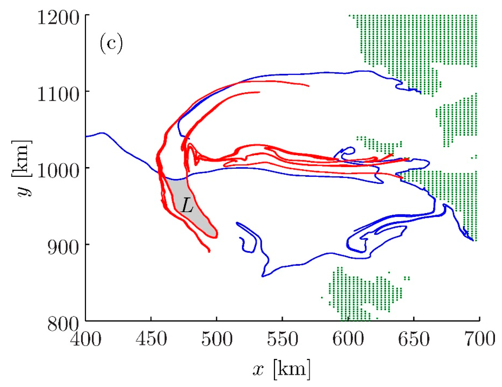
In the steady case (Figure 1a) the unstable manifold of S1 is also a stable manifold of S2 and can be thought of as a boundary separating the cyclonic and anticyclonic members of the dipole. In the unsteady case, these manifolds are distinct, and it is common for the unstable manifold of H1 to intersect the stable manifold of H2. One can identify lobes of fluid L1, L2 whose boundaries consist of segments of the intersecting manifolds. As the flow evolves, the lobe L1 will move from right to left, continuing to be bounded by the same sections of the material curves. If the time dependence is periodic, the shapes of the curves will recur after a single period, and the fluid in L1 will have moved into the space depicted as L2 in the figure. After another period the fluid will have moved to the space occupied by L3 and so on, so there is clearly a transport from the cyclone to the anticyclone. In the same manner, fluid in lobe L−1 evolves into L−2 and so on, defining a transport process from the anticyclone to the cyclone. This mechanism leads to exchange between the two gyres, and the lobes are therefore called turnstile lobes. As implied in Figure 1, the lobes themselves tend to be continuously stretched and folded, so that property gradients within are amplified and irreversible property exchange through diffusion is enhanced. In time-periodic systems, the motion of fluid parcels is often described by a Poincare’ map, in which discrete parcel positions are plotted at the end of each period. In this description, the manifolds in Figure 1b remain frozen, fluid parcels remain on the fixed manifolds as they are mapped from one position to the next, and fluid blobs are mapped from one lobe to another. We prefer to think about the manifolds as time-continuous objects since this picture is relevant to the time aperiodic case, which can be similar in concept and geometry. An example from a numerical simulation of a strongly aperiodic, surface dipole in the Philippine Seas [9] appears in Figure 2.
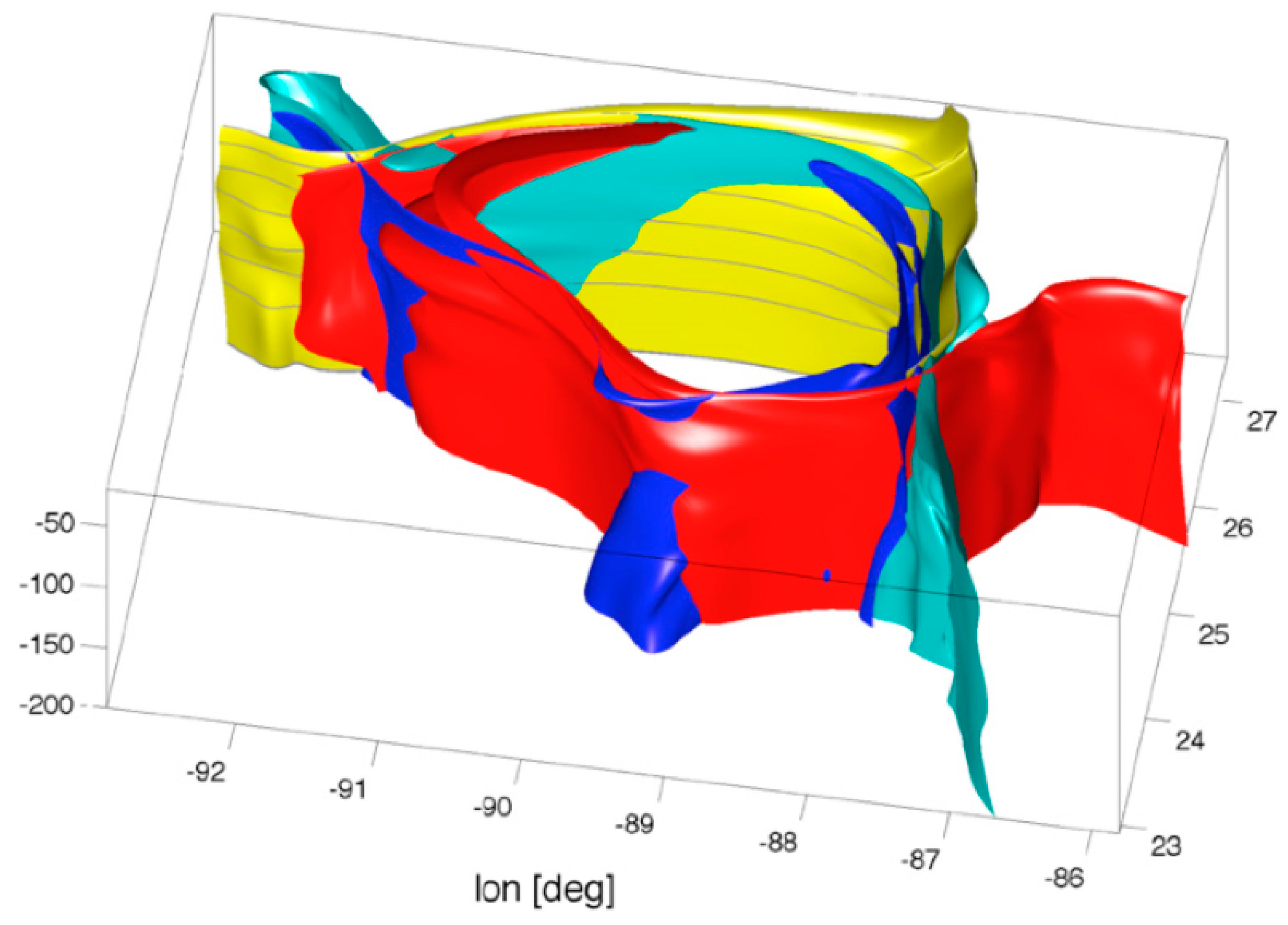
Lobe analysis has been applied to a number of oceanographically relevant flow fields including meandering jets [10], dipoles and counter rotating gyres [11,12,13,14,15], boundary-trapped recirculations [16], and breaking Rossby waves [17]. In most cases the velocity field is assumed to be two-dimensional and divergence free, which limits the zoology of stagnation points to just two types: hyperbolic and elliptic. The analysis has been applied [18] to a three-dimensional model of a Gulf of Mexico Loop Current eddy, but the weakness of the vertical velocity implies that the horizontal velocity field is approximately nondivergent at each depth, enabling the authors to construct a 3D picture by stacking a set of 2D analyses at different horizontal levels. The finite time material manifolds now consist of intersecting surfaces (Figure 3), with finite volume lobes of fluid trapped between. Due to the lengthy analysis involved in making just a single snapshot of the lobes, the authors did not attempt any transport calculations.
When the velocity fields are known only over finite time, or when strong hyperbolicity is limited to a finite time window, objects similar to stable and unstable material manifolds may still be found. As pointed out in [19], persistent hyperbolicity can occur when the Eulerian time scale of the flow is much longer than the Lagrangian time scale. This time scale separation can occur in the so-called chaotic advection regime, when the flow field is dominated by long-lived coherent structures, often in the form of eddies. For example, a concentrated hyperbolic region can form between eddies of like sign and may persist over many eddy winding times (see point “1” in Figure 4). If a passive tracer is introduced in this region, it will experience contraction in one direction and expulsion in another direction, all in analogy to the stable and unstable directions of a hyperbolic trajectory. Thin material streaks of tracer that emanate from the hyperbolic region in the unstable direction in forward time (or in the stable direction in reverse time) exhibit behavior similar to that typical for invariant manifolds. These objects are collectively known as hyperbolic Lagrangian Coherent Structures [20], or LCS, that form a skeleton or template for stirring and transport processes due to their attractive/repelling properties. In this paper, we will use the term “finite-time manifolds” loosely to refer to the hyperbolic-type LCS that serve as finite-time analogs of infinite-time invariant manifolds from classical dynamical systems theory. In addition to finite-time manifolds (hyperbolic LCS), relevant finite-time analogs of infinite-time material objects from dynamical systems theory include closed contours defining the boundaries of coherent eddies (elliptic LCS), which are or analogs of KAM tori, and material barriers defined by minimal Lagrangian shear (parabolic LCS), which are analogs of shearless trajectories (e.g., the central axis of a jet) and can exhibit strong stability under perturbation in certain types of Hamiltonian systems [1]. An example of the latter can be found in [21]. Even when hyperbolic-type LCS can reasonably be defined in finite time, it may or may not be advantageous to perform a lobe analysis. However, the finite-time LCS themselves still yield valuable information as to which regions of the flow field are being most rapidly stirred and whether barriers to chaotic transport exist. An example of success comes from Monterey Bay [22], where the circulation has a strong tidal component. Maps of LCS yield information about how the bay is flushed. Other successful applications include the Adriatic Sea [14], where the circulation is dominated by three coherent gyres, and the Phillipine Sea [9] where the transport of nutrients from Manila Bay into an offshore dipole can be tracked using manifold-type analysis.
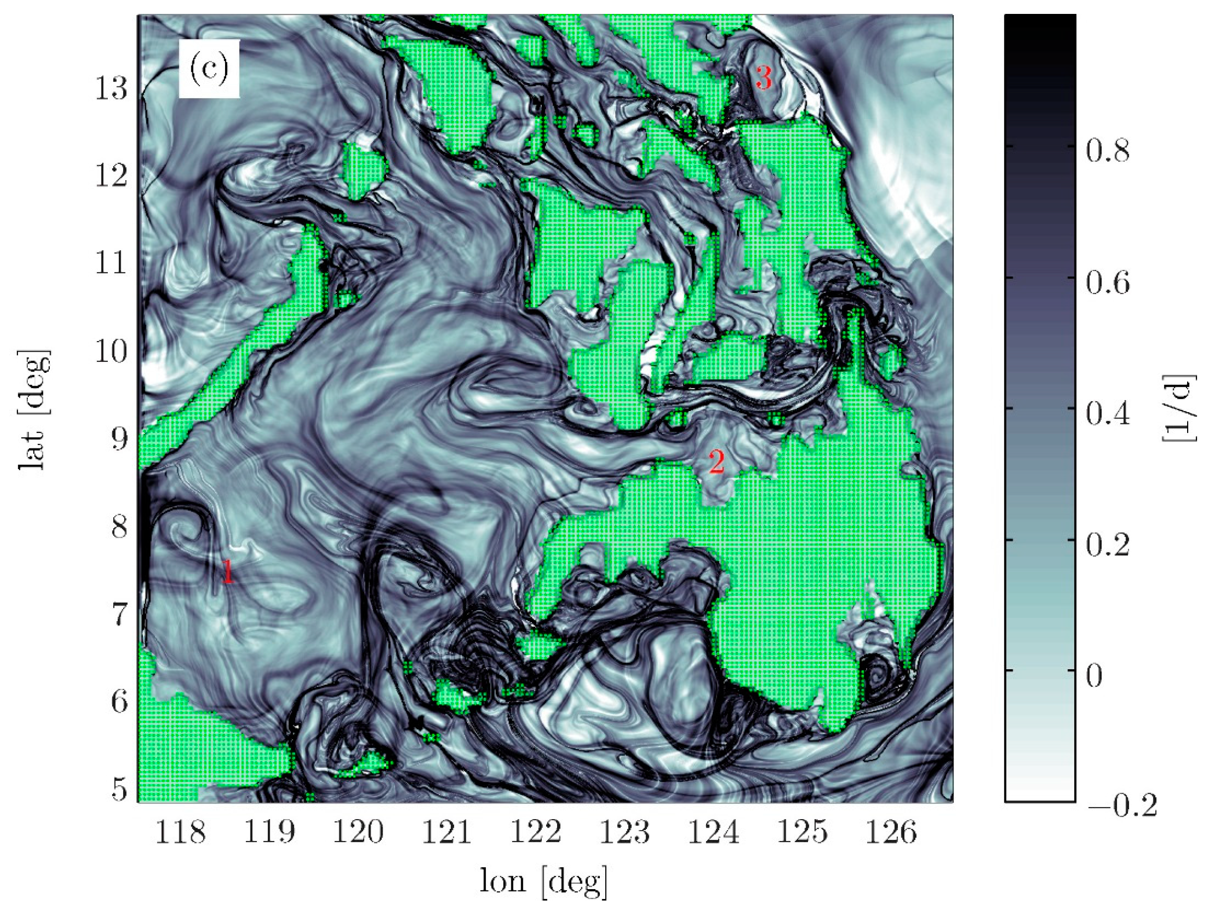
As an example of the type of information that can be gained, consider a plot of 7-day backward and forward, finite-time Lyapunov exponents (FTLEs), computed using a model of the Philippine Seas (Figure 4) and based on the surface velocity field. The ridges of the FTLE fields are often used to approximate finite-time material manifolds [20,23]. (Though regions of strong shear can sometimes result in FTLE ridges that are not associated with hyperbolic-type LCSs, these cases are generally rare in realistic oceanic flows. See [1] for a more rigorous approach to identifying LCS.) Areas that are densely covered by intersecting curves indicate regions of rapid stretching and folding of material whereas regions that are clear tend to be more slowly stirring, isolated and more regular. Examples of the latter include the interiors of “Figure-eight” separatrix formed by two nearby anticyclonic eddies (marked “1”) and two topographically constrained recirculations (marked “2” and “3”). A more recent approach [24] to the identification of mixing zones, based on averages of hyperbolicity along trajectories, has been applied to an oil spill in the Gulf of Mexico.
Much of the current interest in Lagrangian dynamical systems analysis is focused on elliptic LCS, closed material contours that exhibit uniform stretching and that can define the boundaries of various types of vortices. The underlying idea is that a boundary that rolls up and develops filaments would undergo non-uniform stretching. Variational methods for computing these objects have been developed [1,2] and applied to features such as S. Atlantic surface eddies generated in the South African “caldron” [4]. By defining and computing bounding elliptical contours, the authors have identified eddies that can remain coherent over thousands of km (Figure 5). Other Lagrangian approaches for the identification and tracking of coherent eddies include transfer operator methods [25], in which the most coherent sets of trajectories starting from a grid of initial positions are computed. This approach has been successfully used to track 3D Agulhas eddies in numerical simulations [26]. Koopman mode analysis [27,28] also has the potential to identify features that are coherent in a Lagrangian sense. Here, time averages of fixed scalar fields are taken along individual trajectories and clustering algorithms are used to identify those trajectories most similar in terms of Lagrangian averages. Other measures that potentially identify LCS include trajectory arclength [29,30] and other measures of trajectory complexity [30]. There is always debate as to whether objects identified by various methods are material following. If the approach is based on a frame-dependent measure such as Eulerian vorticity, then there is an obligation to demonstrate that the computed object is, in fact, Lagrangian.
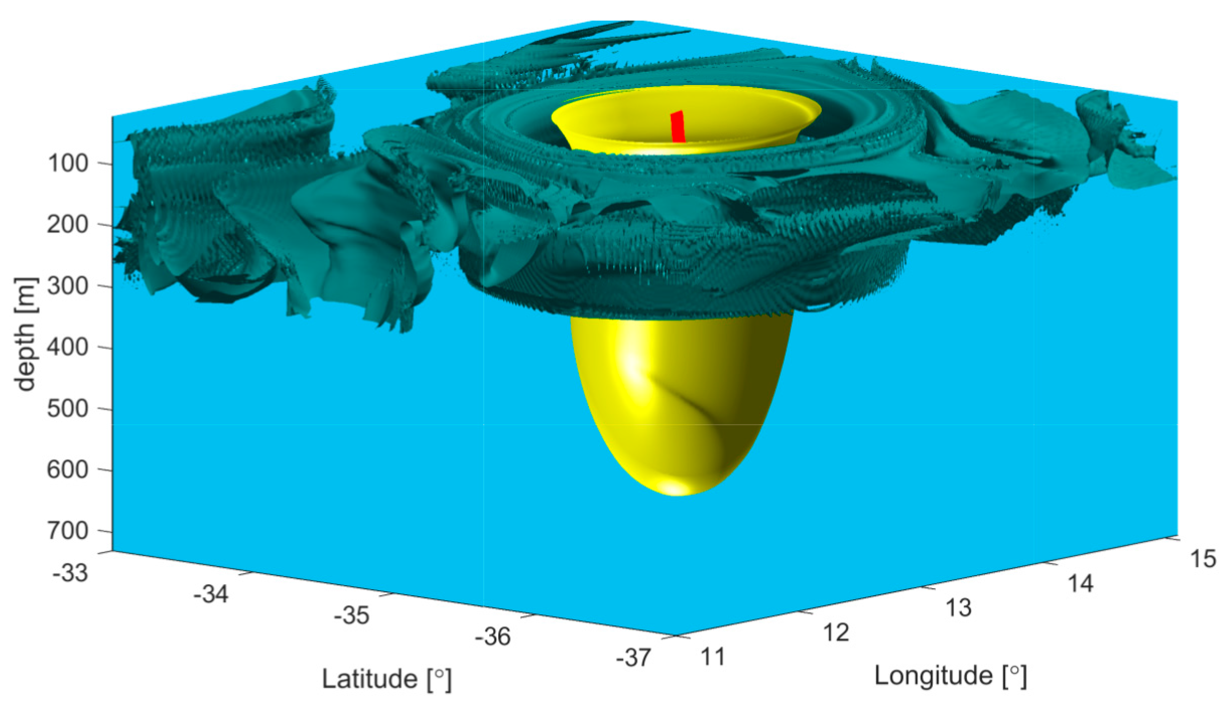
Although elliptic LCS identify coherent structures in the flow field, there is no guarantee that these structure are eddies, at least not in the sense that they are identified with anomalously high vorticity. This has led to a search for boundaries that remain coherent and that are identified by high anomalous Lagrangian-averaged vorticity deviation [15] (and also see [31]). An example of a conical boundary surrounding a surface vortex a 3D simulation of the upper ocean is shown in Figure 6.
Recent attention has been directed towards a better understand of the barriers and chaotic regions of fully 3D flows that have a vertical velocity (w) that is significant in the sense that vertical derivative of w is as large as the horizontal divergence of the horizontal velocity. This is not the case in quasigeostrophic motion, where the divergence of the horizontal velocity is zero to leading order. In this setting the zoology of stagnation points enlarges to include spiral structures [33]. Oceanographically relevant flow fields often involve divergent surface and bottom Ekman layers, sub-mesoscale filaments and fronts, and convection cells. Other studies [34,35] use idealized but dynamically consistent flow fields. A canonical example that has applications in physical oceanography and engineering, and whose Eulerian characteristics have been studied extensively, is the rotating cylinder flow [34]. In one of many possible configurations of this flow (Figure 7a), the circulation in the cylinder is driven by a differential stress distribution at the top surface, and this results in a flow field that has horizontal swirl and vertical overturning, with spiraling trajectories that recirculate on tori. When the axial symmetry of the flow is broken in some manner, some of the tori brake resulting in the formation of chaotic resonant layers, separated by material barriers. These barriers also take the form of tori, as shown by several examples (Figure 7b). Three dimensional ABC flow [15,27] and a kinematic model of neighboring convection cells [36] form the basis for other commonly-considered 3d examples.
Despite considerable theoretical and computational advances in the identification of important material objects, the field of LCS analysis faces a number of limitations in its application to mainstream physical oceanography. One is that the transport calculations, whether they follow from lobe analysis or from the tracking of elliptic contours or surfaces, give only a volume flux (or area flux in 2D), and while this may be of significance, one is typically more interested in the transports of other scalar properties such as heat, salt, momentum, vorticity, energy, contaminants or chemical and biological tracers. If the scalar is approximately conserved following the fluid, then LCS analysis has direct implications for the scalar flux. However oxygen, momentum components, and other dynamical and biological tracers can be highly non-conservative. An attempt was made [16] to confront this challenge in the context of an unstable, boundary trapped gyre in a model of wind-driven, barotropic ocean circulation (Figure 8). At issue are the dynamical mechanisms for driving the circulation in the gyre, which include the wind but also potential vorticity advection into and out of the gyre by eddies. The dynamics can be summarized by writing down the circulation integral for the barotropic flow on a beta plane:
where is the potential vorticity, ζ is the relative vorticity, β is the rate of change of Coriolis parameter with latitude, τ is the surface wind stress, ρ is the (uniform) density, AH is the horizontal eddy viscosity, H is the constant ocean depth, and u is the horizontal velocity. The contour integrals are taken about the boundary of a region R that contains the gyre. The integrals on the right-hand side of Equation (1) measure the advection of potential vorticity across , the tangential component of stress on , and the horizontal frictional stress acting along . The sum of these terms can cause the gyre to spin up or down, as measured by the rate of change of circulation (first term in the left-hand side), and/or cause the mean latitude y of the gyre to increase or decrease (second term in the left-hand side). By constructing a time-dependent boundary using pieces of stable and unstable manifolds, the authors were able to quantify the advection of q into and out of the gyre as a lobe exchange processes. The approach requires that one first computes the manifolds and lobes, then separately calculates the amount of area-integrated q for each lobe entering or leaving the gyre at irregular intervals.
In a more recent attempt [37,38] to calculate scalar property fluxes using lobe analysis, the velocity and scalar tracer fields are partitioned into a time mean and a time-varying perturbation. The boundary across which the tracer transport is computed is chosen as a mean streamline and the flux is associated with “psuedo lobes” formed by a material contour that initially coincides with a mean streamline but that begins to meander back and forth across it as the result of transverse motion. The method is formulated based on perturbation theory and hence requires variations (i.e., perturbations) about the means of the velocity and tracer field to be small. The method can be used as a diagnostic tool for Lagrangian transport and is applied by the authors to the problem of exchange of a passive tracer between two gyres.
The second limitation is that eddy resolving flow fields are often so complex that computation of Lagrangian material transport would require a prohibitively intricate level of bookkeeping. This is evident, for example, in a study of transport between the Atlantic Ocean subtropical and subpolar gyres ([39] and Figure 9). There the intersecting finite-time stable and unstable manifolds (approximated by FTLE ridges) are extremely complex and spring from numerous hyperbolic trajectories. In another study [40], manifold proxies are computed in models of increasing resolution and it is shown that the presence of submesoscale motions causes otherwise smooth LCS to rapidly filament and acquire a level of complexity that would surely undermine the type of mesoscale lobe computations presented in [18]. Of course, these findings are dependent on the model’s representation of submesoscales, a feature that is difficult to validate. In fact, some studies [41,42] have found good agreement between observed surface drifter motion and LCS computed from altimeter-based velocities.
This all begs the question of whether it is possible to develop an approach that retains some of the flavor and intuition afforded by LCS analysis, that yields direct information about fluxes of specific physical properties, and that can somehow avoid bookkeeping difficulties that can arise in intricate flow fields. To accomplish the latter, the method must treat some smoothed version of the flow and yield fluxes that are meaningful. The approach developed below is a possible step in that direction and our purpose here is to describe it and point out some strengths and weaknesses. As with most other types of Lagrangian analysis, it is completely diagnostic and requires that the fluid velocity and tracer fields are known in advance. In the case of a dynamically active tracer such as buoyancy or vorticity, the flux is determined by the velocity and thermodynamic variables (pressure, density, temperature, etc.), all of which are part of the model output. If the tracer is passive, then a separate calculation is required, perhaps with an advection-diffusion equation, in order to establish the tracer fields, with different distributions following from different initial conditions.
2. Results
2.1. Kinematics of a Residual Scalar Flux
Consider a scalar property C that is governed by the conservation law
where S represents all the sources and sinks of C and F represents the flux of C. This form is quite general and, in fact, not unique, for one may have a choice whether to include specific terms in or assign them to S. For our purposes it will be advantageous to include in as many terms as possible. The flux vector F will generally contain contributions from advection by the fluid velocity u and from molecular or sub-grid scale diffusion. As we shall show, it may also contain certain types of forcing. It is not uniquely defined, as one can add to it any non-divergent vector. In many cases, the best choice of F is determined by boundary conditions and/or by the considered formulation of the specific budget or science question that one wishes to address. Further discussion on this point follows below.
Any particular F can be nonuniquely represented as the product of an arbitrary scalar quantity γ(x,t), with the same units as C, and a corresponding velocity u*(x,t), so that u* = F/γ. For a given choice of γ, consider the trajectories x*(t; xo*,to) of the velocity field u*, as determined from
In most of the applications explored later on u* is divergent, however we will assume that u* is sufficiently well behaved that the mapping of the initial condition to its destination at time t is unique and invertible.
Under these conditions, we may then define a volume Vγ(t) enclosed in surface Aγ(t) that is obtained by evolving a surface Aγ(0) of initial conditions forward under Equation (3). Integration of Equation (2) over this volume then yields
where n is the outward normal to Aγ(t) and where Leibnitz’s rule is used in the first step. With the choice , this relation simplifies to
Thus, the total amount of tracer in VC(t) remains conserved if its boundary AC(t) is advected with the velocity and if S (or its integral over VC(t)) is zero. In this sense, the boundary acts as a “barrier” for the tracer in the same way that material contours act as barriers to material transport. However, u* will generally be divergent and may be infinite (as in our first example below) so that finite-time invariant manifolds, hyperbolic and elliptic LCS and the like may not exist in the established sense.
As a simple example, consider the advection/diffusion equation for temperature T of the fluid in the presence of an incompressible fluid velocity u:
The molecular diffusivity κT is considered constant. We have the choice of writing the right hand side as , where , or as , where and . In first case whereas in the second u* = u. The advantage of the fist choice is that a closed volume advected with the velocity u* will conserve total heat.
As a second example illustrating the flexibility one may have in assigning terms normally regarded as sources or sinks to , consider the potential vorticity equation for a single-layer model of wind-driven, homogeneous ocean circulation on a β-plane:
Here is the potential vorticity, ψ is the stream function, is the bottom elevation, τ is the wind stress, r is a bottom drag coefficient and 1/Re is the horizontal eddy viscosity. The nondimensionalization and definition of the other scales can be found in [43]. Equation (7) attributes the rate of change of q to advection of q (second term on the left), vortex stretching due to Ekman pumping (first term on right) and bottom and lateral friction (final two terms). The equation may be rewritten in the form
where
where . Thus, the wind forcing and dissipation terms, normally regarded as belonging to the source and sink term S, may all be absorbed into F. The total amount of potential vorticity carried by a volume advected by the velocity field u* = F/q is thus conserved.
The previous examples illustrate how patches or volumes containing fixed amounts of heat and potential vorticity can be identified and tracked in time. It remains to be seen how useful this construction is in particular problems, but since heat and potential vorticity transport are of fundamental importance in processes such as baroclinic and barotropic instability, wave-mean flow interactions, and general circulation and climate, the prospects are intriguing.
The distribution of a scalar in a turbulent flow can be quite complex, with fine filaments, even if the advecting velocity field is smooth, so u* may be considerably more complex than the fluid velocity field. It then becomes desirable to consider smoothed versions of the velocity and tracer fields. We therefore consider a low-pass filter, taken over a window of length T:
Again, the choice of T is guided by the particular problem at hand. For our purposes, interpretation of the filter is most obvious when the smoothing function s(t′ − t) is unity, for then the filter is just a running average in time of the scalar quantity over T.
The time average of Equation (2) is then,
(using the fact that can be shown to equal ). The foregoing arguments then lead to
where the surface enclosing the volume is now advected by the velocity .
If we partition the velocity and tracer field between the slowly varying mean and departures from it (denoted by a prime), then will commonly take the form but may include other terms as well. Note that the ‘Leonard’ flux terms and arise due to the fact that the “average” terms vary slowly in time [44]. They shrink to zero in the limit T→∞. The full expression describes a residual flux that includes contributions from eddies and from sub-grid diffusion. We will refer to as the residual velocity. It has some similarity to the transformed Eulerian mean (TEM) velocity ([45], Section 7.3) insofar as it measures a residual. It also differs in several respects, one being that the TEM residual is usually composed of an Eulerian mean and an eddy contribution, whereas the flux vector on which may contain diabatic terms such as and even external forcing terms, as shown earlier.
Of course the integral of over does not give the total amount of C in this volume. That amount would be
and Equation (12) must be interpreted accordingly. Even though itself has no temporal average, it may have a finite average over . Nevertheless, one is often most interested in slow changes in the mean value of a tracer and this problem is directly addressed by Equation (12).
We note that traditional LCS analysis is a special case of our approach. The relevant version of the conservation law Equation (2) is the continuity equation
where ρ is the fluid density. The velocity is just the fluid velocity u, usually assumed to be divergence free. Time averaging can be performed as above, resulting in the flux vector for the average mass flux (mean plus eddy), the residual velocity and statement indicating conservation of the total mean mass within a closed volume whose boundary is advected by . (The time-average version has apparently not been used within the LCS community).
Finally, as noted by Prof. George Haller (personal communication), the nonlocal conservation law Equation (12) can be made point wise by shrinking to zero. In this limit , and thus
showing that in the absence of sources and sinks, the change in the mean concentration of the scalar is proportional to the divergence of following the trajectory. The tracer is diluted or concentrated in response to the expansion or contraction of the small volume . The same naturally follows for the non-averaged version.
2.2. Diffusive Transport of Momentum, Vorticity, Energy and Enstrophy in Viscous, Laminar Flow
As a first example, we consider the classical initial-value problem of viscous adjustment of an impulsively started uniform flow u = U and v = 0 in the upper (x, y) plane, bounded by a no-slip, flat plate at y = 0. The x-velocity u is determined entirely by the x-momentum equation, which takes the form of a heat equation:
with initial and boundary conditions
For t > 0 the fluid at y = 0 is immediately brought to a halt and the fluid above the boundary is decelerated towards rest by a viscous layer of increasing thickness. The solution is given by
and the corresponding vorticity and its derivative are
Now suppose that one is interested in the scalar flux of vorticity, which is introduced into the initially irrotational fluid at the boundary at y = 0. The flow is laminar and there is no need to perform the time averaging over turbulent scales, so we seek a conservation law of the form of Equation (2). This is easily obtained through differentiation of Equation (16) with respect to y, resulting in
In terms of Equation (2) we have C = ζ, , and therefore, with
the final step following from substitution of the solution Equation (18).
The trajectories of are obtained from
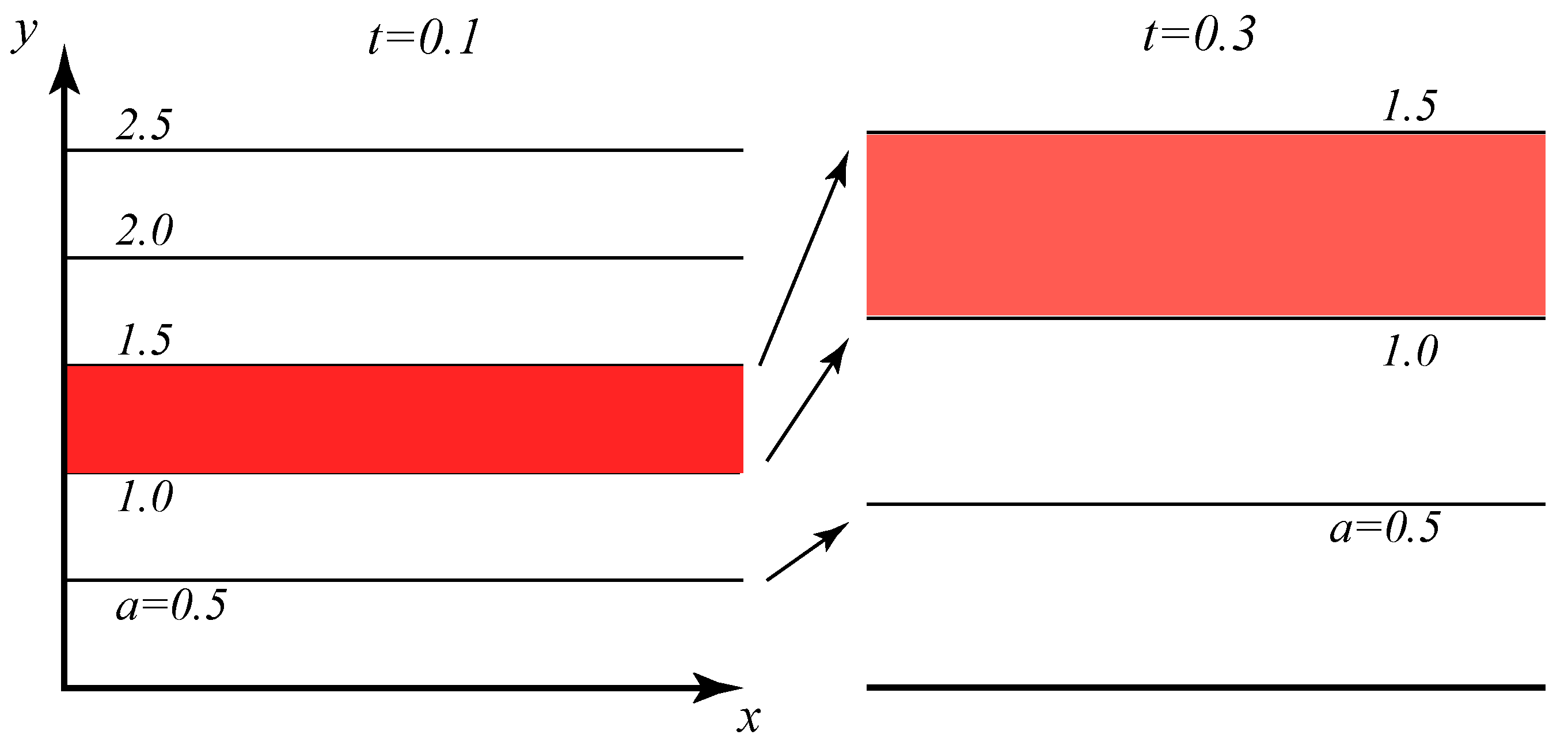
or x* = const. and y* = at1/2. One may now trace any contour y* = y*(x*,t) that evolves under Equation (21), an obvious first choice being the parallel contours y* = at1/2 parameterized by a, with . Note that the movement of the contours is independent of viscosity. All such contours initially lie at boundary (y = 0), but they explode into the fluid at t = 0+ and migrate towards positive y thereafter (Figure 10). The infinite speed of the leading contour is simply a reflection of the property of solutions to the parabolic equation, in which a sudden change at a boundary has an immediate impact at all finite distances from the boundary. The distance between any two contours a1 and a2 grows in proportion to t1/2 while the total amount of vorticity between the two remains constant. Thus, the vorticity moves away from the boundary and is diluted as it does so. Alternatively, one could have chosen a more complex contour, perhaps a circle, and seen that it becomes elongated in the y-direction as t increases.
It is also instructive to compute the rate at which enstrophy V = ζ2/2 moves into the fluid. Multiplication of Equation (20) by ζ results, after some rearrangement, in
so that now C = V, , and
Therefore, enstrophy moves into the domain at twice the speed of vorticity, but is dissipated as it does so.
Similar calculations can be done with momentum u and kinetic energy u2/2, resulting in the observation that energy moves twice as fast as momentum but is subject to a dissipation that momentum does not feel. In addition, v* < 0 for both scalars, so that the contours of zero flux move towards the boundary (which acts both as a sink of momentum and energy, but a source of vorticity and enstrophy).
2.3. A Turbulent Model of the Antarctic Circumpolar Current
We now consider the turbulent flow captured in an f-plane, continuously stratified model of wind driven flow in a channel ([46] and Figure 11). The model is motivated by the Antarctic Circumpolar Current but is implemented for Northern Hemisphere rotation, so that f > 0 and the surface Ekman transport is to the right of the wind stress. The channel is periodic in x and has rigid walls at y = 0, Ly. The flow is spun up from rest through the application of a wind stress in the positive x-direction proportional to sin2(πy/Ly). There is no buoyancy forcing and a linear drag is imposed at the bottom. The westerly surface winds create southward Ekman transport, leading to downwelling near the south wall (and upwelling at the north wall). The resulting isothermal tilt gives rise to a geostrophically balanced jet that becomes baroclinically unstable. In the simulation shown in Figure 11, the instability has equilibrated, and a statistically steady state is reached in which the dominant features are an eastward propagating meander and an accompanying anticyclonic eddy (lower left). Smaller coherent eddies can also be seen in both the southern and northern parts of the channel.
There are a number of dynamically relevant and interesting fluxes that one would like to measure in this strongly 3D flow. The authors in [46] draw particular attention to the generation of internal waves by larger scale motions. Here the flow field will be used to produce a simple example of methodology, in particular the time filtering and the properties of the residual velocity field. In order to maintain simplicity we will continue to work in 2D by considering only depth-averaged fields, leaving the more complex 3D fluxes for consideration in later work. Since there is no thermodynamic forcing in the simulation, a natural scalar quantity to examine is buoyancy: b = −g(ρ − ρo)/ρ. Note that buoyancy flux is essentially mass flux, so we are close in some sense to the volume flux calculations that are traditionally considered in lobe analysis.
In the model, the thermodynamic equation takes the form
where κ(8) and κ(4) are the horizontal and vertical hyper-diffusivities, respectively.
With the condition of incompressibility we obtain the flux form
The normal component of the buoyancy flux vector is set to zero on the sidewalls, and total volume integral of b is conserved to a high degree of accuracy. The low pass filtered version is
and its vertical average, denoted by 〈 〉 is
with
We first consider a comparison between the unfiltered, depth-average horizontal velocity field 〈u〉 = 〈u〉i + 〈v〉j and the residual velocity field computed using a Gaussian, low pass filter with a window T = 3.7 days. Snapshots of the forward FTLE fields for and for 〈u〉 are shown in Figure 12a,b. The maximizing FTLE ridges are suggestive of barriers associated with the hyperbolic-type LCSs or finite-time manifolds, whereas troughs in the FTLE fields at mid-jet (Figure 12a,c) are suggestive of barriers associated with the parabolic-type LCSs or shearless trajectories. These properties are backed up by independent calculations discussed below. Figure 12a contains information about the depth-averaged transport of mean (time-average) buoyancy whereas Figure 12b contains information about the depth-averaged transport of material. Note that although the anticyclonic eddy is apparent in the lower left corner of each panel (and more prominently in the 〈u〉 fields) the meandering jet is clear only in the panels showing . Cross jet material transport is therefore clearly indicated in the 〈u〉 fields, but the fields suggest that the jet is a barrier to mean buoyancy transport. Thus, if Lagrangian drifters were released on one side of the jet, some would cross to the other side. However, the FTLE troughs of the depth–integrated time-averaged residual velocity suggest that this parcel dispersion does not result in any residual transport of mean depth-averaged buoyancy: the associated “eddy” flux is balanced by the other terms in the residual flux vector, including the contribution from the mean cross-channel circulation and the explicit diffusion and hyper-diffusion terms. This cancellation is an expected consequence of the channel walls. It is also believed to take place in the Antarctic Circumpolar Current, where the wind and buoyancy forcing give rise to a mean meridional circulation that tends to steepen isopycnals, whereas baroclinic instability generates an eddy flux that tends to flatten isopycnals.
Further insight into the transport of mean buoyancy and the role of lobes can be found in Figure 12c in which the forward and backward FTLE fields for the residual velocity are overlain, giving the viewer an indication of regions of hyperbolicity and the expected geometry of intersecting finite-time stable and unstable manifolds of the hyperbolic trajectories within those regions. Note the region of strong hyperbolicity near x = 1.5 × 10⁵ and y = 0.5 × 10⁵ and the suggestion of a heteroclinic structure surrounding the anticyclonic gyre. In addition to looking at FTLE ridges, the finite-time manifolds emanating from the hyperbolic region have also been computed using a direct method, where they were “grown” from sets of initial conditions surrounding the hyperbolic core region. These are shown as color curves in Figure 12d, with blue/red representing stable/unstable directions. The red and blue curves fall right on top of FTLE ridges if the two images are superimposed. This calculation insures the attractive property of the FTLE ridges and confirms that ridges are hyperbolic in nature rather than associated with shear. The lobes formed by the intersections of the curves carry mean buoyancy into and out of the anticyclonic eddy. The exchange appears to be confined to the outer edges, and there is no evidence of penetration into the eddy center.
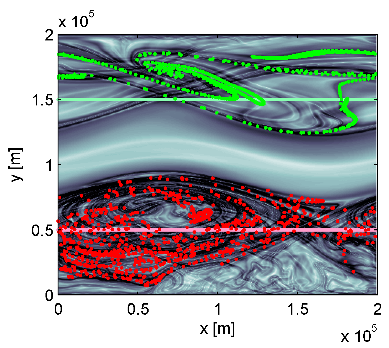
As a further confirmation that the meandering jet core acts as a barrier to mean buoyancy flux, we consider the advection by of the green and pink contours (Figure 13), initially aligned along the channel and lying to the north and south of the jet core. By definition of , the contours are barriers to average buoyancy flux, as are the channel side walls, so that the total buoyancy in any region bounded by a contour and a wall, or between the two contours, remains fixed as the contours evolve. The movement of a contour across the jet core would indicate a cross-jet buoyancy flux, but the contour positions after 71 days (dotted sets in Figure 13) indicates that this does not happen. This result is consistent with the behavior suggested by the troughs in the FTLE fields at mid-jet and by failure of the direct manifolds (Figure 12) to penetrate into the jet region, namely that the jet acts as a barrier to mean buoyancy flux.
Naturally, it would be of great interest to extend this analysis to 3D in order to pin down the depths at which exchange is taking place and to examine fluxes of other dynamically relevant quantities. This is well beyond the present scope.
3. Materials and Methods
Readers may consult [46] for a description of the numerical model used to produce the results in Section 3.3.
4. Discussion and Conclusions
The above examples are just an introduction to what may be a fruitful diagnostic that could help one understand scalar fluxes in complex flows through extension of the concept of a Lagrangian barrier to non-Lagrangian trajectories, and through the use of filtering in time. Though promising, the approach raises significant technical and interpretative challenges. For one thing, the residual velocity field is generally divergent/convergent (or “non-divergence free”, as one colleague likes to say) and, for simulations that resolve the ocean submesoscale, substantially 3D. The zoology of fixed points is thus considerably richer than in two-dimensional, incompressible flows and the assumptions that underpin the concepts of manifolds and Lagrangian coherent structures may have to be rethought. There is hope that this aspect might attract the attention of talented mathematicians.
A question that always arises in connection with the methodology is how to resolve the nonuniqueness of the flux vector. In some cases, boundary or initial conditions may be informative. For example, we could have added a nondivergent buoyancy flux in the cross-channel direction to the flux vector in Equation (27), but this would have violated the condition of zero buoyancy flux through the channel sidewalls. In cases where uncertainty remains, one may find it helpful to carefully consider the scientific question that led to consideration of the property flux in the first place. In our example with buoyancy flux, our primary interest is in cross-channel (y) transport. Alternatively, we could have added to our a y-dependent flux in the x-direction without altering Equation (27) and without violating any boundary conditions. This would have augmented the along-channel component of , which would have changed the way that contours are advected but it wouldn’t alter the conclusions about cross-channel transport. In fact, there may be instances in which such augmentation may be used to computational advantage. If the x-component of the original is highly sheared, for example, advected contours will rapidly stretch and filament. It may be desirable to remove this feature by subtracting a non-divergent flux vector that removes much of the shear.
In some applications the source/sink term (S in Equation (2)) may be sufficiently large that it dominates the evolution of the tracer. This situation could occur, for example, for nutrient limited biological scalars. In this case, the tracking of the transport barriers for the scalar flux may not be particularly helpful. Fortunately, there are cases in which S may be written as the divergence of a flux and absorbed in to the scalar flux vector F.
Our approach also attempts to achieve simplification through time filtering. (One could further smooth by filtering in space, but we have not gone this route.) The result is a relation (Equation (12)) guaranteeing that in the absence of sources and sinks, the total amount of time filtered scalar concentration will be conserved within moving barriers computed from the residual velocity field. (A similar assumption holds for any system that involves Reynolds time averaging over turbulent scales.) The interpretation of the results of time filtering may depend on the width T of the filter window: in our study T was chosen to be large enough to smooth the finest scales but not so large that the gyre and jet meanders were smoothed.
Acknowledgments
The authors are grateful for support through DOD (MURI) Grant N000141110087, administered by the Office of Naval Research. We also thank two reviewers for thoughtful suggestions and George Haller for pointing out the result listed at the end of Section 2.1.
Author Contributions
Larry Pratt wrote the manuscript and is responsible for the theory (Section 2.1) and the example of Section 2.2. Roy Barkan set up the numerical code and did the simulations leading to the example of Section 2.3. Irina Rypina calculated the FTLE fields and manifolds and produced Figure 12 and Figure 13. Both Barkan and Rypina edited paper and made helpful observations.
Conflicts of Interest
The authors declare no conflict of interest.
References
- Haller, G.; Beron-Vera, F.J. Geodesic theory of transport barriers in two-dimensional flows. Phys. D 2012. [Google Scholar] [CrossRef]
- Haller, G.; Beron-Vera, F.J. Coherent Lagrangian vortices: The black holes of turbulence. J. Fluid Mech. 2013, 731, R4. [Google Scholar] [CrossRef]
- Beron-Vera, F.J.; Wang, Y.; Olascoaga, M.J.; Goni, G.J.; Haller, G. Objective identification of oceanic eddies and the Agulhas leakage. J. Phys. Oceanogr. 2013, 43, 1426–1438. [Google Scholar]
- Wang, Y.; Olascoaga, M.J.; Beron-Vera, F.J. Coherent water transport across the South Atlantic. Geophys. Res. Lett. 2015, 42, 4072–4079. [Google Scholar]
- Rom-Kedar, V.; Leonard, A.; Wiggins, S. An analytical study of transport, mixing, and chaos in an unsteady vertical flow. J. Fluid Mech. 1990, 214, 347–394. [Google Scholar]
- Rom-Kedar, V.; Wiggins, S. Transport in two-dimensional maps. Arch. Ration. Mech. Anal. 1990, 109, 239–298. [Google Scholar]
- Samelson, R.M.; Wiggins, S. Lagrangian Transport in Geophysical Jets and Waves: The Dynamical Systems Approach; Springer: Berlin, Germany, 2006; p. 147. [Google Scholar]
- Haller, G. Lagrangian Coherent Structures. Annu. Rev. Fluid Mech. 2015, 47, 137–162. [Google Scholar]
- Rypina, I.I.; Pratt, L.J.; Pullen, J.; Levin, J.; Gordon, A. Chaotic advection in an archipelago. J. Phys. Oceanogr. 2012, 40, 1988–2006. [Google Scholar] [CrossRef]
- Rogerson, A.M.; Miller, P.; Pratt, L.J.; Jones, C.K.R.T. Lagrangian motion and fluid exchange in a barotropic meandering jet. J. Phys. Oceanogr. 1999, 29, 2635–2655. [Google Scholar] [CrossRef]
- Poje, A.C.; Haller, G. Geometry of cross-stream mixing in a double-gyre ocean model. J. Phys. Oceanogr. 1999, 29, 1649–1665. [Google Scholar] [CrossRef]
- Coulliette, C.; Wiggins, S. Intergyre transport in a wind-driven, quasigeostrophic double gyre: An application of lobe dynamics. Nonlinear Process. Geophys. 2001, 8, 69–94. [Google Scholar] [CrossRef]
- Deese, H.E.; Pratt, L.J.; Helfrich, K.R. A laboratory model of exchange and mixing between western boundary layers and subbasin recirculation gyres. J. Phys. Oceanogr. 2002, 32, 1870–1889. [Google Scholar] [CrossRef]
- Rypina, I.I.; Brown, M.J.; Kocak, H. Transport in an idealized three-gyre system with an application to the Adriatic Sea. J. Phys. Oceanogr. 2009, 39, 675–690. [Google Scholar] [CrossRef]
- Haller, G.; Hadjughasem, A.; Farazmand, M.; Huhn, F. Defining coherent vortices objectively from the vorticity. J. Fluid Mech. 2016, 795, 136–173. [Google Scholar] [CrossRef]
- Miller, P.D.; Pratt, L.J.; Helflrich, K.R.; Jones, C.K.R.T. Chaotic transport of mass and potential vorticity for an island circulation. J. Phys. Oceanogr. 2002, 32, 80–102. [Google Scholar] [CrossRef]
- Koh, T.Y.; Plumb, P.A. Lobe dynamics applied to barotropic Rossby wave breaking. Phys. Fluids 2000, 12, 1518–1528. [Google Scholar] [CrossRef]
- Branicki, M.; Kirwan, A.D. Stirring: The Eckart paradigm revisited. Int. J. Eng. Sci. 2010, 48, 1027–1042. [Google Scholar] [CrossRef]
- Haller, G.; Poje, A.C. Finite time transport in aperiodic flows. Phys. D 1998, 119, 352–380. [Google Scholar] [CrossRef]
- Haller, G. Lagrangian coherent structures from approximate velocity data. Phys. Fluids 2002, 14, 1851–1861. [Google Scholar] [CrossRef]
- Rypina, I.I.; Brown, M.G.; Beron-Vera, F.J.; Kocak, H.; Olascoaga, M.J.; Udovydchenkov, I.A. Robust transport barriers resulting from strong Kolmogorov-Arnold-Moser stability. Phys. Rev. Lett. 2007, 98, 104102. [Google Scholar] [CrossRef] [PubMed]
- Coulliette, C.; Lekien, F.; Paduan, J.D.; Haller, G.; Marsden, J.E. Optimal Pollution Mitigation in Monterey Bay Based on Coastal Radar Data and Nonlinear Dynamics. Environ. Sci. Technol. 2007, 41, 6562–6572. [Google Scholar] [CrossRef] [PubMed] [Green Version]
- Shadden, S.C.; Lekien, F.; Marsden, J.E. Definition and properties of Lagrangian coherent structures from finite-time Lyapunov exponents in two-dimensional aperiodic flows. Phys. D 2005, 212, 271–304. [Google Scholar] [CrossRef]
- Mezic, I.; Loire, S.; Fonoberov, V.A.; Hogan, P. A New Mixing Diagnostic and Gulf Oil Spill Movement. Science 2010, 330, 486–489. [Google Scholar] [CrossRef]
- Froyland, G.; Padberg, K.; England, M.H.; Treguier, A.M. Detection of coherent oceanic structures via transfer operators. Phys. Rev. Lett. 2007, 98, 224503. [Google Scholar] [CrossRef] [PubMed]
- Froyland, G.; Horenkamp, C.; Rossi, V.; Santitissadeekorn, N.; Gupa, A.S. Three-dimensional characterization and tracking of an Agulhas Ring. Ocean Model. 2012, 52–53, 69–75. [Google Scholar] [CrossRef]
- Budisic, M.; Mezic, I. Geometry of the ergodic quotient reveals coherent structures in flows. Phys. D 2012, 241, 1255–1269. [Google Scholar] [CrossRef]
- Fabregat, A.; Mezic, I.; Poje, A.C. Finite-time Partitions for Lagrangian Structure Identification in Gulf Stream Eddy Transport. Phys. Rev. F Fluids 2016, in press. [Google Scholar]
- Mancho, A.M.; Small, D.; Wiggins, S.; Ide, K. Computation of stable and unstable manifolds of hyperbolic trajectories in two-dimensional, aperiodically time-dependent vector fields. Nonlinear Process. Geophys. 2003, 11, 17–33. [Google Scholar] [CrossRef]
- Rypina, I.; Scott, A.; Pratt, L.J.; Brown, M.F. Investigating the connection between complexity of isolated trajectories and Lagrangian coherent structures. Nonlinear Process. Geophys. 2011, 18, 977–987. [Google Scholar] [CrossRef]
- Farazmand, M.; Haller, G. Polar rotation angle identifies elliptic islands in unsteady dynamical systems. Phys. D 2016, 315, 1–12. [Google Scholar] [CrossRef]
- Mazloff, M.R.; Heimbach, P.; Wunsch, C. An eddy-permitting Southern Ocean state estimate. J. Phys. Oceanogr. 2010, 40, 880–899. [Google Scholar] [CrossRef]
- Mezic, I. Break-up of invariant surfaces in action-angle-angle maps and flows. Phys. D 2001, 154, 51–67. [Google Scholar] [CrossRef]
- Pratt, L.J.; Rypina, I.I.; Özgökmen, T.; Childs, H.; Bebieva, T. Chaotic Advection in a Steady, 3D, Ekman-Driven Circulation. J. Fluid Mech. 2014, 738, 143–183. [Google Scholar] [CrossRef]
- Rypina, I.I.; Pratt, L.J.; Wang, P.; Ozgokmen, T.M.; Mezic, I. Resonance phynomena in a time-dependent, three-dimensional model of an idealized eddy. Chaos 2015, 25. [Google Scholar] [CrossRef] [PubMed]
- Solomon, T.H.; Mezic, I. Uniform resonant chaotic mixing in fluid flows. Nature 2003, 425, 376–380. [Google Scholar] [CrossRef] [PubMed]
- Ide, K.; Wiggins, S. Transport induced by mean-eddy interaction: I. Theory and relation to Lagrangian lobe dynamics. Commun. Nonlinear Sci. Simul. 2015, 20, 516–535. [Google Scholar] [CrossRef]
- Ide, K.; Wiggins, S. Transport induced by mean-eddy interaction: II. Anallysis of transport processes. Commun. Nonlinear Sci. Simul. 2015, 20, 794–806. [Google Scholar] [CrossRef]
- Rypina, I.I.; Pratt, L.J.; Lozier, S.M. Near-surface transport pathways in the North Atlantic Ocean. J. Phys. Oceanogr. 2011, 41, 911–925. [Google Scholar] [CrossRef]
- Poje, A.C.; Haza, A.C.; Ozgokmen, T.M. Resolution dependent relative dispersion statistics in a hierarchy of ocean models. Ocean Model. 2010, 31, 36–50. [Google Scholar] [CrossRef]
- Beron-Vera, F.J.; Olascoaga, M.J.; Haller, G.; Farazmand, M.; Trinanes, J.; Wan, Y. Dissipative inertial transport patterns near coherent Lagrangian eddies in the ocean. Chaos 2015, 25, 087412. [Google Scholar] [CrossRef] [PubMed]
- Beron-Vera, F.B.; Olascoaga, M.J.; Haller, G.; Trinanes, J.; Iskandarani, M.; Coelho, E.F.; Haus, B.K.; Huntley, H.S.; Jacobs, G.; Kirwan, A.D.; et al. Drifter motion in the Gulf of Mexico constrained by altimetric Lagrangian coherent structures. Geophys. Res. Lett. 2013, 40, 6171–6175. [Google Scholar]
- Pedlosky, J. Geophysical Fluid Dynamics, 2nd ed.; Springer-Verlag: Dordrecht, The Netherlands, 1987; p. 710. [Google Scholar]
- Leonard, A. Energy cascade in large-eddy simulations of turbulent fluid flows. Adv. Geophys. A 1974, 18, 237–248. [Google Scholar]
- Vallis, G.K. Atmospheric and Oceanic Fluid Dynamics; Cambridge University Press: Cambridge, UK, 2006; p. 745. [Google Scholar]
- Barkan, R.; Winters, K.B.; McWilliams, J.C. Stimulated Imbalance and the Enhancement of Eddy Kinetic Energy Dissipation by Internal waves. J. Phys. Oceanogr. 2016. submitted. [Google Scholar]
Figure 1.
Schematic of exchange in a dipole circulation. (a) Here the flow is steady and there is no material exchange between the two cells; (b) The flow is time-dependent and the gyres are no longer separated by a material boundary. Instead blue lobes (L1, L2, etc.) of material move left to right and are transported from the anticyclone to the cyclone. The uncolored lobes L−1, L−2, etc. are transported to the anticyclone from the cyclone. The solid arrows show the general direction of circulation. Dashed contours schematically indicate the outermost material contour marking the extent of the regular region within each gyre. (From [9] © American Meteorlogical Society. Used with permission.).
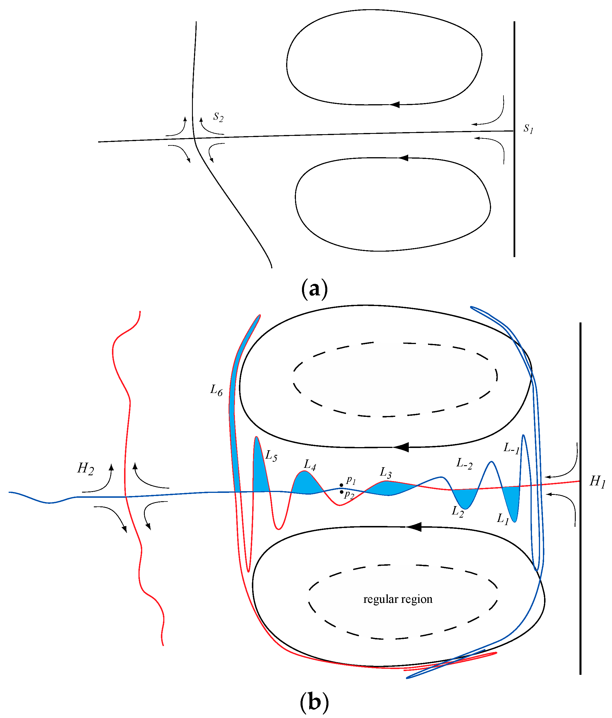
Figure 2.
Philippine Seas dipole with the geometry resembling the idealized example shown in Figure 1. Red and blue curves are finite-time analogs of the stable and unstable manifolds computed for a realistic numerical simulation of the Philippine Seas. The red curves emanate from hyperbolic regions close to the coastlines of a peninsula and 2 islands near x = 620. The blue curves emanate from an offshore hyperbolic region not shown, and from hyperbolic regions near the coasts. (From [9] © American Meteorlogical Society. Used with permission.).

Figure 3.
The finite volume lobes formed by intersecting manifolds in a 3D simulation of a Gulf of Mexico eddy. (Reprinted from [18], Copyright 2010, with permission from Elsevier.).
Figure 3.
The finite volume lobes formed by intersecting manifolds in a 3D simulation of a Gulf of Mexico eddy. (Reprinted from [18], Copyright 2010, with permission from Elsevier.).

Figure 4.
Forward and backward finite-time Lyapunov exponents (FTLEs) for the surface circulation according to a numerical simulation of the Philippine Seas. (From [9] © American Meteorlogical Society. Used with permission.).
Figure 4.
Forward and backward finite-time Lyapunov exponents (FTLEs) for the surface circulation according to a numerical simulation of the Philippine Seas. (From [9] © American Meteorlogical Society. Used with permission.).

Figure 5.
The red filamented surface material in (a) coalesces to form an eddy in (b) that remains coherent as it travels westward across the middle portion of the S. Atlantic (c); The distance covered between frames (b) and (c) is approximately 4000 km. (Courtesy of F. J. Beron-Vera, also see [4]).
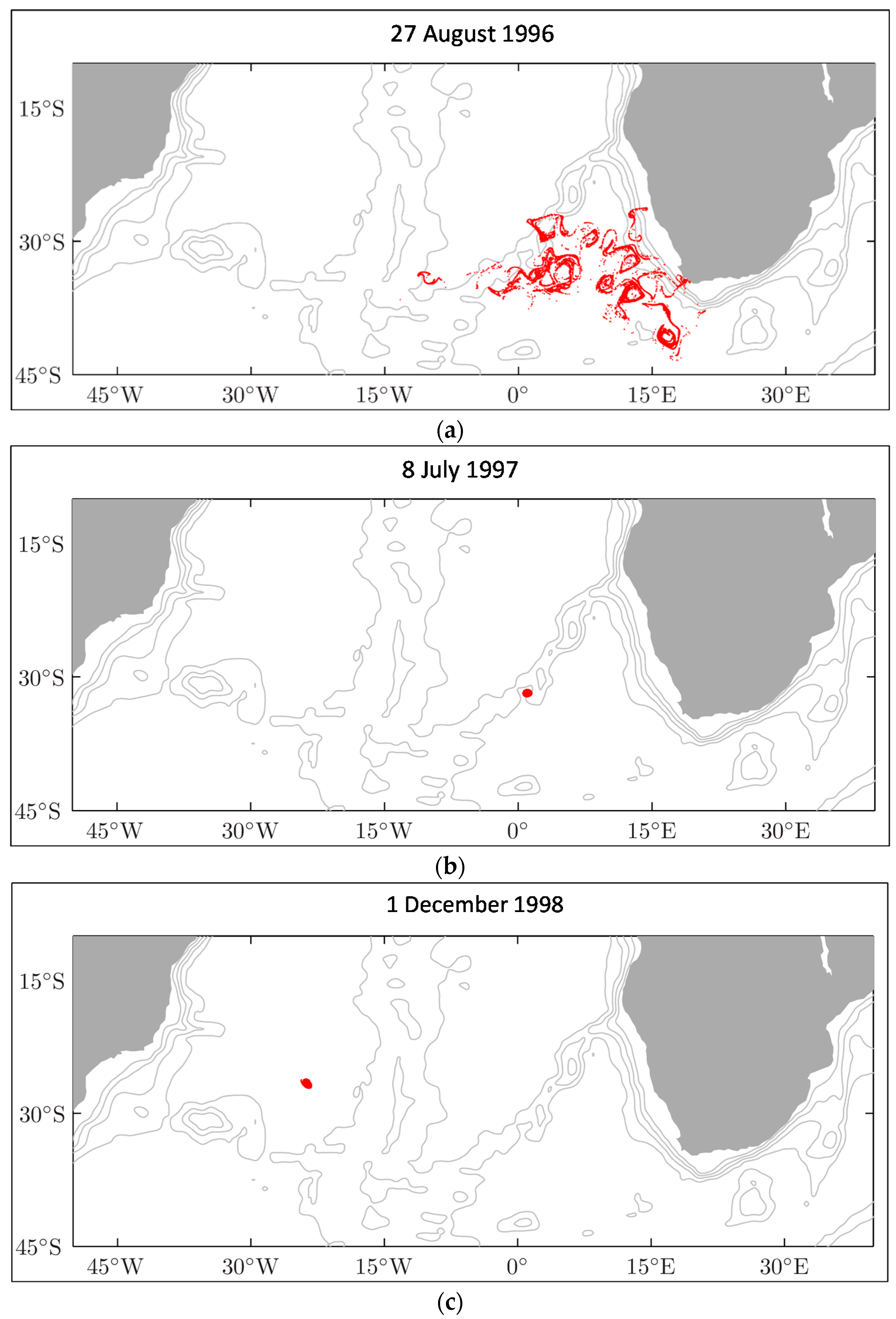
Figure 6.
The yellow surface is the boundary of a mesoscale eddy computed using the technique of [15] and based on the Southern Ocean state estimation model [32]. The boundary was found to remain coherent over at least 120 days. (From [15], reproduced with permission from Cambridge University Press.).

Figure 7.
(a) Schematic of the rotating cylinder flow, with the homogeneous fluid in the cylinder driven by a positive differential rotation of the lid. This forcing results in upwelling into a surface Ekman Layer, downwelling in sidewall layers, and collection and expulsion of trajectories in a bottom Ekman layer. Hypebolic stagnation points exist at the center of the bottom and top lids; (b) A chaotic trajectory (red) and two material barriers (green and blue, both tori) that arise when the lid stress is moved slightly off center. (All from [34], reproduced with permission from Cambridge University Press.).
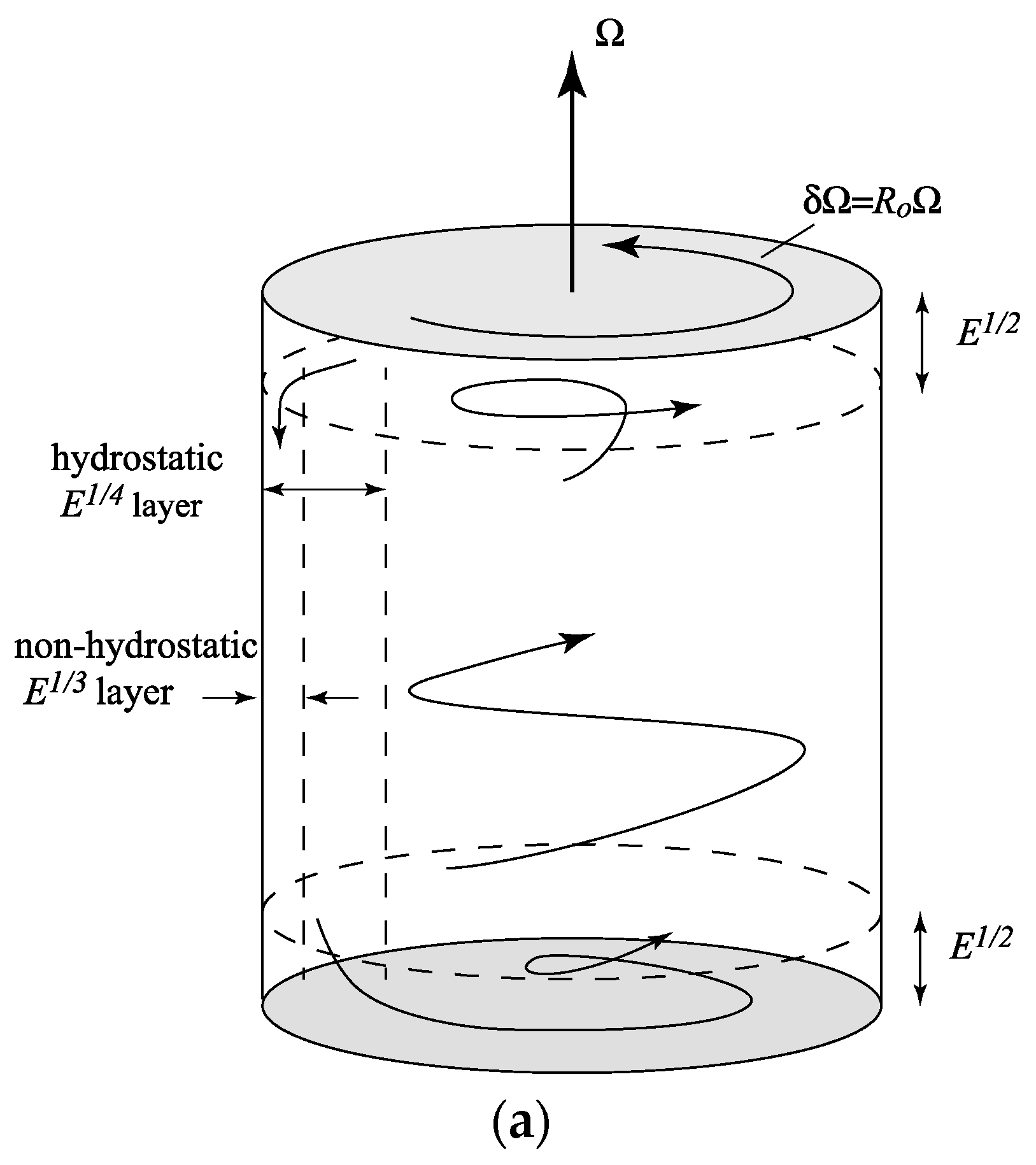
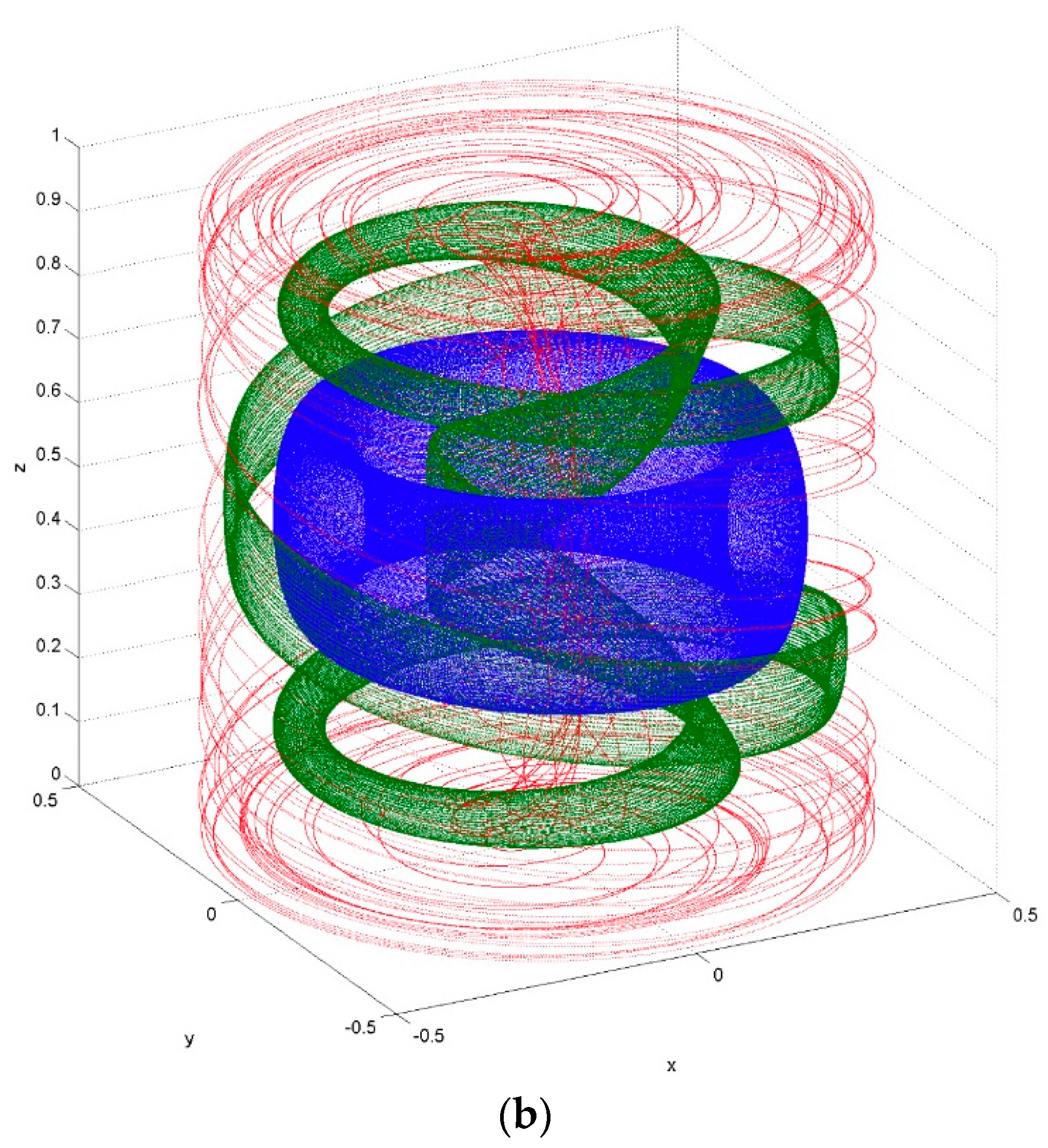
Figure 8.
Turnstile lobe exchange of fluid in and out of a boundary trapped gyre in a single-layer, wind-driven gyre on a β-plane. The blue lobe contains fluid transported from the interior to the exterior of the gyre, while the red lobe contains fluid that is being transported into the gyre. Both are responsible for carrying potential vorticity into and out of the gyre, which can cause the gyre to spin up or spin down. (From [16] © American Meteorlogical Society. Used with permission.).
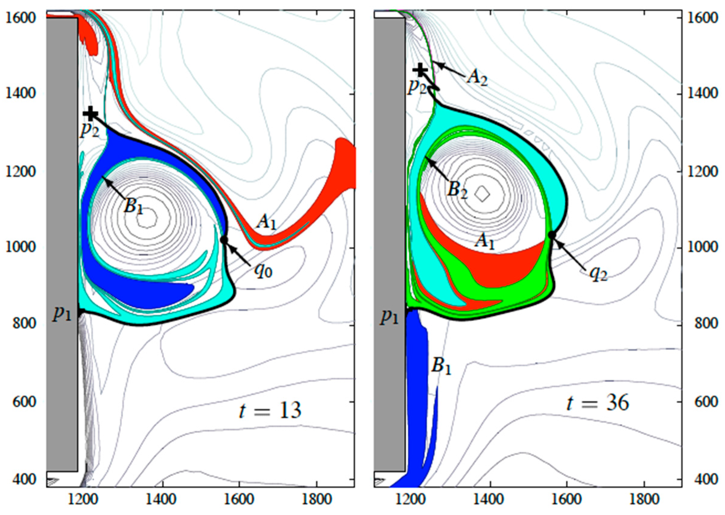
Figure 9.
Snapshot of forward-time FTLEs on 6 January 1993 based on surface velocities from the time-dependent AVISO satellite altimetry superposed on the drifter-based mean flow. The ridges ostensibly approximate finite-time unstable manifolds or hyperbolic-type LCS. Backward-time FTLEs (not shown) exhibit the same level of complexity. (From [39] © American Meteorlogical Society. Used with permission.).
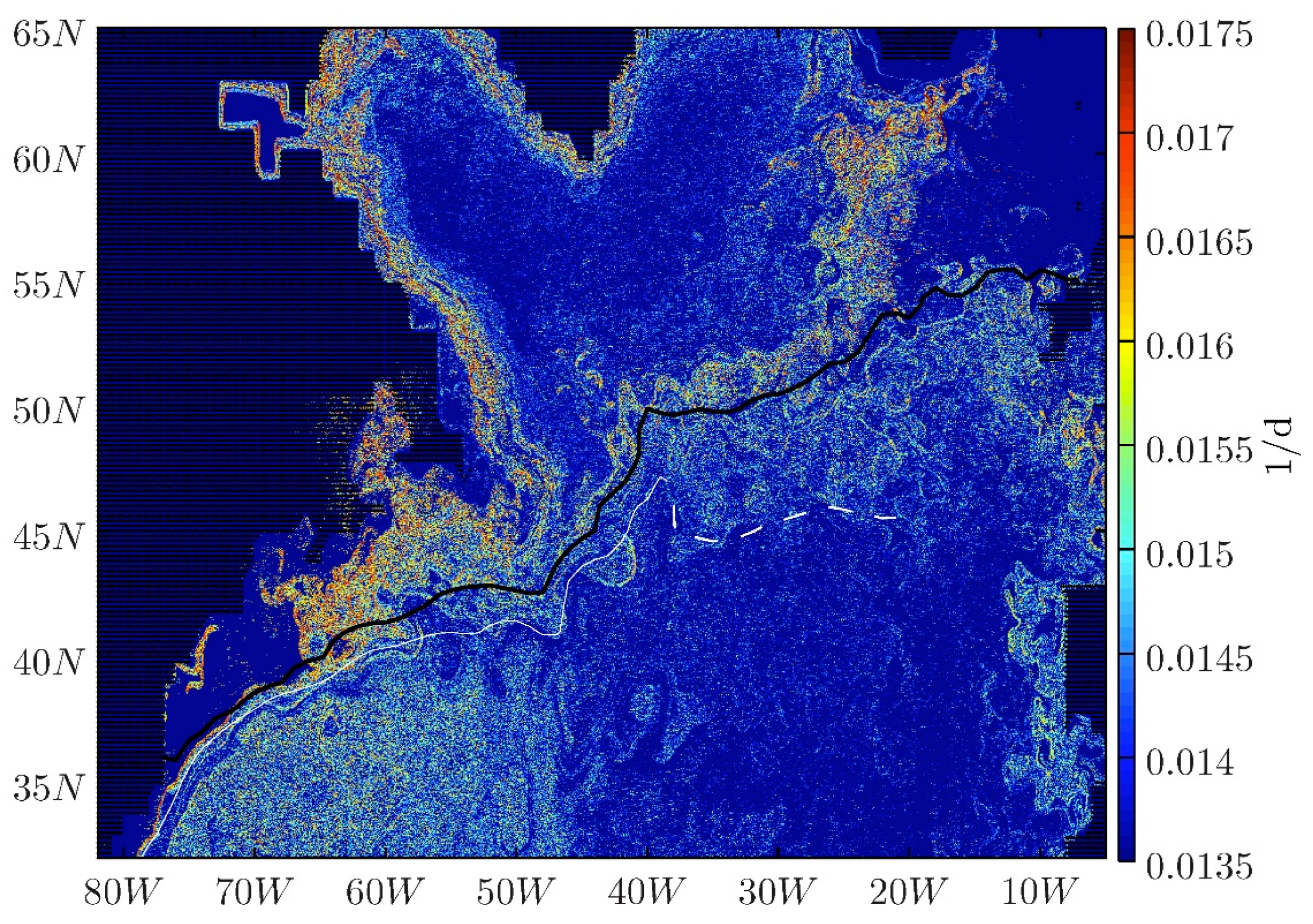
Figure 10.
Contours corresponding to different values of a, and at two different times. The total vorticity between two contours of different a remains fixed. As time progresses, the contours move away from the lower boundary, the distance between contours increases, and the vorticity is diluted.
Figure 10.
Contours corresponding to different values of a, and at two different times. The total vorticity between two contours of different a remains fixed. As time progresses, the contours move away from the lower boundary, the distance between contours increases, and the vorticity is diluted.

Figure 11.
The geometry, forcing and main circulation features from the zonal channel model. The color shows the vertical component of fluid vorticity, normalized by f. (Based on the model runs presented in [46]).
Figure 11.
The geometry, forcing and main circulation features from the zonal channel model. The color shows the vertical component of fluid vorticity, normalized by f. (Based on the model runs presented in [46]).
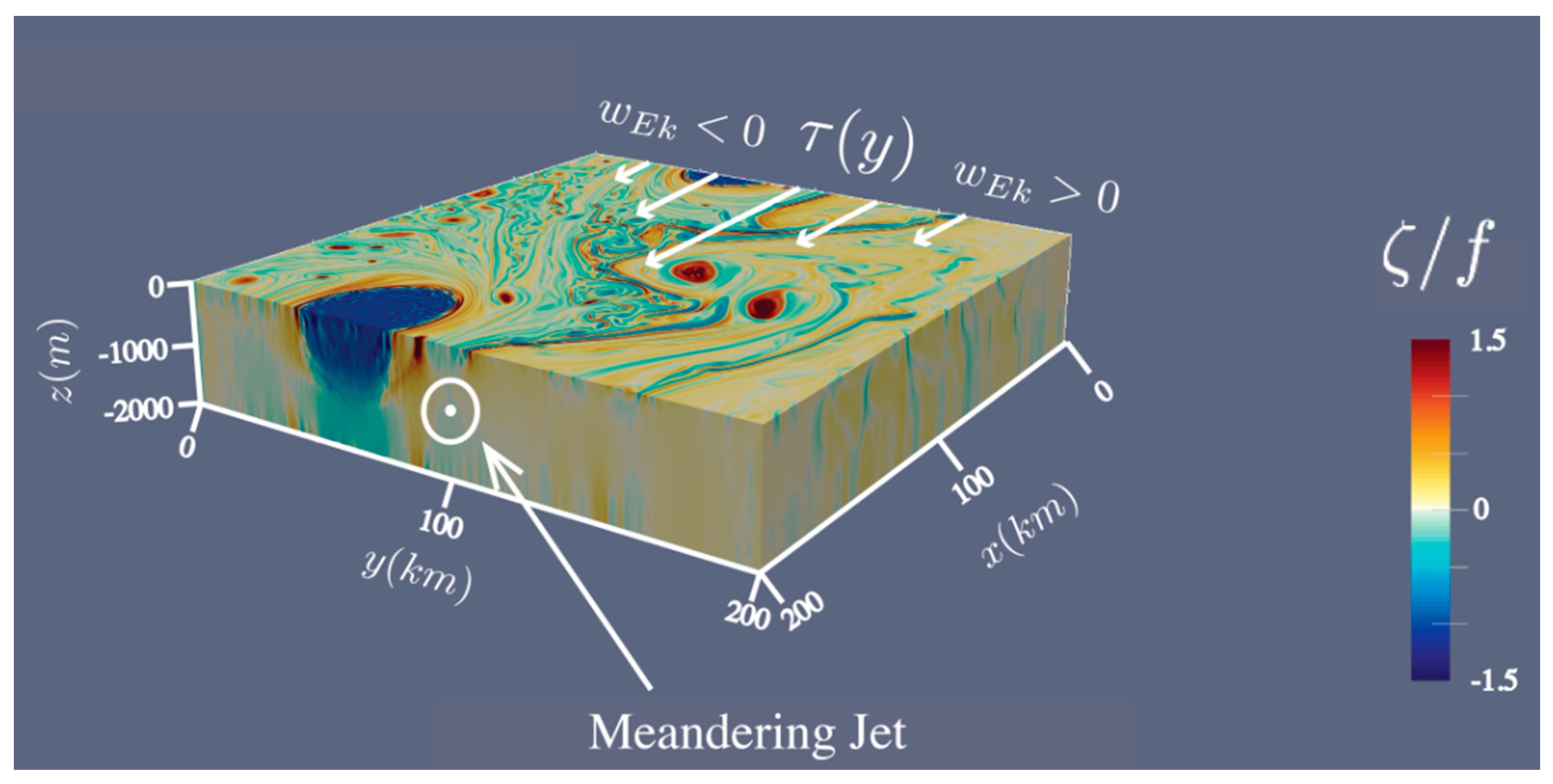
Figure 12.
(a) Forward FTLE fields for ; (b) Forward FTLE fields for 〈u〉; (c) Forward and backward FTLE fields for ; (d) Stable (blue) and unstable (red) manifolds grown from the hyperbolic region near x = 1.5 × 10⁵ for .
Figure 12.
(a) Forward FTLE fields for ; (b) Forward FTLE fields for 〈u〉; (c) Forward and backward FTLE fields for ; (d) Stable (blue) and unstable (red) manifolds grown from the hyperbolic region near x = 1.5 × 10⁵ for .
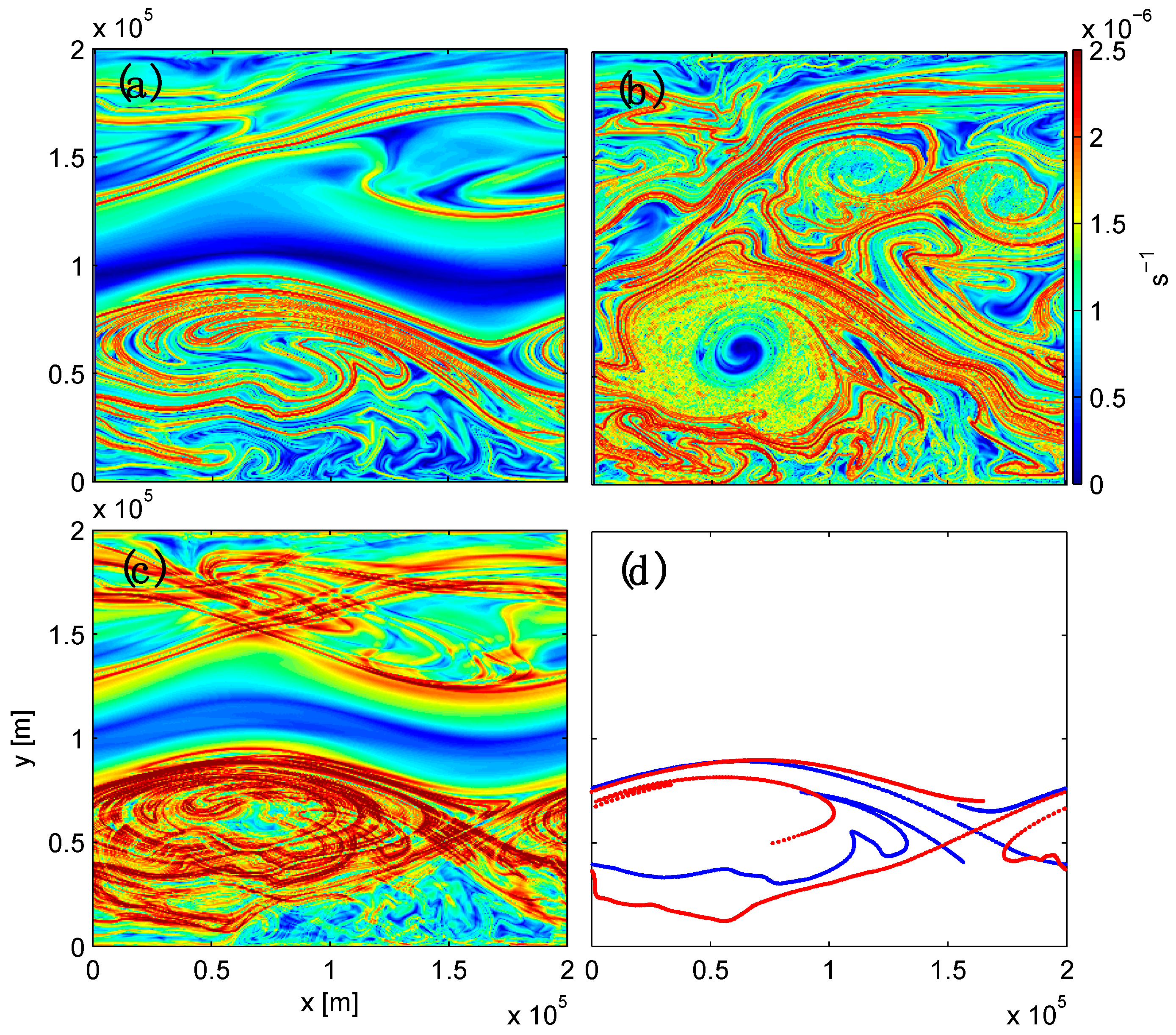
Figure 13.
The light green and pink contours, initially aligned along the channel, are advected by for 71 days, resulting in the bright green and red dotted sets. No cross-jet transport of mean buoyancy occurs.
Figure 13.
The light green and pink contours, initially aligned along the channel, are advected by for 71 days, resulting in the bright green and red dotted sets. No cross-jet transport of mean buoyancy occurs.
© 2016 by the authors; licensee MDPI, Basel, Switzerland. This article is an open access article distributed under the terms and conditions of the Creative Commons Attribution license ( http://creativecommons.org/licenses/by/4.0/).
Share and Cite
MDPI and ACS Style
Pratt, L.; Barkan, R.; Rypina, I. Scalar Flux Kinematics. Fluids 2016, 1, 27. https://doi.org/10.3390/fluids1030027
AMA Style
Pratt L, Barkan R, Rypina I. Scalar Flux Kinematics. Fluids. 2016; 1(3):27. https://doi.org/10.3390/fluids1030027
Chicago/Turabian StylePratt, Larry, Roy Barkan, and Irina Rypina. 2016. "Scalar Flux Kinematics" Fluids 1, no. 3: 27. https://doi.org/10.3390/fluids1030027