Article

Investigation of Slot-Burner Aerodynamics with Recessed-Type Nozzle Geometry

1
Faculty of Science, Engineering and Technology, Swinburne University of Technology, Victoria VIC 3122, Australia
2
Department of Mechanical Engineering, Islamic University of Technology, Gazipur-1704, Bangladesh
3
Mineral Resources, Commonwealth Scientific and Industrial Research Organisation (CSIRO), Victoria 3168, Australia
*
Author to whom correspondence should be addressed.
Fluids 2016, 1(2), 10; https://doi.org/10.3390/fluids1020010
Submission received: 19 February 2016 / Revised: 21 March 2016 / Accepted: 23 March 2016 / Published: 8 April 2016
(This article belongs to the Special Issue Computational Fluid Dynamics)

Abstract

:
The aerodynamics of fully turbulent jets supplied from rectangular slot-burners was modelled using the Reynolds Averaged Navier–Stokes (RANS) model. Three different turbulent models were considered, such as standard k-ε, RNG k-ε and Reynolds stress turbulence models. The recessed-type nozzle geometry was investigated to determine the effect of burner geometry on jet development. The slot-burner was based on physical models, which were designed to be representative of typical burner geometries found in tangentially-fired coal boilers. The study was validated against the physical models. The detailed flow field obtained from the simulations was used to explain the aerodynamic development of jets in such burners. It was found that the addition of a recess section to the nozzle geometry introduced significant changes to the flow due to complex pressure and mixing fields being set up inside the recess, which altered the jets once they exited into the open atmosphere.

1. Introduction

In general, combustion flames are found close to the nozzle area as combustion occurs in the main reaction zone in gas-fired and black coal-fired boilers [1,2,3,4,5]. It is found that some burning happens just after the brown-coal burner jets. This is due to the process of pyrolysis and devolatilization of the particles, though the behaviour of the turbulent characteristics is less important for combustion [6]. The aim of mixing is to heat the fuel and oxidizer elements by using the incoming heated flue gases and to supply the mixture to the reaction zone of the furnace. The near-field aerodynamics are still important in entrainment and in confirming the jets spread in the centre of the reactor at the appropriate position and with adequate momentum to create the swirl required to stabilize the flame in the centre. The level of burning in the burner area is lower, since the aerodynamics is necessarily decoupled from the possessions of strong chemical processes and radiative heat transfer, leading to flame temperatures that vary the physical conditions of the flow [3]. The dynamics of combustion is directly linked to flame characteristics in a moderately premixed burner, as demonstrated in [7,8]. Hence, constant temperature simulation can sensibly be predictable to provide a decent suggestion for how the jets from diverse burner geometries distribute the stream of fuel and oxidizer and blend it with the neighbouring hot flue gases within the reactor. Stabilization in combustion in a tangentially-fired brown coal boiler [9,10,11,12] is accomplished by positioning the burner jets in the furnace walls, so as to induce a vortex in the central region of the boiler (Figure 1) in which the majority of combustion occurs. A burner set may include several main burners located in a vertical plane, which commonly consists of a central or primary slot, injecting a fuel/air mixture, with secondary air slots located above and below. There is significant separation between the jets. Recently, the aerodynamics of a recessed rectangular slot-burner used in tangentially-fired furnaces by varying the jet velocity ratio in the presence of cross-flow was investigated [13,14]. A similar study was performed in a tangentially-fired furnace using slot burner in [15].
The object of this study is a recessed burner type, which is used in a large-scale power station located in Australia. The burners exhibited undesirable characteristics, operating in highly unsteady modes producing unstable and unpredictable flames, and under extreme circumstances, some of the burner-jets were found to impinge on the furnace walls, resulting in coal particles burning on the wall surface and leaving ash deposits, which slagged and reduced furnace efficiency. Previous non-recessed designs were operating well, with stable flames. Scaled-down physical models were investigated by the industries, in which structural models were prepared for relevant burner shapes. Constant temperature simulation was implemented on various types of isolated geometries. Modelling of 3D performances is significant in such types of complex flows, and if simulated accurately, the complete flow field estimation from a computational fluid dynamics model can deliver further understanding of the burner aerodynamics compared to real-life analysis. The objective of this investigation was to develop a precise and well-validated computational model of the constant temperature geometry and usage of the outcomes to improve the understanding of the field aerodynamics of the jets within the burner. This study was conducted using a commercial CFD package, ANSYS CFX. This understanding will be valuable for future burner designs.

2. Mathematical Modelling

CFD was used to model the fluid flow, which was subsonic, isothermal, single phase and fully turbulent. The resulting simplified Reynolds Averaged Navier–Stokes (RANS) system [16,17,18,19] of equations solved in this numerical model was for a constant density, constant temperature and unsteady flow. The closure of the RANS equation by the calculation of Reynolds stresses was achieved using the k-ε model of Jones and Launder [20], the Re-Normalisation Group (RNG) k-ε model of Yakhot and Orszag [21] and the Reynolds Stress Model (RSM) of Launder, Reece and Rodi [22]. Wall functions were applied based on the approach of Launder and Spalding [23].
In the present study, the wall-function method is employed to model the flow in the near-wall region. In the wall function approach, the viscosity affected sub-layer region is bridged by employing empirical formulas to provide near-wall boundary conditions for the mean flow and turbulence transport equations. These formulas connect the wall conditions (e.g., the wall shear stress) to the dependent variables at the near wall grid node, which is presumed to lie in the fully-turbulent region of the boundary layer. The major advantage of the wall-function approach is that it conserves valuable computer resources, and it avoids the need to account for viscous effects in the turbulence model.
The k-ε model: The k-ε model is the industry standard two-equation turbulence model. It is the most prominent turbulence model, which has been implemented in most general purpose CFD codes. It has been proven to be stable and numerically robust and has a well-established regime of predictive capability. This model provides good predictions for many flows of engineering interest. There are applications for which these models may not be suitable. Among these are: flows with boundary layer separation, flows with sudden changes in the mean strain rate, flows in rotating fluids and flows over curved surfaces.
k is the turbulence kinetic energy, defined as the variance of the fluctuations in velocity. It has dimensions of (L2·T−2), e.g., m2/s2. ε is the turbulence eddy dissipation and has dimensions of k per unit time (L2 T−3).
The k-ε model introduces two new variables into the system of equations. The governing equations based on the assumptions for the study are as follows:
The continuity equation:
u x + v y + w z = 0
The momentum equation:
x-component:
u t + ρ ( u u x + v u y + w u z ) = p x + μ e f f ( 2 u x 2 + 2 u y 2 + 2 u z 2 )
y-component:
v t + ρ ( u v x + v v y + w v z ) = p y + μ e f f ( 2 v x 2 + 2 v y 2 + 2 v z 2 )
z-component:
w t + ρ ( u w x + v w y + w w z ) = p z + μ e f f ( 2 w x 2 + 2 w y 2 + 2 w z 2 )
where p is the modified pressure given by:
p = p + 2 3 ρ × k
The k-ε model, like the zero equation model, is based on the eddy viscosity concept, so that,
μ eff = μ + μ t
where μ t is the turbulence viscosity. The k-ε model assumes that the turbulence viscosity is linked to the turbulence kinetic energy and dissipation via relation:
μ t = C μ   × ρ × k 2 ε
where Cμ = 0.09 is a k-ε turbulent model constant. The values of k and ε come directly from the differential transport equations for the turbulence kinetic energy and turbulence dissipation rate.
ρ [ k t + ( u k x + v k y + w k z ) ] μ eff σ k ( 2 k x 2 + 2 k y 2 + 2 k z 2 ) = P k ρ ε
ρ [ ε t + ( u ε x + v ε y + w ε z ) ] μ eff σ ε ( 2 ε x 2 + 2 ε y 2 + 2 ε z 2 ) = ε k ( C ε 1 P k C ε 2 ρ ε )
where Cε1 = 1.44, Cε2 = 1.92, σε = 1.3 are the k-ε turbulent model constants. Pk is the shear production due to turbulence, which for incompressible flow is given by the following equation. Here, UT is the transpose of the velocity vector matrix.
P k = μ t U · ( U + U T ) 2 3 · U ( 3 μ t · U + ρ k ) + P kb
The RNG k-ε model: The RNG k-ε model is an alternative to the standard k-ε model. It is based on the renormalizing group analysis of the Navier–Stokes equations. The transport equations for turbulence generation and dissipation are the same as those for the standard k-ε model, but the model constants differ, and the constant Cε1 is replaced by the function Cε1RNG. The transport equation for the turbulence dissipation becomes:
( ρ ε ) t + · ( ρ U ε ) = · [ ( μ + μ t σ ε RNG ) ε ] + ε k ( C ε 1 RNG P k C ε 2 RNG ρ ε )
where Cε1RNG = 1.42 − fn, where fn is the RNG k-ε model coefficient and is given by,
f n = η ( 1 η 4.38 ) ( 1 + β RNG ε )
η = P k ρ C μ RNG ε
The Reynolds Stress Models (RSM): Two-equation turbulence models (k-ε and k-ω based models) offer good predictions of the characteristics and physics of most flows of industrial relevance. In flows where the turbulent transport or non-equilibrium effects are important, the eddy viscosity assumptions are no longer valid, and the results of eddy viscosity models might be inaccurate. Reynolds stress or Second Moment Closure (SMC) models naturally include the effects of streamline curvature, sudden changes in the strain rate, secondary flows or buoyancy compared to turbulence models using the eddy viscosity approximation. The Reynolds stress model is used in the following types of flow: free shear flows with strong anisotropy, like those with a strong swirl component. This includes flows in rotating fluids, flows with sudden changes in the mean strain rate, flows where the strain fields are complex and reproduce the anisotropic nature of the turbulence itself, flows with strong streamline curvature, secondary flows and buoyant flows.
Reynolds stress models have shown superior predictive performance compared to eddy-viscosity models in these cases. This is the major justification for Reynolds stress models, which are based on transport equations for the individual components of the Reynolds stress tensor and the dissipation rate. These models are characterized by a high degree of universality. Theoretically, Reynolds stress models are more suited to complex flows; however, practice shows that they are often not superior to two-equation models.
These models are based on transport equations for all components of the Reynolds stress tensor and the dissipation rate. They are suitable for strongly anisotropic flows. These models do not use the eddy viscosity hypothesis, but solve an equation for the transport of Reynolds stresses in the fluid. Their general use has been limited because of the increased number of additional transport equations, which leads to a reduced numerical stability and requires increased computational effort. Algebraic Reynolds stress models solve algebraic equations for the Reynolds stresses, whereas differential Reynolds stress models solve differential transport equations individually for each Reynolds stress component. The exact production term and the inherent modelling of stress anisotropies theoretically make Reynolds stress models more suited for complex flows; however, practice shows that they are often not superior to two-equation models. Reynolds stress models can be suited to flows where the strain fields are complex and reproduce the anisotropic nature of the turbulence itself. They are particularly useful where there is strong streamline curvature or swirl. The Reynolds averaged momentum equations for the mean velocities are:
ρ U t + · ( ρ   U U ) · ( μ U ) = p · ( ρ u u ¯ ) + B
where p‘’ is a modified pressure, B is the sum of body forces and the fluctuating Reynolds stress contribution is ρ u u ¯ . Unlike the eddy viscosity model, the modified pressure has no turbulence contribution and is related to the static (thermodynamic) pressure by:
p = p + · U ( 2 3 μ ξ )
In the differential stress model, u u ¯ is made to satisfy a transport equation. A separate transport equation must be solved for each of the six Reynolds stress components of ρ u u ¯ . The differential equation Reynolds stress transport is:
ρ u u ¯ t + · ( ρ   u u ¯ U ) · ( ρ C k ε u u ( u u ) T ) = ( P + G + ϕ 2 3 δ ρ ε )
where P and G are shear and buoyancy turbulence production terms of the Reynolds stress, respectively, φ is the pressure-strain tensor and C is a constant.
The standard Reynolds stress model is based on the ε-equation and can be written as:
ρ u u ¯ t + · ( ρ   u u ¯ U ) = ( P + ϕ + · ( ( μ + 2 3 c s ρ k 2 ε ) u u ¯ ) 2 3 δ ρ ε )
which can be written in index notation as:
t ( ρ u i u j ¯ ) + x k ( U k ρ u i u j ¯ ) = P ij + ϕ ij + x k [ ( μ + 2 3 c s ρ k 2 ε ) u i u j ¯ x k ] 2 3 δ ij ρ ε
where φij is the pressure strain correlation, and P, the exact production term, is given by:
P = ρ ( u u ¯ ( U ) T + ( U ) u u )
As the turbulence dissipation appears in the individual stress equations, an equation for ε is required. This now has the form:
( ρ ε ) t + x k ( ρ U k ε ) = ε k ( C ε 1 P C ε 2 ρ ε ) + x k [ ( μ + μ t σ ε ) ε x k ]
In these equations, the anisotropic diffusion coefficients of the original models are replaced by an isotropic formulation, which increases the robustness of the Reynolds stress model.
One of the most important terms in Reynolds stress models is the pressure strain correlation, φij. The pressure strain correlations can be expressed in the general form:
ϕ ij = ϕ ij 1 + ϕ ij 2
where:
ϕ ij 1 = ρ ε ( C s 1 a + C s 2 ( aa 1 3 a · a δ ) )
ϕ ij 2 = C r 1 Pa + C r 2 ρ kS C r 3 ρ kS a · a 2 + C r 4 ρ k ( aS T + Sa T 2 3 a · S δ ) + C r 5 ρ k ( aW T + Wa T )
a = u u ¯ k 2 3 δ
S = 1 2 ( U + ( U ) T )
W = 1 2 ( U ( U ) T )
In this formulation, a is the anisotropy tensor, S is the strain rate and W is the vorticity. Two discretization schemes were employed, a hybrid linear upwind/central differencing and CCCT (Curvature Compensated Convective Transport), which is a modified QUICK (Quadratic Upwind Differencing) scheme, which is bounded to prevent non-physical overshoots in k and epsilon. The SIMPLER (SIMPLE-Revised) method was used as the solution algorithm [24], and the Rhie and Chow [25] method was employed to prevent chequerboard oscillations in the pressure.

3. Physical Structure and Burner Geometry

The burners modelled in this study were based on the physical models of Perry and Hausler given in [26], where four different models having different geometry were considered, called A, B, C and D. A brief description of all of the geometries is summarized in Table 1. Only Geometry D was modelled in the current study, and Figure 2 illustrates schematically the layout of Geometry D. Others geometries are not shown in Figure 2, due to their simplicity in design.
The details of all other geometries are documented in [15]. The physical model is approximately 1/30th the geometric scale of a real burner nozzle, with the Reynolds number maintained at around 1.0 × 10⁵. Compared to the previous three geometries, flow development in the Geometry D cavity was more complex. For momentum flux ratios of one, all three jets were separated from the lower, short face with the secondary jets attached to the side and upper faces. The primary jet is separated from the upper face, but this separation is not always obvious at the unity momentum flux ratio. Fluid is entrained from the surroundings into the separated regions and into the base regions between the jets. Geometrically-similar jets exhibit similar behaviour when the Reynolds number is above 2.5 × 10⁴ [15]. Therefore, the model burner jets should exhibit an aerodynamic behaviour similar to a full-sized burner jet, taking into consideration the previous comments on the effects of compressibility and temperature, as well as the isolated nature of the model burners compared to the a real burner, which experiences cross-flow due to neighbouring burners and the furnace’s central vortex.
For the selected geometry, the physical models used ducting, extended 52 hydraulic diameters upstream from the nozzle, to ensure fully-developed flow at the nozzle. The upstream end of the duct was connected to a plenum chamber, giving an almost uniform velocity profile at the duct entrance. This was repeated in the numerical models, where a uniform velocity profile was set at the upstream end of the duct, and the flow was allowed to develop along the duct before reaching the nozzle.

4. Boundary Conditions

This CFD-based numerical model assumed that the jets discharged into an infinitely large space. The domain was made large enough to ensure that the steep gradients at the jet boundary were contained well within the model domain. Dirichlet pressure boundary conditions were applied to simulate an open atmosphere, in which the pressure is assumed to be constant along the entire boundary, but the velocity distribution is not known a priori. Dirichlet boundary conditions were set on the inlet for all jets by specifying a flat 60 m/s velocity profile at the inlets. Turbulence quantities at the inlet were set based on 1% turbulence intensity, which is appropriate for a flow coming from a plenum chamber.
Due to the symmetry of the nozzles through the primary jet axis, only half of the domain was modelled. Implementation of symmetry boundary conditions was such that no transport of any variable is allowed across the plane of symmetry. Velocity vectors are reflected across symmetry planes. A comparison between the aerodynamic properties of jets in the physical model and the real furnace is shown in Table 2.
In all CFD model geometries, the exact dimensions of the burners and the domains were recreated from the descriptions in [26], including an important feature of the geometry, the step change from the duct into the divergent recess. This geometric feature induced a reverse flow as the jet exited the duct into the recess, much like a backward-facing step flow. No information appeared in the description of the experiment regarding fillets or chamfers on corners, but regardless of their existence, the grid resolution was insufficient to include them, so all corners were regarded as straight edged.

5. Grid Analysis

The solution domain was constructed using a body-fitted coordinate system, using hexahedral mesh, which mapped the geometrical features of the domain. A uniform, high-density mesh was used along the duct cross-section, which extended into the open domain. The same resolution was applied to the base region between the jet nozzles. Outside this region, a geometric expansion factor was applied to the grid spacing to coarsen the mesh in regions where the velocity gradients were shallow. In the stream-wise direction, the grid was also coarsened from the nozzle onwards, although the coarsening was not as rapid, to ensure the entire length of the jet was captured with adequate resolution. The domain extended approximately 1.0 m in the stream-wise direction and half a metre in the cross-stream directions. The body fitted mesh for Geometry D is presented in Figure 3.
A grid-independence study was performed for the selected case. The grid resolution was based on the number of cells used to model the ducts. The tests were performed using the upwind differencing scheme, which is more numerically diffusive than CCCT differencing, implying that the test would also be valid for CCCT. The k-ε turbulence model was employed, as this is the simplest turbulence model used in these simulations, and the results would be equally valid for other turbulence models. Four grid refinements were performed, the first setting 4 × 4 cells in the primary duct cross-section, 4 × 2 cells in the secondary duct cross-section and 4 × 2 cells covering the base between the jets.
The grid was expanded using geometric progression away from the jet nozzle to reduce the grid resolution in regions of small velocity gradients. Successive grid refinements involved doubling the number of cells in the duct cross-sections to 8 × 8 in the primary then 16 × 16 and finally 32 × 32, with appropriate refinement elsewhere. The results of the grid sensitivity test are presented in Figure 4, comparing the velocity profiles in the xy plane and xz plane 9D downstream of the jet nozzle, where D is the hydraulic diameter of the primary jet nozzle This was the farthest point from the nozzle for which experimental data were available, and subsequent comparisons between the simulations and experiment were mainly carried out at this location, making it the most appropriate location to judge the grid dependence. Velocities were normalised to the centreline exit velocity, Uce, of the primary jet. A change in the calculated profiles was found with each successive grid refinement. The finer grids tended to predict less diffusive jets with higher centreline velocity and steeper ∂u/∂y and ∂u/∂z profiles. The 32 × 32 grid gave a very close prediction to that of the 16 × 16, especially in the high shear region of y/Deq ≥ 0.5, and only a three percent difference between the two centrelines velocities’ prediction. The difference between the 16 × 16 and 32 × 32 predictions was small enough to suggest that any further grid refinement would yield the same profile in this plane. Based on this, the 32 × 32 grid was not used, as the extra computational cost associated with the extra cells did not yielded significantly more accurate results.

6. Validation of the Study

The flow field inside the recess burner was complex, greatly affecting the free part of the jet. Upon exiting the ducts and entering the recess, both primary and secondary jets diffused outwards in an attempt to fill the recess. Perry and Hausler [26] reported that for a secondary to primary jet velocity ratio of one, the primary jet became partially separated from both recess walls, although the separation from the longer of the two walls was not always obvious. The flow pattern in the recess, as observed in the experiments of [26] is shown in Figure 5 for a secondary to primary velocity ratio of one. The illustrations are oriented horizontally, although the actual orientation of the burner is vertical.
A similar pattern was found in the CFD model of the recess, seen in Figure 6 and Figure 7. The primary jet separated completely from the short-wall and was neither completely attached nor separated from the long wall. As will be shown in the comparison of velocity, the extent to which these phenomena occurred in the CFD model was less than in the physical model. The separation of the primary jet from the short face resulted in entrainment of fluid into the recess on that side. It was seen in Geometries A and B that a low-pressure region existed in the base between the jets, which induced a flow into it, and this was also the case for Geometry D, illustrated in Figure 5.

7. Results and Discussion

The geometry considered in this study used angled jets, the same jets used in Geometry B given in [15], but in this case, the nozzle was recessed into the wall. This burner configuration is similar to those found in Units 3 and 4 at Yallourn W power station. Upon commissioning, this burner design was found to operate in a highly-unsteady and unsatisfactory manner, impacting on the furnace performance. This section presents results that indicate the causes of the jet aerodynamics particular to this burner configuration.
The modelling of geometry was a culmination of all of the conventional turbulence modelling presented thus far. The problem of accurately modelling this burner has been reduced to correctly accounting for the effects of the recess on the near-field aerodynamic development. All other factors affecting the free jet aerodynamics have been resolved through modelling of Geometries A and B given in [15]. It was found that the Reynolds stress turbulence model was the best available method for predicting free jet aerodynamics, due to the inherent anisotropy of the three-dimensional turbulence involved. A comparison of the predicted distribution of the velocity and Reynolds stresses in Geometries A and B with measurements taken in the experimental burner confirmed this.
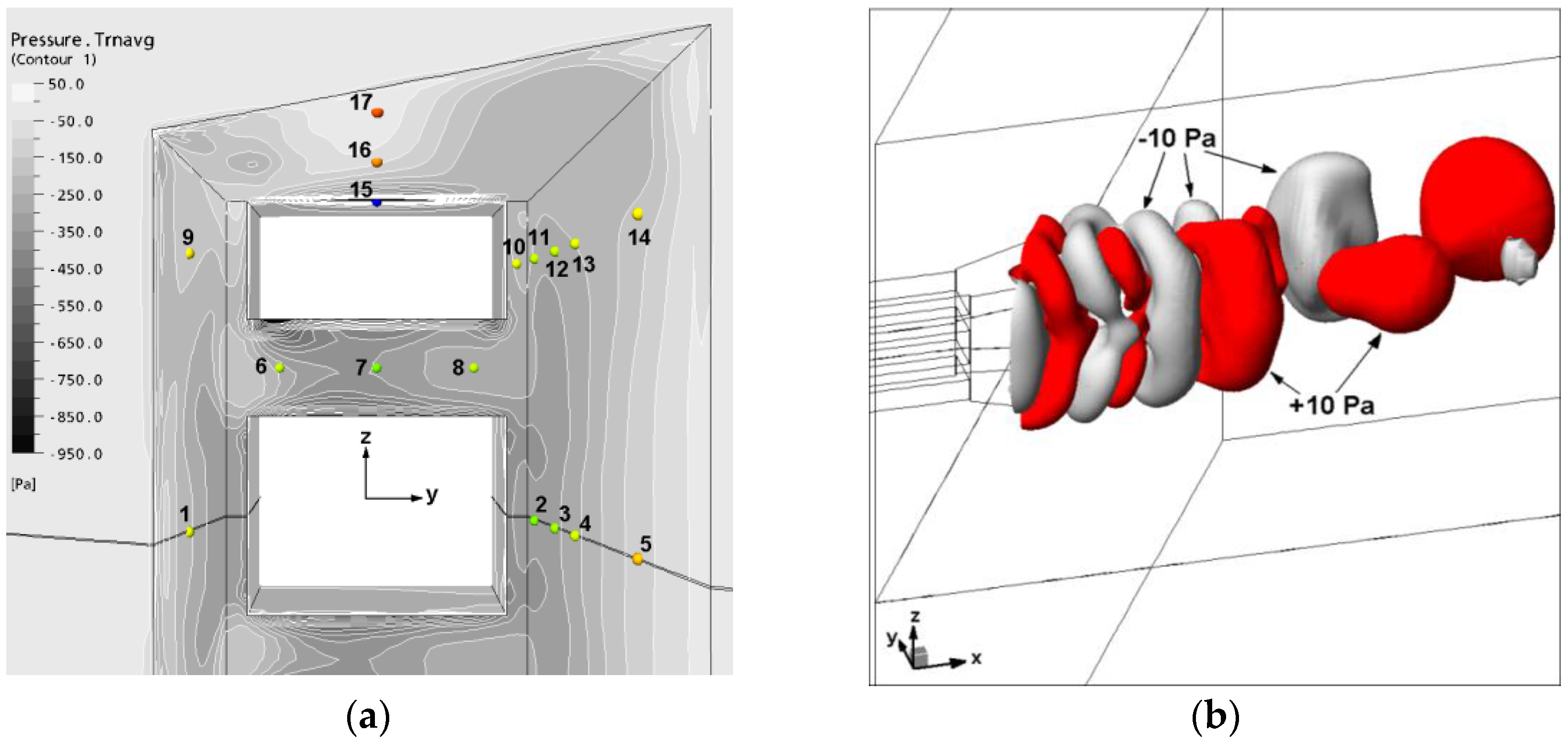
Flow patterns in the recess were expected to be a complex, produced by an arrangement of the inside restructuring of energy in the jet, adversative pressure gradients in the recess and entrainment of fluid from the open atmosphere into the recess. The results of these simulations point to flaws in the nozzle design, which may be avoided in new designs and may also allow the redesign of existing burners to avoid the unfavourable characteristics.

7.1. Pressure Distributions

The recess and multiple-jet system is three-dimensional; however, when viewed on the xy symmetry plane of the primary jet in Figure 6 and the yz plane through the centres of both the primary and secondary jets in Figure 7, the diverging recess is reminiscent of a two-dimensional diffuser, and a description of the flow in these terms aids the understanding of the three-dimensional flow field in general.
The idea of an efficient diffuser, according to [27], is to recover kinetic energy from the mean flow in the form of a rise in pressure, by expanding the duct smoothly to prevent separation of the flow from the walls. The pressure in the diffuser is higher in the centre than on the walls, and this pressure difference results in a force perpendicular to the streamlines directed from the centre outwards, which helps bend the streamlines to follow the diverging walls. An inefficient diffuser is one in which the flow separates as it moves into the diverging section, as this prevents adequate expansion and deceleration of the flow to give the required pressure rise.
The top wall of the recess acted as an efficient diffuser for the secondary jet, which attached smoothly to the upper wall (Figure 2). In moving from the duct to the recess, the flow experienced a step change at the side walls, which induced flow separation similar to the classical backward-facing step problem of fluid mechanics. On the long side of the recess, the primary jet did not attach to the side wall to the same extent as the secondary jet did to the top wall, and there was a reverse flow at the beginning of the recess; however, the primary jet did appear to attach to the long wall to some extent, consistent with the observations given in [26]. On the short side, there was a large reverse flow, and the jet entirely was separated from that wall, also consistent with the observations given in [26].
The pressure distribution in the recess is shown in Figure 8 and Figure 9, where Figure 8 shows pressure on the xy plane through the centre of the primary jet and Figure 9 shows that same plane and the pressure on the recess walls. Some experimentally-measured wall pressures are shown for comparison, and the distribution was qualitatively similar, although the level of accuracy in the measurements is unknown. Any experimental error was compounded by errors in reading data from the original graphs of [26], and as a result, the measurements should be taken as indicative only. Pressure on the geometric centreline of the primary jet was higher than that on the boundaries. The rise in pressure from the start of the recess to the opening at the wall is an adverse pressure gradient. An adverse pressure gradient is required for separation to occur, but does not guarantee it.
Cross-stream pressure drop was sufficient to bend the streamlines towards the long wall, but not the short wall. Although the actual drop in pressure between the start of the recess to the end was the same on each wall, the pressure drop per unit length was lower on the long wall side. Thus, the flow on the long wall side had a low enough pressure drop per unit length and sufficient distance to partially attach to that wall. On the short side, the higher pressure drop per unit length, combined with the shorter length of the wall, prevented the streamlines being diverted sufficiently to attach to this wall. The result of this was separation of the jet from the short wall, which allowed fluid to be drawn into the recess from outside to replace fluid entrained into the jets near the nozzle, aided by the pressure gradient, which was favourable for reverse flow.
Partial attachment of the jet to the long wall and separation from the short wall resulted in the jet being pushed off its geometric axis towards the long wall side (Figure 10). Deviation from the centreline was also seen compared to Geometry B in [15], to a lesser extent, but the mechanisms causing this deviation were entirely different in the present case. As mentioned earlier, there were many three-dimensional factors affecting in the flow pattern in the recess; however, the diffuser analogy has satisfactorily explained what was seen on the axis of symmetry, which was what caused the jets to deviate from their geometric axes.

7.2. Comparison of Different Turbulence Model

Figure 11 shows the velocity decay of the primary jet along the geometric axis. Whereas Perry and Hausler [26] took measurements of the jets in Geometries A and B on the jet centreline, all measurements for Geometry D were made on the geometric axis, because jets in this configuration deviated far more from the centreline, and the angle of deviation varied at different points in the jets, making it impossible to choose a straight line through the centre of the jet.
For the measurement locations along the geometric axis of the primary jet, the standard k-ε model was more accurate than the Reynolds stress model at predicting the centreline velocity decay.
However, these comparisons do not give a true indication of the quality of the predictions because the measurements were not taken on the centreline of the primary jet. To illustrate the reason for this, it is useful to refer to Figure 10, which shows the geometric axes of the jets in black.
The primary jet was expected to deviate towards the long wall, but the extent of this deviation had a large effect on the centreline velocity decay curve. The geometric axis actually cut through the shear layer of the primary jet, and as a result, the decay rate increased with increasing angle of deviation. Had this been an extreme case, were the jet deviated by a large amount, for example 10°, the geometric centreline would cut through the shear layer at an even sharper angle, and the decay rate would have been even larger, even though the actual jet centreline might have decayed at a rate similar to any other jet.

7.3. Velocity Distributions

Velocity profiles in four different planes are shown in Figure 12, Figure 13, Figure 14 and Figure 15 for the Reynolds stress model only. The k-ε model was only used in these predictions to generate an intermediate solution that could be used as an initial guess to stabilise the less robust RSM simulation, and no comparisons are performed. Previous sections have shown that the Reynolds stress model is superior to k-ε for these types of jets, negating the need for comparisons with this model. The planes are: the xy planes through the centre of the primary jet, the secondary jet and the base region separating the primary and secondary jets and also the xz plane through the geometric axes of the primary and secondary jets.
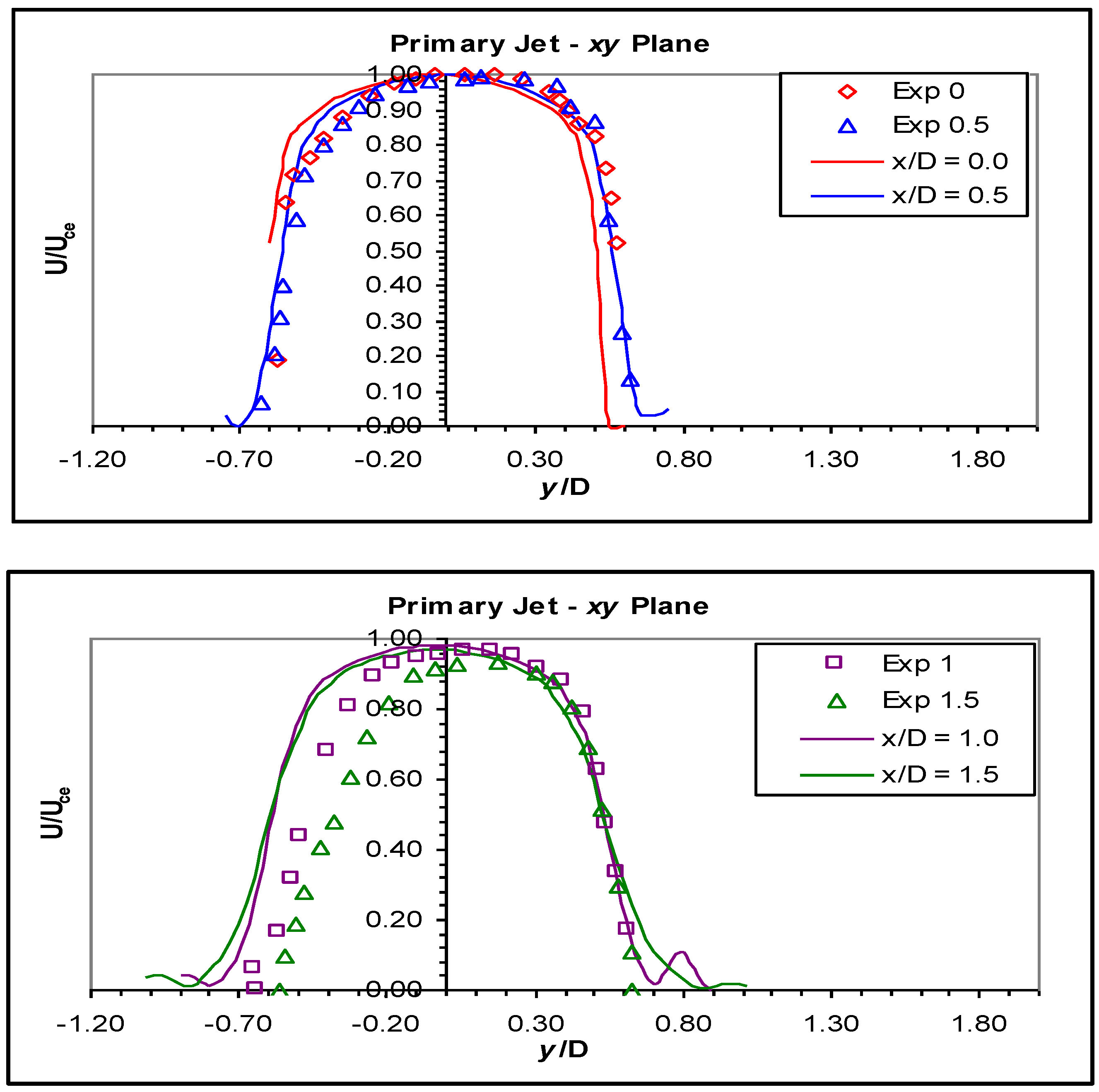
The velocity profiles through the xy plane of the primary jet (Figure 12) show that generally, the CFD model predicted the same qualitative behaviour as observed in the measured jet, but there were deficiencies in the quantitative accuracy of the model. The differences began at the primary jet nozzle, where the calculated profile was fairly symmetric about the geometric axis, but the measured profile was skewed towards the positive y side or the long wall of the recess. At half a diameter from the nozzle, the experimental profile was still skewed, and again, the calculated profile was more symmetric, although at this point, the calculated profile had begun to divert towards the long wall. At one diameter, the CFD model correctly predicted the jet boundary on the long wall side, but the calculated jet was wider on the short wall side than the measurements indicated.
At one and a half diameters, the short side of the jet had reached the open atmosphere, and so, it was only the long side that was still confined by the recess. The long side was well predicted, but the short side boundary of the jet was again too wide and the boundary layer too steep. According to the measured velocity profile, the real jet was pushed across its geometric axis far more than the CFD model predicted at this point. This trend continued as the measurement location moved downstream. Little change occurred between x/D = 1.5 and 2.0. At two diameters, the long wall side of the jet had almost exited the recess. The prediction at two diameters was again reasonable on the long wall side, although the measured shear layer was somewhat steeper than the CFD prediction, but on the short wall side, the predicted profile was still too wide.
At the measurement location three diameters downstream of the nozzle, the jets were no longer bounded or directly influenced by the recess region. From this point onwards, the jets were free jets similar to Geometry B, but with different initial conditions. The jets in Geometry B were well predicted, giving confidence that the free part of the jets in Geometry D would also be well predicted; to the extent they could be given the “wrong” initial conditions at the plane of the wall. The differences in the profiles at three diameters were similar to the previous two locations, with the long side of the jet being in reasonable agreement, while on the short side, the measured jet was thinner and pushed across the geometric axis farther.
At five diameters, the CFD model was still accurate on the long side, predicting the jet boundary well, but the experimental profile had a low highest rate in the middle of the jet and was also thinner than the CFD prediction. Aside from the measured jet being smaller at this point, the locations of the measured and simulated jets were similar, i.e., the movement of the primary jet across its geometric axis was similar in both cases.
At nine diameters, the measured jet had shifted more from the axis, and the velocity profile had become comparatively wider than at five diameters. The model jet moved further off its axis, and the highest velocity also decreased, but not enough to match the measured jet. The changes in the model jet from three, to five and five to nine diameters were similar to the corresponding changes in the experimental jet. It is probable that had the CFD model predicted the flow in the recess better, the profiles downstream of the recess would also have been closer to the measured data.
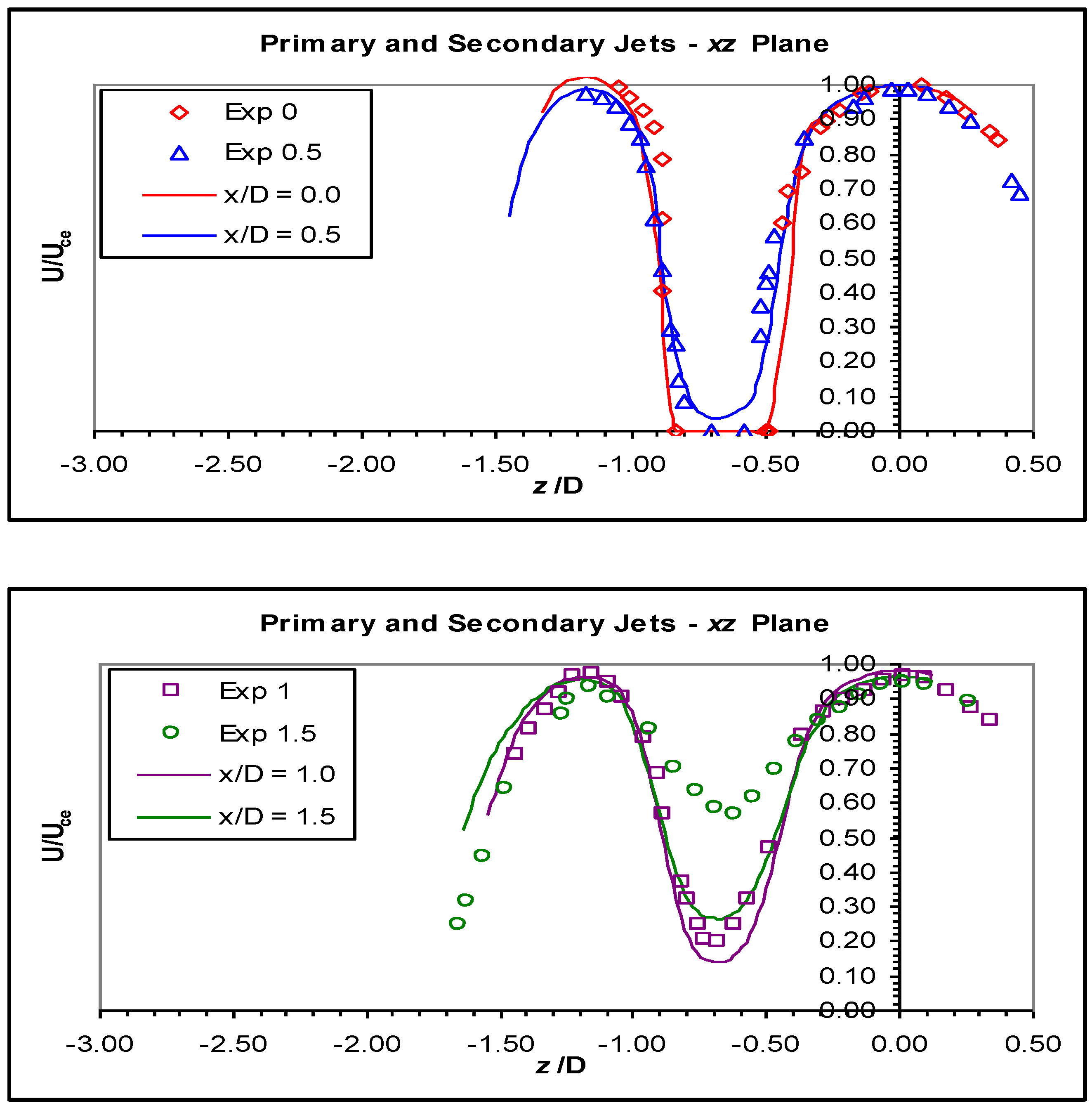
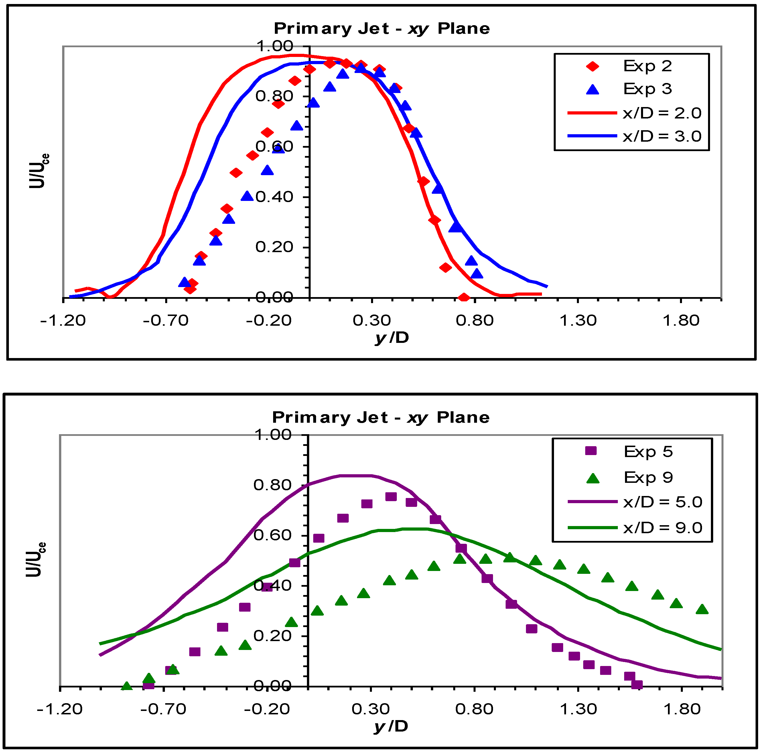
In the xz plane, some confusion existed as to exactly where the measurements were made. Perry and Hausler [26] stated that in the recessed burner, where there was significant movement of the jet towards the long side of the recess, measurements in the xz plane were made on the geometric axis. However, from the xy plane data, the normalised velocities on the axis were approximately 0.5 for x/D = 5 and 0.3 for x/D = 9, but the values on the axis were 0.65 and 0.50, respectively. The latter values matched neither the axis data nor the velocities on the actual jet centreline.
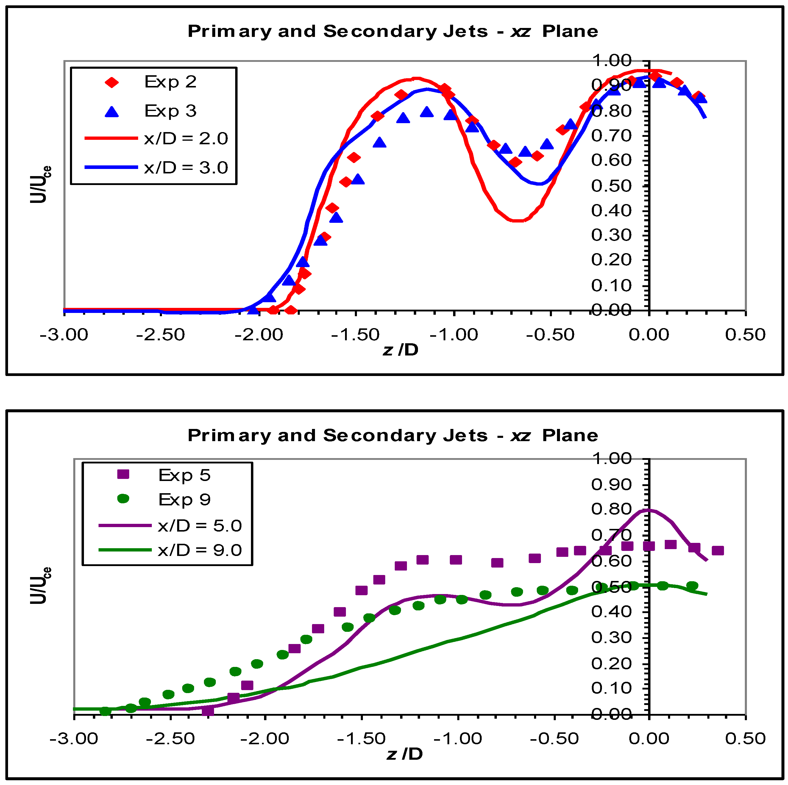
In the xz plane, the CFD model matched the measured data reasonably well in the recess, from x/D = 0 to 1; and even for x/D = 1.5 and 2, the peaks in the primary and secondary jets were predicted well, but the base region between the primary and secondary jets was underpredicted by a significant amount. At three diameters, the model predicted the primary jet well; but the base region was underpredicted, and the secondary jet was overpredicted. The more contentious data at five and nine diameters did not match well; at five diameters, the primary jet peak velocity was too high, and the other parts of the system, the base region and the secondary jet, were too low. At nine diameters, the peak velocity in the primary jet was the same in the model and the experimental data, but again, the base and secondary jet were underpredicted.
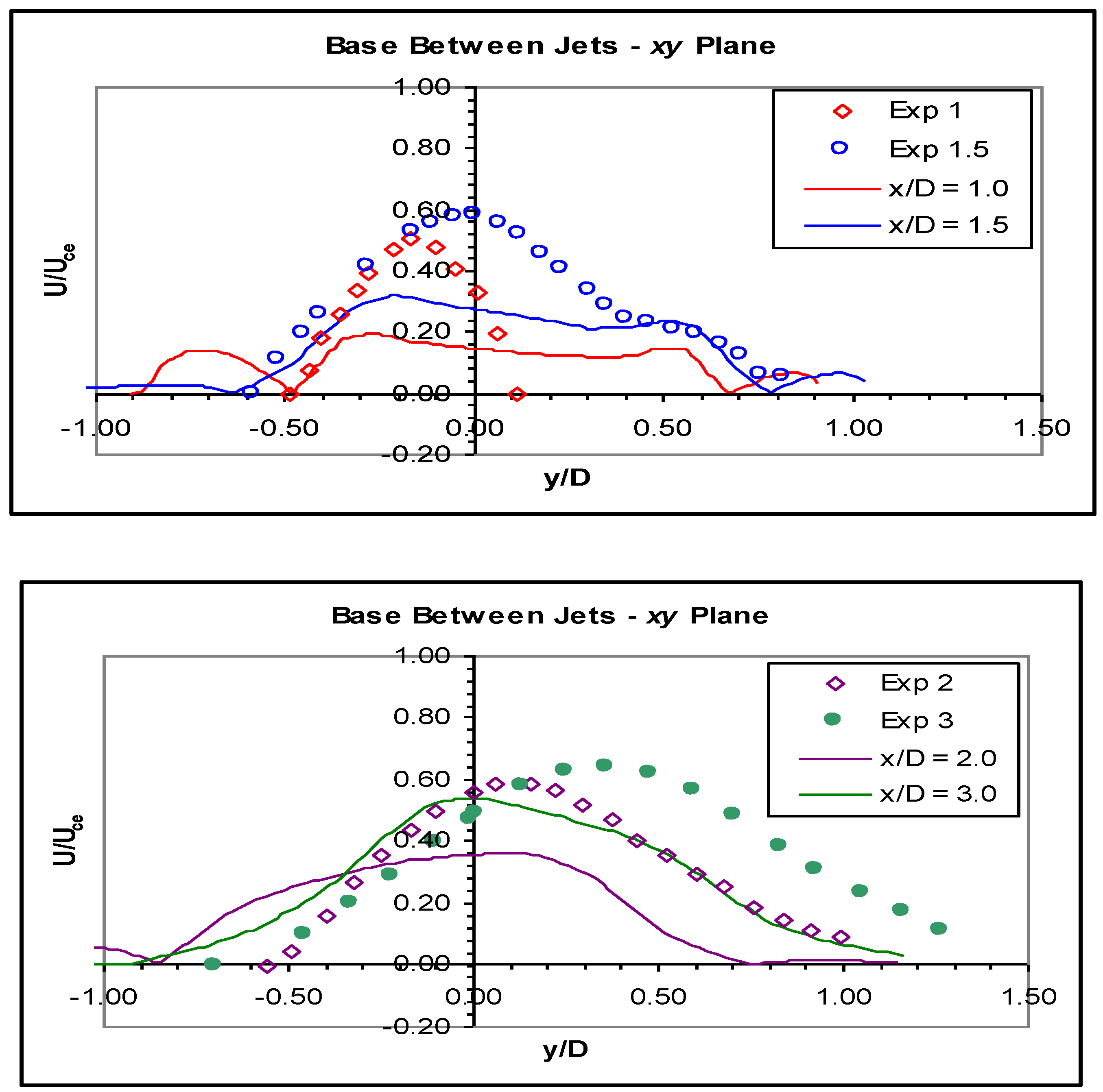
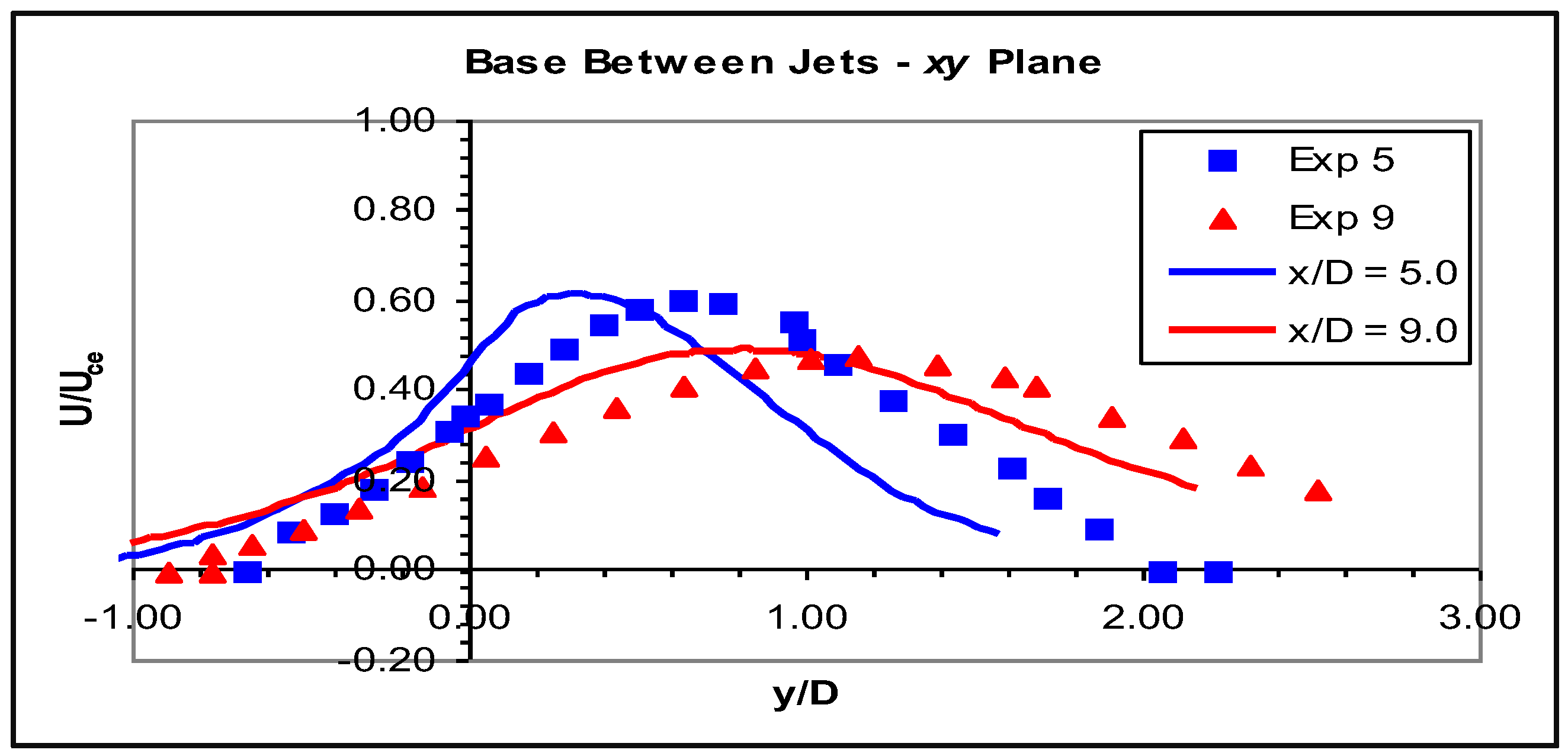
Figure 14 shows the experimental and model profiles in the base region between the jets. The flow development in this region inside the recess was entirely different from the experimental jets. Peaks were found in the experimental profiles near the geometric axis, while the profiles from the simulation were very flat, with almost no peaks visible. The CFD profiles also showed some reverse flows near the recess walls, which were not present in the experimental data. From three diameters onwards, that is the region outside the recess, velocity development in this region was similar in both simulation and experiment. At three diameters, the shape of the profile matched well, although the CFD profile was centred on the axis, whereas the experimental data showed it to be skewed towards the positive y direction, and the peak of the predicted profile was lower. At five diameters, the peak velocity and the shape of the profile matched well between the two sets of data, but again, the experimental jet had deviated further off the geometric axis. A similar situation existed at nine diameters, but the predicted profile was much closer to the measurements than at any other location.
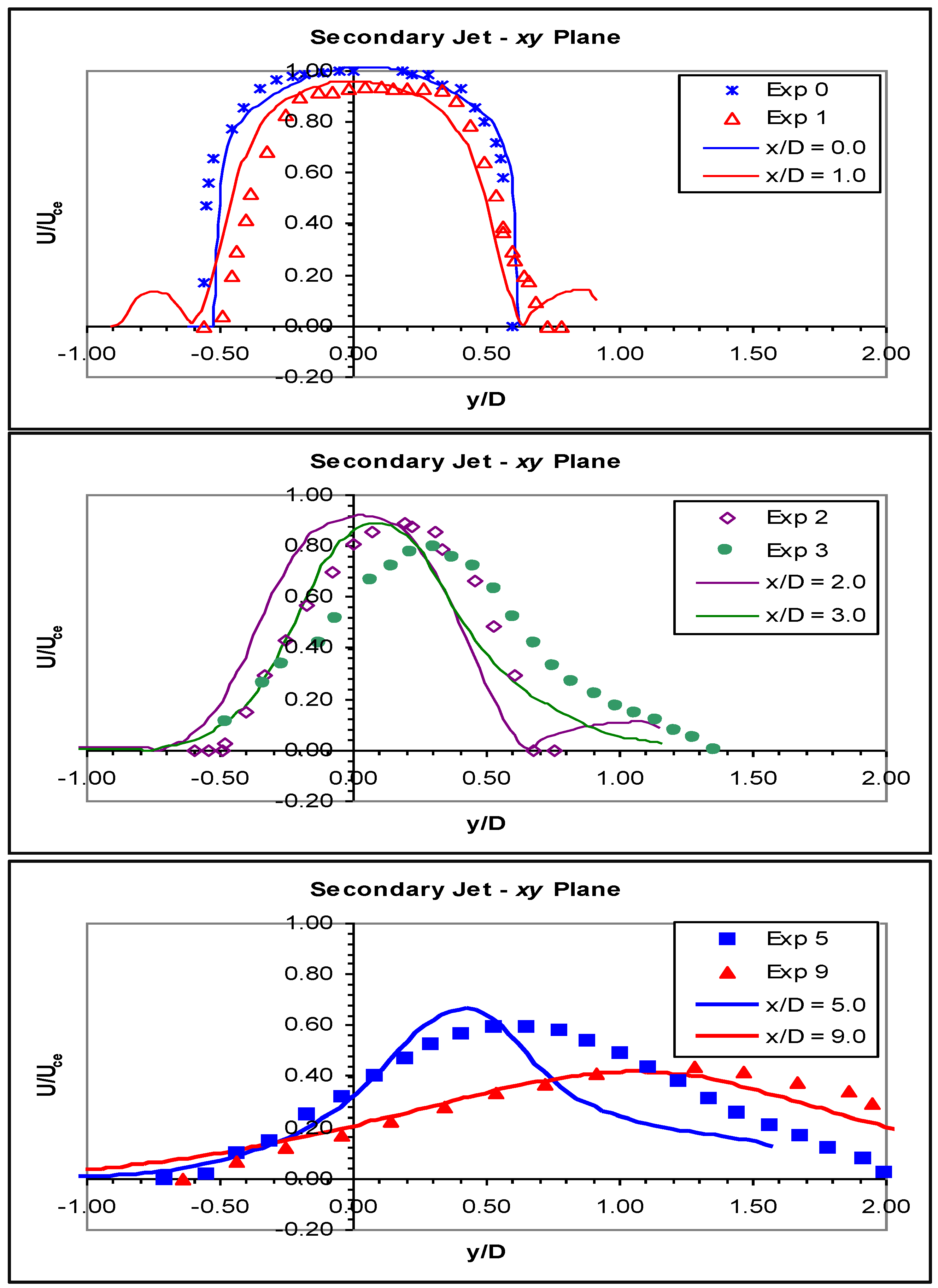
Figure 15 shows the profiles of the secondary jet, which matched the experimental data better than the primary jet profiles. At the nozzle, the CFD model matched the experimental profile well, and at one diameter, this agreement was maintained, although the predicted profile was slightly thinner than the measured one. The experimental data did not show the reverse flow outside of the jet boundary seen in the CFD prediction, because the pitot tube is sensitive to direction and will not sense negative velocities unless oriented correctly.
At x/D = 2, the experimental jet began to deviate from the axis towards the long wall of the recess, and again, the CFD model failed to predict this movement well, although the shape and height of the profile were well matched. At three diameters, the CFD model continued to incorrectly predict the movement of the secondary jet off its geometric axis or as the decay in peak velocity in the jet’s centre.
The decay in peak velocity was recovered at five diameters, the CFD model slightly over predicting the peak of the profile. The jet also moved off its axis by a significant amount, but not enough to match the measured profile. The profile of the simulated jet was narrower than the measured profile, indicating that the CFD model jet had not spread much by this point, but by nine diameters, the model jet had spread almost as much as the experimental jet. The match between the measured data and CFD profile were good at nine diameters, better than in any other plane.
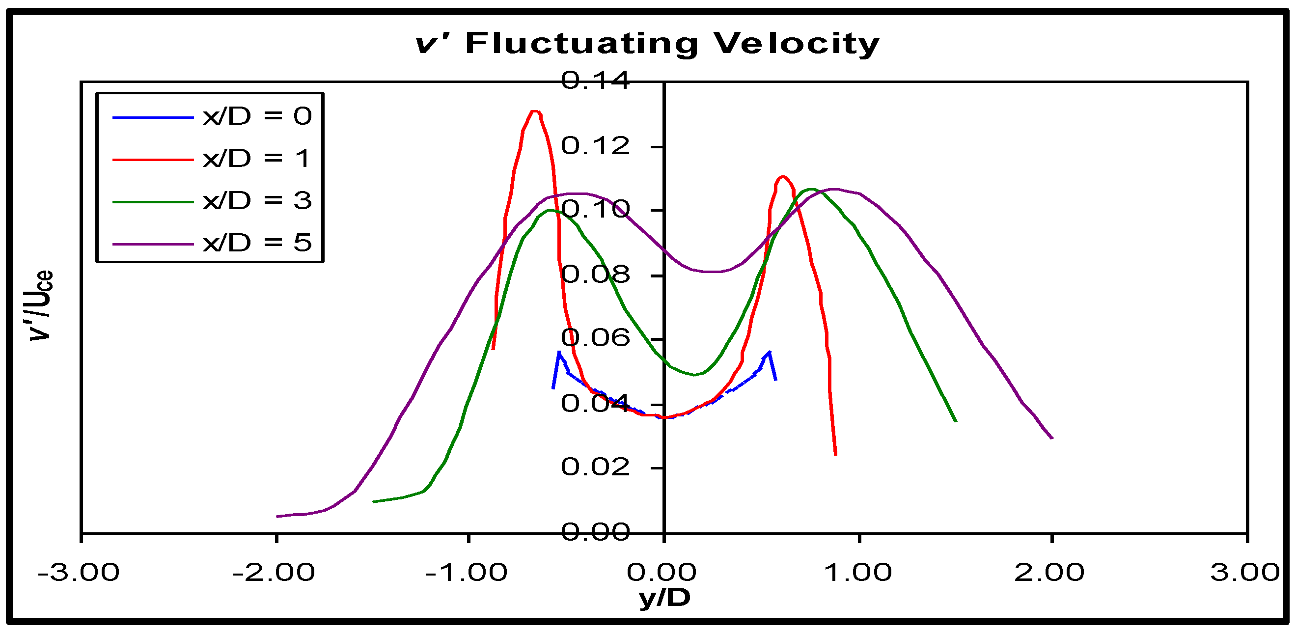
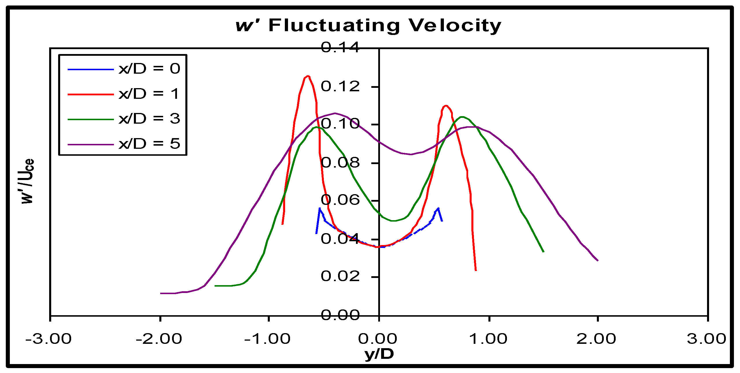
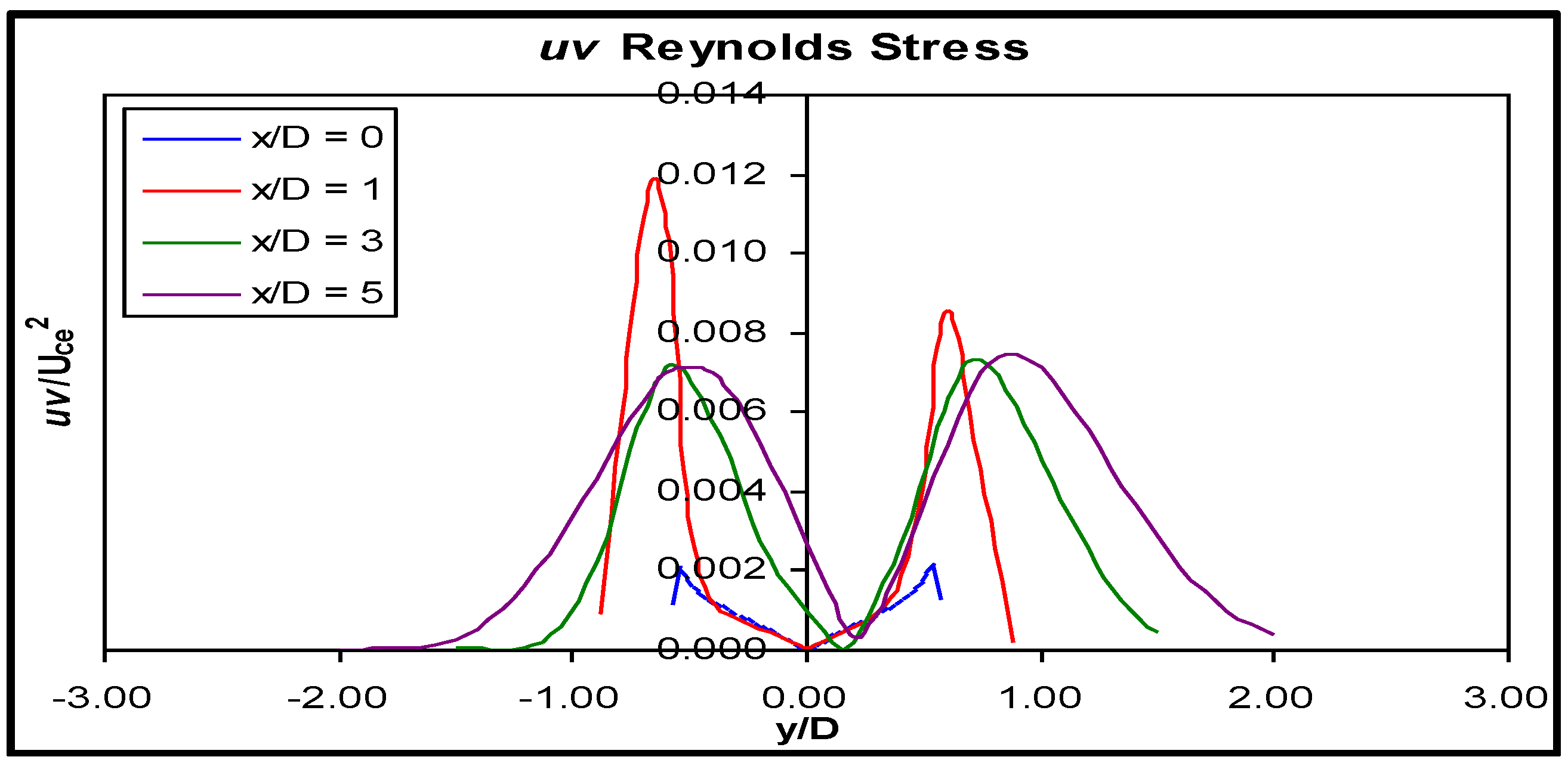
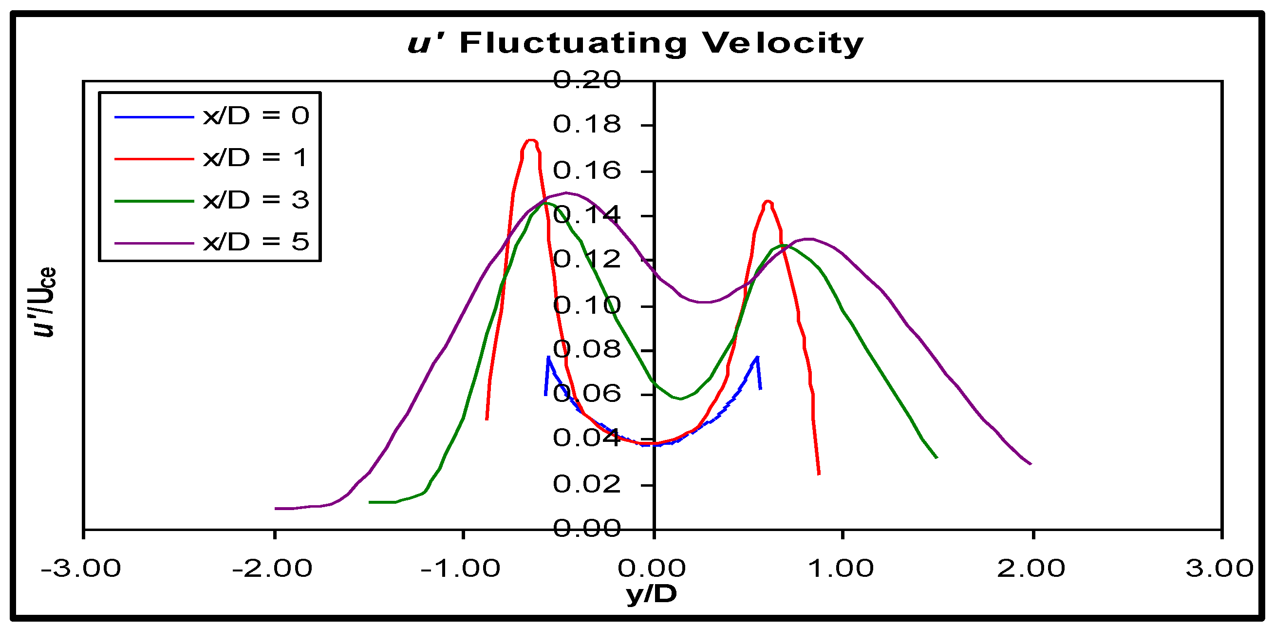
The predicted distribution of turbulent stresses in the xy plane through the centre of the primary jet are shown in Figure 16, Figure 17, Figure 18 and Figure 19, plotted as the fluctuating u’, v’ and w’ velocities normalised to the primary jet centreline exit velocity and the u v ¯ Reynolds stress normalised to the square of that velocity, for consistency with the previous results. No experimentally-measured distributions were available for the selected geometry; comparisons with the Reynolds stress predictions of Geometry B are made.
The inclusion of a recess made a large difference to the distribution of the Reynolds stresses in the primary jet, compared to the distribution in Geometry B [15]. At the burner exit plane, x/D = 0, the profile of u’ was symmetric about the geometric axis because the primary jet nozzle was orthogonal to the local flow direction, unlike Geometry B, where the nozzle was at an angle; refer to Figure 16. The magnitude of u’ at the edges of the nozzle was similar to the long-side of Geometry B at x/D = 0, which was expected, because at this point in Geometry D, the flow was still inside the duct, and the ducts were the same in Geometries B and D. The magnitude of u’ on the centreline was slightly lower in Geometry D, probably due to the nozzle being symmetric, whereas in Geometry B, the short side of the jet had exited the duct before this point and begun interacting with the surrounding fluid, modifying the turbulent fluctuations.
At x/D = 1, the flow was still contained within the recess, but was close to the opening on the short side recess wall; the magnitude of u’ had increased sharply and was now distributed somewhat asymmetrically about the geometric axis. The magnitude on the short wall side of the recess was approximately 15% higher than on the long side of the recess and was located at a position corresponding to the interface of the jet and the reverse flow near the wall. This peak was approximately 20% higher than the corresponding peak in Geometry B. This larger value of u’ and its asymmetric distribution indicated that there was higher shear on the short wall side, an expected result, since there was a reverse flow on the short wall. The difference in magnitude of u’ on each side of the jet was slightly less in Geometry D than in Geometry B. The generation of stress at this position was the highest of any downstream location in Geometry D, indicating that the flow inside the recess had a large effect on the development of the jet outside the recess.
Three diameters downstream of the nozzle, now completely outside the recess, further development of the turbulent fluctuations was qualitatively different from the development of Geometry B, even though they were both free jets. The magnitude of u’ peaked inside the recess due to shear between the jet adjacent fluid and the reverse flow region along the short wall, then dropped once outside. In Geometry B, the magnitude of u’ continued to rise at three diameters, because the shear between the jet and surrounding fluid was still high at this point. In Geometry D, the highest shear was found inside the recess, which prematurely reduced the mean velocity in the jet before it exited to the open atmosphere. The shear between the lower velocity jet and the surrounding fluid outside the recess was therefore less in Geometry D than Geometry B at this point. Between three and five diameters, no further increase in u’ occurred; rather, the peaks reduced as the stress was redistributed within the jet. In Geometry B, the peaks remained the same as the jet moved downstream from this point.
Turbulent fluctuations in the y and z directions, v’ and w’, were very similar to one another, as found in Geometry B. They were found to the approximately 75% of the magnitude of the stream-wise fluctuations, a similar result to Geometry B. At the nozzle, their distributions were slightly asymmetric. The development of v’ and w’ was very similar to the development of u’. Generation was highest inside the recess, and their profiles were again skewed to the short wall side. Upon exiting the recess, there was no new generation of cross-stream normal stress, merely redistribution within the jet.
The u v ¯ stress distribution followed much the same pattern as the normal stresses. The magnitude was low at the duct exit, and the distribution was symmetric about the geometric axis. By x/D = 1, there was a large increase in u v ¯ , much larger than in Geometry B, and the distribution became asymmetric, with the larger peak found on the short wall side. Much like the normal stresses, the u v ¯ shear stress in the primary jet began to reduce substantially upon entering the open atmosphere, and the distributions at three and five diameters were essentially the same, qualitatively different behaviour to that found in Geometry B, where the shear stress continued to increase between one and three diameters, then reduced slightly between three and five diameters.
The primary jet in Geometry B was an angled jet, while the primary jet in Geometry D was an initially orthogonal jet inside a recess, which then exited the recess at an angle to the wall. It is of interest, then, that the turbulent fluctuations of the orthogonal primary jet within the recess were similar to Geometry B, although the fluid dynamics were quite different. The reason for the similarity lies in the asymmetric entrainment of fluid within the jets in the first few diameters after the nozzles in both cases. In Geometry B, the asymmetry was due to one side of the jet exiting the nozzle before the other; in Geometry D, the cause was flow separation from the short, but not the long, wall of the recess. The different mechanisms produced essentially the same development of turbulent stresses, although the magnitudes inside the recess were higher than for the corresponding region in Geometry B.
Once outside the recess, the fluid dynamics were essentially the same in Geometries B and D, but development of the stresses was different, due to the different initial conditions at the exit of the recess. In Geometry D, the velocities at the open end of the recess were lower than in Geometry B, causing less shear between the jet and the surrounding stagnant fluid. This led to less turbulent stress generation outside the recess, with mainly redistribution occurring. In contrast, when the primary jet in Geometry B exited the nozzle at the wall, the velocity was at a maximum, and the shear between the jet and surrounding fluid began to generate large amounts of turbulent stress, which continued for some distance as the jet moved downstream.
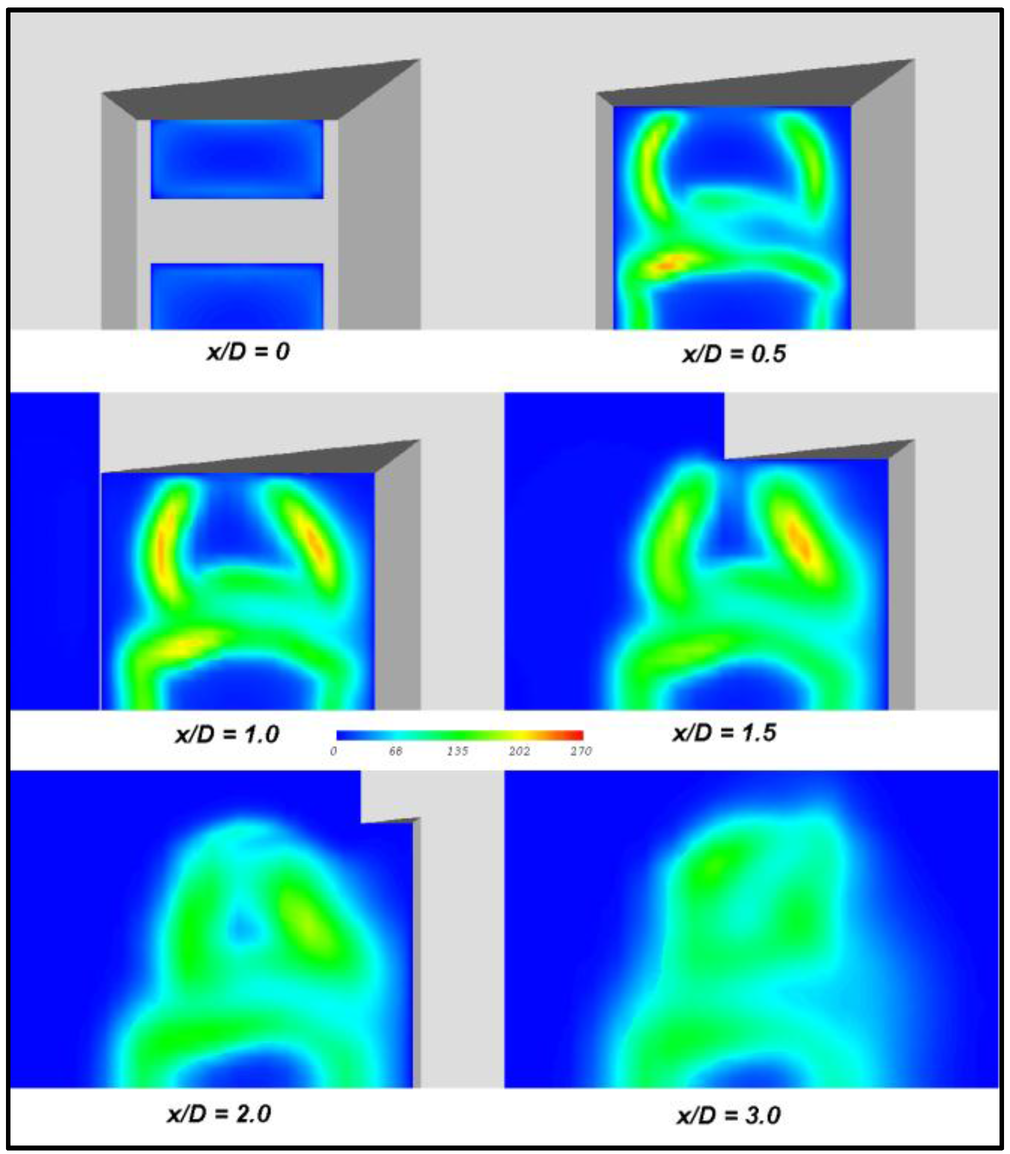
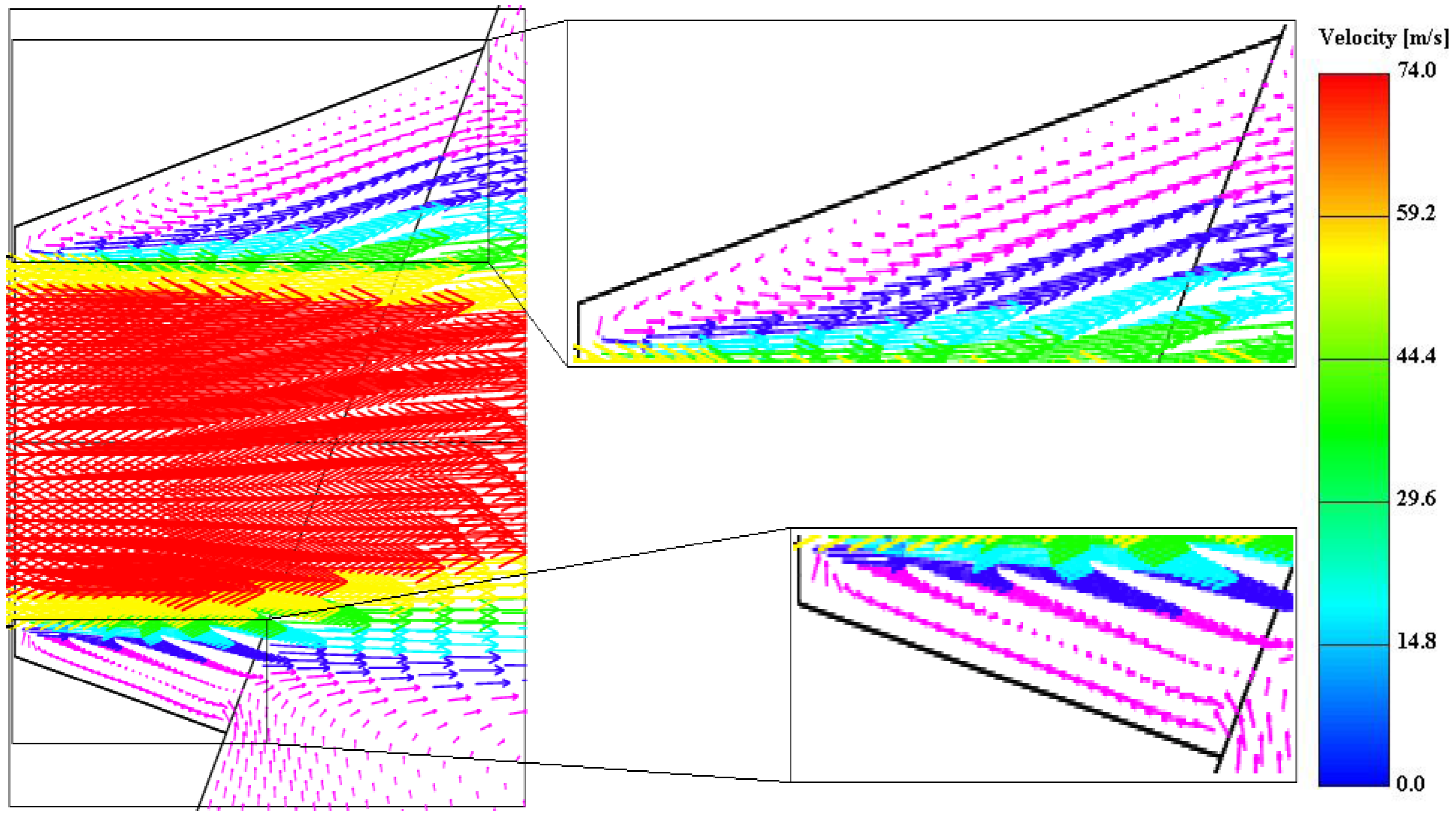
Figure 20 illustrates the development of stream-wise normal stress, u u ¯ , within and just beyond the recess. As the distribution of this stress was typical of each of the Reynolds stresses, only the stream-wise normal stress is shown for illustration.
At x/D = 0.5, peaks in the stream-wise normal stress appeared on the short-side of the recess at the primary and secondary jet boundaries. The magnitude was highest at the primary jet boundary. A region of high turbulent stress appeared around the boundary of both jets, except for the top of the secondary jet, were the turbulent stresses remained minimal. This was due to the lack of a step change from the duct to the top wall of the recess, which allowed the secondary jet to flow smoothly from the duct along the top wall with minimal shear.
By one diameter, the stresses were larger on the short wall side of the recess, due to the reasons mentioned in the preceding paragraphs. Once the jet had exited the recess on that side, the magnitude reduced, while the magnitude of the peak on the long side was maintained until it too exited the recess at x/D > 2. From this point onwards, the peak stress decreased throughout the jet, and the distribution became more homogeneous throughout the two jets, although the centre of the primary jet still contained low levels of turbulence.
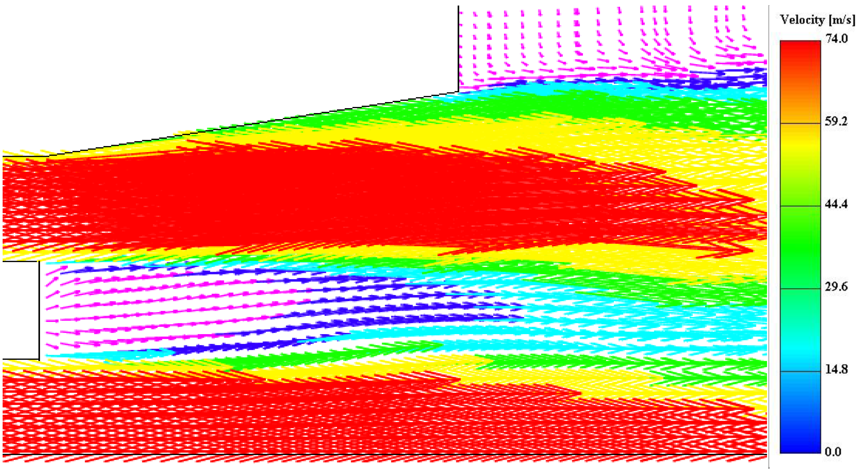
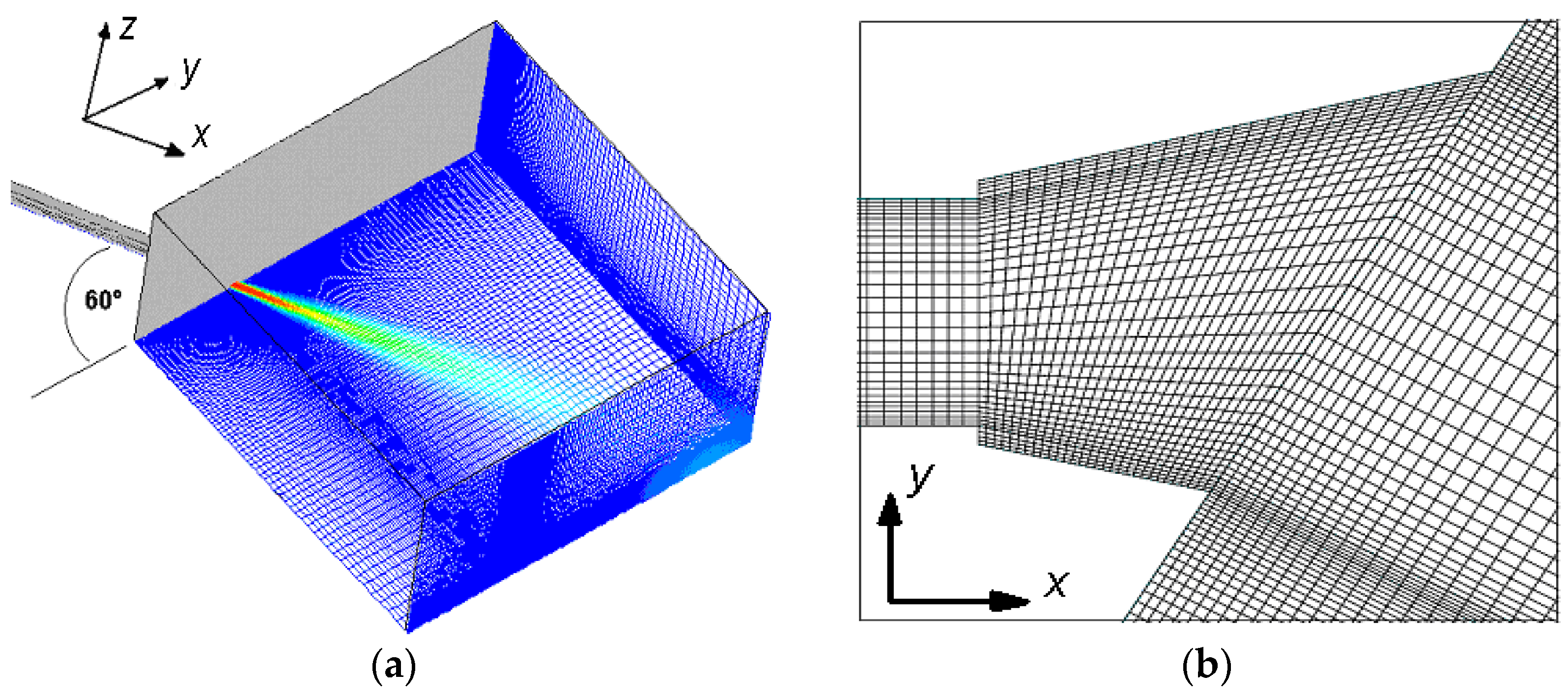
The dynamics of the tri-jet system in the recessed burner geometry were more complex than for the previous two geometries. The recess acted as a diffuser, raising the pressure inside it, creating an adverse pressure gradient in the process. On the long-side the flow was able to partially attach to the recess wall due to bending of the streamlines under cross-stream pressure gradient effects. On the short side, the adverse pressure gradient per unit length was higher, and the length of the wall was too short to allow the flow to attach, resulting in a large reverse flow along the short wall, fed from the outside. The optimum divergence angle for a diffuser is around 6°, while walls of the recess diverged at 10°, and the walls were much shorter than those of a well-designed diffuser, so it is not surprising that the primary jet did not attach to the short wall and maybe a little surprising that it was able to attach to the long wall to the extent that it did.
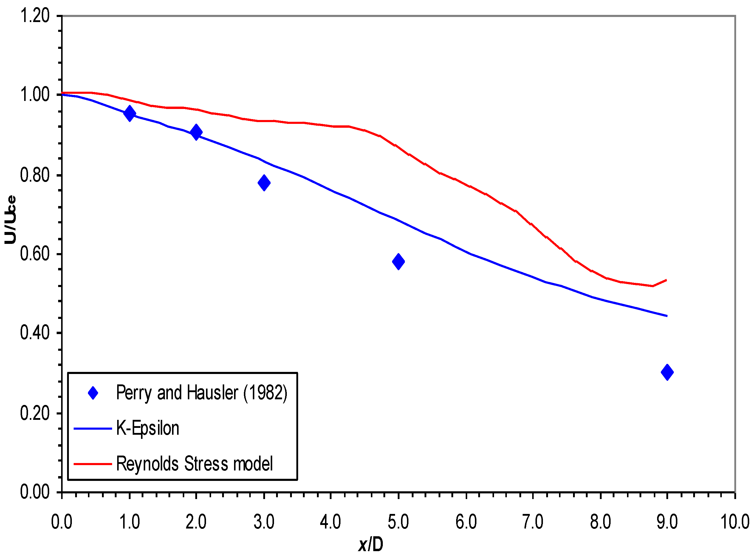
Although the jets did not deflect as far as observed in the experimental model, the mechanism by which this happens has been established in [26] and confirmed and elucidated by the current results. Bearing in mind that the decay rate of the centreline velocities presented in the results for Geometry D was along the geometric axis and that the decay rate would be lower on the actual jet axis, the decay in velocity was still larger than for either Geometry A or B, as a result of the loss of momentum in the recess.
The CFD model predicted the burner behaviour reasonably well on the long wall side of the recess, but consistently over-predicted the jet width on the short wall side. Recirculation on the short side of the recess in the [26] physical model was larger than in the CFD model. This indicated that the calculated did not handle the adverse pressure gradient well, as is well known for wall function treatments, and a low Reynolds number model that integrates the velocity to the wall may perform better.

8. Conclusions

CFD modelling of recessed burner’s jets in a tangentially-fired furnace was conducted. There was a significant increase in the decay rate of velocity along the jet centrelines, compared to the other two geometries. Assuming that the characteristics of these jets are indicative of what may be expected of jets from a real recessed burner oriented at a similar angle to the furnace wall, the latter would reach the fireball in the central region of the furnace with less momentum than jets from non-recessed nozzles. Furthermore, they would move further from their geometric axes than non-recessed jets. These two characteristics are likely to have adverse effects. Firstly, the jets from geometrically-similar burners may not have enough momentum to sustain the swirl in the centre of the furnace, a requirement for a stable and intense fireball; secondly, movement of the jet from its axis may result in an incorrect trajectory with respect to the firing circle in the centre, which would also affect the fireball; and finally, the jets may never even make it to the centre of the furnace, due to the large-scale circulation in the furnace, causing the jet to deviate even further, with the possibility of impinging on the wall, something that was reported to have occurred in boiler Units 3 and 4 at Yallourn W power station. The current results show that the nozzle has a significant effect on the development of jets. The particular design of the nozzle, i.e., straight or angled, flush or recessed, has considerable influence on the characteristics of jets. Computational fluid dynamics using conventional turbulence model closures has been shown to be an effective tool for predicting the mean-flow characteristics of jets from such nozzles. CFD also provides the scope to investigate new nozzle designs, which could produce jets with more favourable near-field characteristics for brown coal boilers. In designing new nozzles, it would be helpful to understand exactly what physical mechanisms are responsible for entrainment and jet development, which is the focus of our future work.

Acknowledgments

The authors gratefully acknowledge the financial received for this research from the Cooperative Research Centre (CRC) for Clean Power from Lignite, which is established and supported under the Australian Government’s Cooperative Research Centre program. The authors would to like to acknowledge the financial and other support of Swinburne University of Technology.

Author Contributions

James T. Hart and Jamal Naser designed and modelled the geometry and setup; Peter J. Witt and Jamal Naser developed the concept and contributed to analysis methodology; James T. Hart analyse the data; Md. Rezwanul Karim and Arafat Ahmed Bhuiyan wrote the paper.

Conflicts of Interest

The authors declare no conflict of interest

References

  1. Kenbar, A.M.A.; Beltagui, S.A.; Maccallum, N.R.L. Combustion aerodynamics of a gas-fired furnace with peripheral fuel injection. Exp. Therm. Fluid Sci. 1995, 10, 335–346. [Google Scholar] [CrossRef]
  2. Bhuiyan, A.A.; Naser, J. Effect of recycled ratio on heat transfer performance of coal combustion in a 0.5MWth combustion test facility. In proceeding of 19th Australasian Fluid Mechanics Conference, Melbourne, Australia, 8–11 December 2014.
  3. Bhuiyan, A.A.; Naser, J. Numerical modelling of oxy fuel combustion, the effect of radiative and convective heat transfer and burnout. Fuel 2015, 139, 268–284. [Google Scholar] [CrossRef]
  4. Bhuiyan, A.A.; Naser, J. Computational modelling of co-firing of biomass with coal under oxy-fuel condition in a small scale furnace. Fuel 2015, 143, 455–466. [Google Scholar] [CrossRef]
  5. Bhuiyan, A.A.; Naser, J. Numerical modeling of biomass co-combustion with pulverized coal in a small scale furnace. Procedia Eng. 2015, 105, 504–511. [Google Scholar] [CrossRef]
  6. Luo, R.; Zhang, Y.; Li, N.; Zhou, Q.; Sun, P. Experimental study on flow and combustion characteristic of a novel swirling burner based on dual register structure for pulverized coal combustion. Exp. Therm. Fluid Sci. 2014, 54, 136–150. [Google Scholar] [CrossRef]
  7. Biagioli, F.; Güthe, F.; Schuermans, B. Combustion dynamics linked to flame behaviour in a partially premixed swirled industrial burner. Exp. Therm. Fluid Sci. 2008, 32, 1344–1353. [Google Scholar] [CrossRef]
  8. Bhuiyan, A.A.; Naser, J. Thermal characterization of coal/straw combustion under air/oxy-fuel conditions in a swirl-stabilized furnace: A CFD modelling. Appl. Therm. Eng. 2016, 93, 639–651. [Google Scholar] [CrossRef]
  9. Bhuiyan, A.A.; Naser, J. CFD modelling of co-firing of biomass with coal under oxy-fuel combustion in a large scale power plant. Fuel 2015, 159, 150–168. [Google Scholar] [CrossRef]
  10. Bhuiyan, A.A.; Naser, J. A CFD modelling of radiative performance in co-firing of biomass with victorian brown coal in industrial furnace. In Proceeding of Eleventh International Conference on CFD in the Minerals and Process Industries CSIRO, Melbourne, Australia, 7–9 December 2015.
  11. Al-Abbas, A.H.; Naser, J. Computational fluid dynamic modelling of a 550 MW tangentially-fired furnace under different operating conditions. Procedia Eng. 2013, 56, 387–392. [Google Scholar] [CrossRef]
  12. Al-Abbas, A.H.; Naser, J.; Dodds, D. CFD modelling of air-fired and oxy-fuel combustion in a large-scale furnace at Loy Yang A brown coal power station. Fuel 2012, 102, 646–665. [Google Scholar] [CrossRef]
  13. Ahmed, S.; Hart, J.; Nikolov, J.; Solnordal, C.; Yang, W.; Naser, J. Investigation of aerodynamics of a recessed rectangular slot-burner used in tangentially-fired furnaces by varying jet velocity ratio in the presence of cross-flow. Exp. Therm. Fluid Sci. 2015, 68, 109–122. [Google Scholar] [CrossRef]
  14. Ahmed, S.; Hart, J.; Nikolov, J.; Solnordal, C.; Yang, W.; Naser, J. The effect of jet velocity ratio on aerodynamics of a rectangular slot-burner in the presence of cross-flow. Exp. Therm. Fluid Sci. 2007, 32, 362–374. [Google Scholar] [CrossRef]
  15. Hart, J.T.; Naser, J.A.; Witt, P.J. Aerodynamics of an isolated slot-burner from a tangentially-fired boiler. Appl. Math. Model. 2009, 33, 3756–3767. [Google Scholar] [CrossRef]
  16. Bhuiyan, A.A.; Islam, A.S.; Amin, M.R. Numerical prediction of laminar characteristics of fluid flow and heat transfer in finned-tube heat exchangers. Innov. Syst. Des. Eng. 2011, 2, 1–12. [Google Scholar]
  17. Bhuiyan, A.; Islam, A.; Amin, M. Numerical study of 3D thermal and hydraulic characteristics of wavy fin-and-tube heat exchanger. Front. Heat Mass Transfer 2012, 3. [Google Scholar] [CrossRef]
  18. Bhuiyan, A.A.; Amin, M.R.; Islam, A.S. Three-dimensional performance analysis of plain fin tube heat exchangers in transitional regime. Appl. Therm. Eng. 2013, 50, 445–454. [Google Scholar] [CrossRef]
  19. Bhuiyan, A.A.; Amin, M.R.; Naser, J.; Islam, A.K.M.S. Effects of geometric parameters for wavy finned-tube heat exchanger in turbulent flow: A CFD modelling. Front. Heat Mass Transfer 2015, 6. [Google Scholar] [CrossRef]
  20. Jones, W.; Launder, B. The prediction of laminarization with a two-equation model of turbulence. Int. J. Heat Mass Transfer 1972, 15, 301–314. [Google Scholar] [CrossRef]
  21. Yakhot, V.; Orszag, S.A. Renormalization group analysis of turbulence. I. Basic theory. J. Sci. Comput. 1986, 1, 3–51. [Google Scholar] [CrossRef] [PubMed]
  22. Launder, B.; Reece, G.J.; Rodi, W. Progress in the development of a Reynolds-stress turbulence closure. J. Fluid Mech. 1975, 68, 537–566. [Google Scholar] [CrossRef]
  23. Launder, B.E.; Spalding, D. The numerical computation of turbulent flows. Comput. Methods Appl. Mech. Eng. 1974, 3, 269–289. [Google Scholar] [CrossRef]
  24. Patankar, S. Numerical Heat Transfer and Fluid Flow; CRC Press: Boca Raton, FL, USA, 1980. [Google Scholar]
  25. Rhie, C.-M. Numerical Study of the Flow Past an Isolated Airfoil with Separation. Ph.D. Thesis, University of Illinois, Urbana-Champaign, IL, USA, 1982. [Google Scholar]
  26. Perry, J.; Hausler, T. Aerodynamics of Burner Jets Designed for Brown Coal Fired Boilers–Part. IV; Report/State Electricity Commission of Victoria, Research and Development Department: Victoria, Australia, 1984. [Google Scholar]
  27. Massey, B. Mechanics of Fluids; Stanley Thornes Publishers Ltd.: London, UK, 1998. [Google Scholar]
Figure 1. Schematic of a boiler indicating the firing circle of the burner jets.
Fluids 01 00010 g001
Figure 2. Experimental burner configurations. (a) Layout; (b) Burner specifications.
Fluids 01 00010 g002
Figure 3. Body-fitted mesh Geometry D recess. (a) 3D view; (b) 2D inlet view.
Fluids 01 00010 g003
Figure 4. Velocity profiles in the xy and xz planes for grid sensitivity.
Fluids 01 00010 g004
Figure 5. Flow pattern in the recess of Geometry D.
Fluids 01 00010 g005
Figure 6. Velocity vectors in the xy plane through the centre of the primary jet.
Fluids 01 00010 g006
Figure 7. Velocity vectors in the vertical plane of the primary and secondary jet.
Fluids 01 00010 g007
Figure 8. Pressure distribution on the symmetry plane. (a) mean pressure; (b) instantaneous pressure.
Fluids 01 00010 g008
Figure 9. Mean wall static pressure distribution in (a) the recess and (b) iso-surface of instantaneous positive and negative pressure.
Fluids 01 00010 g009
Figure 10. Potential cores (0.8 UCE) and velocity distributions in the xy plane at z = 0.
Fluids 01 00010 g010
Figure 11. Geometric axis velocity decay for the primary jet.
Fluids 01 00010 g011
Figure 12. Velocity profiles in the xy plane for the primary jet for the Reynolds Stress Model (RSM).
Fluids 01 00010 g012aFluids 01 00010 g012b
Figure 13. Velocity profiles in the xz plane for the primary and secondary jets for the RSM.
Fluids 01 00010 g013aFluids 01 00010 g013b
Figure 14. Velocity profiles in the xy plane for the base between jets for the RSM.
Fluids 01 00010 g014aFluids 01 00010 g014b
Figure 15. Velocity profiles in the xy plane for the secondary jet for the RSM.
Fluids 01 00010 g015
Figure 16. u' fluctuating velocity distribution in the xy plane through the primary jet.
Fluids 01 00010 g016
Figure 17. v' fluctuating velocity distribution in the xy plane through the primary jet.
Fluids 01 00010 g017
Figure 18. w' fluctuating velocity distribution in the xy plane through the primary jet.
Fluids 01 00010 g018
Figure 19. uv Reynolds stress distribution in the xy plane through the primary jet.
Fluids 01 00010 g019
Figure 20. Development of the u u ¯ stress distribution.
Fluids 01 00010 g020
Table 1. Description of experimental burner configurations.
NameDescription
Geometry AA nearly square primary jet flanked above and below by rectangular secondary jets, discharging orthogonally from a wall into a large room.
Geometry BSame as Geometry A, but the jets make an angle of 60° to the wall.
Geometry CSame as Geometry B, but with jets discharging into a straight-walled recess before exiting into the open atmosphere.
Geometry DSame as Geometry C, but with a diverging recess. This was geometrically similar to the recessed burner used in the furnace.
Table 2. Comparison of Yallourn and physical/CFD model nozzles.
PropertyYallourn NozzleModel Nozzle
Primary jet
Reynolds number4.6 × 1051.3 × 105
Slot width1020 mm37.5 mm
Height800 mm29.0 mm
Gas velocity39.2 m·s−160 m·s−1
Secondary jet
Reynolds number3.8 × 1059.3 × 104
Slot width1020 mm37.5 mm
Height565 mm17.0 mm
Gas velocity32.5 m·s−160 m·s−1
Base between jets
Base height1020 mm37.5 mm
Width380 mm14.0 mm

