Measuring and Calculating Current Atmospheric Phosphorous and Nitrogen Loadings to Utah Lake Using Field Samples and Geostatistical Analysis

Abstract

Atmospheric nutrient loading through wet and dry deposition is one of the least understood, yet can be one of the most important, pathways of nutrient transport into lakes and reservoirs. Nutrients, specifically phosphorus and nitrogen, are essential for aquatic life but in excess can cause accelerated algae growth and eutrophication and can be a major factor that causes harmful algal blooms (HABs) that occur in lakes and reservoirs. Utah Lake is subject to eutrophication and HABs. It is susceptible to atmospheric deposition due to its large surface area to volume ratio, high phosphorous levels in local soils, and proximity to Great Basin dust sources. In this study we collected and analyzed eight months of atmospheric deposition data from five locations near Utah Lake. Our data showed that atmospheric deposition to Utah Lake over the 8-month period was between 8 to 350 Mg (metric tonne) of total phosphorus and 46 to 460 Mg of dissolved inorganic nitrogen. This large range is based on which samples were used in the estimate with the larger numbers including results from “contaminated samples”. These nutrient loading values are significant for Utah Lake in that it has been estimated that only about 17 Mg year⁻¹ of phosphorus and about 200 Mg year⁻¹ of nitrogen are needed to support a eutrophic level of algal growth. We found that atmospheric deposition is a major contributor to the eutrophic nutrient load of Utah Lake.

1. Introduction

1.1. Study Goals and Importance

Nutrients have been the focus of considerable scientific research in relation to eutrophication and also the growth of harmful algal blooms (HABs) [1,2]. Nutrients can enter an aquatic ecosystem in a variety of ways: surface tributaries, storm and wastewater discharges, groundwater, and from the atmosphere. Of these different avenues, atmospheric deposition is commonly neglected during the formation of a nutrient budget as in most areas it is not considered a significant source. Recently, with the increased focus on eutrophication of water bodies by nitrogen (N) and phosphorus (P), studies have found that atmospheric deposition is an important part of the total nutrient budget for many aquatic ecosystems [3,4,5,6].

Shallow lakes such as Utah Lake might be even more susceptible to atmospheric deposition because of their large surface area to volume ratios. Despite these characteristics, atmospheric deposition is commonly neglected with respect to the nutrient budgets of Utah Lake [7]. The objective of this work is to: (1) quantify the atmospheric loading of total phosphorous (TP) and dissolved inorganic nitrogen (DIN) to Utah Lake, (2) evaluate the spatial variability of TP and DIN loads over the surface of Utah Lake, and (3) characterize the temporal variability of TP and DIN loads among seasons.

This case study is important as it clearly demonstrates, with field-sample data, the importance and magnitude of atmospheric nutrient loadings. For Utah Lake, and we suspect for many other lakes and reservoirs, reducing nutrient loads from other sources may be costly and because atmospheric loads were neglected, may not produce the expected results. In the case of Utah Lake, we show that atmospheric loads can support a eutrophic level of algae growth.

1.2. Utah Lake Water Quality Background

There is increased interest recently in nutrient loadings to Utah Lake [8]. There is a controversy about the cost and effectiveness of reducing the large nutrient loadings from waste water treatment plants (WTTPs). There is agreement that the WTTPs contribute significant loads to Utah Lake, but there is disagreement on whether reducing or even eliminating these loads would significantly affect algal growth in Utah Lake. Currently phosphorous is not a limiting nutrient in Utah Lake and is present in excess. The debate is whether reducing WTTP TP loadings would be sufficient to reduce phosphorus loads such that they could be limiting to overall algal growth, as well as to limit HABs [7,8,9]. Many well-understood factors can be limiting for excessive algal growth and the occurrence of HABs. These include light levels, water clarity, water temperatures, slow-moving or stagnant waters, and high nutrient levels [10,11,12]. Of these factors, only nutrients can usually be controlled. In Utah Lake many of these factors affect algal growth and depending on climatology and seasonal effects can be limiting [13,14]. For example, at certain times of the year, light penetration (Secchi depth measurements of only a few centimeters) can be so low as to be a limiting factor in algal growth [7,8,15,16,17].

In 2004, Utah Lake was listed on Utah’s §303(d) list for exceedance of state criteria for total phosphorus (TP) and total dissolved solids (TDS) concentrations. The State of Utah’s Division of Water Quality conducted a study to calculate total phosphorus loadings to Utah Lake. The sources that were included in this study were tributaries (including WWTPs), groundwater, springs, and miscellaneous surface flows. Of the total phosphorus loading, the tributaries were found to contribute 97.2% [7]. Atmospheric deposition was not considered, mainly because little to no information was available. Since that time, Abu-Hmeidan, Williams and Miller [15] found that historic sediments in the lake have high phosphorous concentrations that affect water quality. Laboratory tests showed that Utah Lake sediments can contribute anywhere between 0.24 to 19 mg/L of TP to water in laboratory columns. This study also showed that soils on the Utah Lake shore are historic sediments that have high phosphorous values, up to 1000 mg/kg with average values over 700 mg/kg [15].

Merritt and Miller [9] completed an extensive eutrophic and nutrient loading evaluation for Utah Lake. They confirmed TP loadings from the earlier analysis by the Utah Department of Water Quality (DWQ) and studies by the engineering firm Psomas based on water inflows. They evaluated the impact of these loadings using the Larsen and Mercier Trophic State Model and the Carlson Trophic State Index Model [18,19]. They concluded that the actual lake state is currently moderately eutrophic, but P and N loadings estimated from water inflows to the lake are some 15 to 20 times larger than needed to support a eutrophic level of algal growth. They also found that for these estimated loadings, the N/P ratio was approximately 8, which indicates that nitrogen would be more limiting than P if nutrients are the limiting factor. They noted that this may have some impact, though tenuous, on the presence of HABs in the lake at times. Overall, Merritt and Miller [9] concluded that phosphorus and nitrogen loadings from water inflows could not be reduced sufficiently to make nutrients the limiting factors to algal growth. They reported that light limitation, via the high natural turbidity of the lake, was likely the overall limiting factor. They recommended quantification of atmospheric nutrient deposition to better understand the feasibility of nutrient control studies and make these studies more accurate. These recommendations were submitted before recent research that indicates that lake sediments may also be a large nutrient source to Utah Lake [15]. Based on the Larsen–Mercier Model, they concluded that only 17 Mg (tons) year⁻¹ of phosphorus was needed to support the current moderately eutrophic state of the lake (Note on units, English tons from previous studies have been directly converted to Metric tonnes (Mg) which is 1000 kg. This was done to maintain significant figures as the nutrient estimates have significant uncertainty and a more precise conversion would have resulting in numbers with higher precision than is warranted by the data). Using a N/P ratio of 12 for the algae, this means about 200 Mg (tons) year⁻¹ of nitrogen would be needed by Utah Lake algae. Current estimated nutrient loadings are much higher than this, even without considering atmospheric deposition or sediment sources, and Merritt and Miller [9] noted it would not be feasible to reduce nutrient loadings to this level by improving WWTP effluent concentrations.

1.3. Deposition Clssification and Collection

The National Atmospheric Deposition Program (NADP), the primary atmospheric deposition monitoring program in the United States, does not measure TP in precipitation samples. As a result, little data are available for atmospheric deposition of TP in Utah. However, there have been several studies performed in the Western United States with regard to nitrogen deposition. In these studies, nitrate deposition in the Utah Wasatch Front produced concentrations as high as 2.0 kg/ha N [20].

There are three main classifications of atmospheric deposition: bulk deposition, wet deposition, and dry deposition. Bulk deposition has been the most common form of atmospheric collection for decades [21,22]. Recently, it has become increasingly common to collect both wet and dry deposition. Wet deposition is defined as the process by which atmospheric pollutants become associated with cloud or precipitation droplets (or particles) and subsequently delivered to the earth’s surface during precipitation. Dry deposition is the process whereby gases and aerosols are deposited directly from the atmosphere to surfaces. Dry deposition sources principally include particulates from the burning of fossil fuels, forest fires, wind erosion of soil, aerosols from agricultural practices, and plant pollen [3,4,23].

Sampling devices used in the collection of atmospheric deposition vary, depending on the type of deposition to be measured. It is common for researches to collect samples using wet–dry samplers. In these samplers, both wet and dry deposition samples are collected using two buckets and a moisture sensor. The bucket corresponding to either wet or dry deposition is left open to the atmosphere depending on whether wet deposition or dry deposition is being collected. The moisture sensor is used to close one bucket and open the other when conditions change [24].

1.4. Utah Lake Description

Utah Lake (see Figure 1 and Figure 2) is a shallow, eutrophic, basin-bottom lake in a semi-arid region. It is the third largest freshwater lake west of the Mississippi River in surface area and has the largest surface area of any freshwater lake in Utah. Utah Lake rests in Utah Valley and is generally bounded by several municipal areas on the south, east, and north, and a sparsely populated area to the west. It has an average depth of 2.7 m (9 ft.), a max depth of 4.3 m (14 ft.), and a surface area of approximately 364 km² (90,000 acres).

Inflow to Utah Lake is approximately 800,000,000 m³ per year (725,000 acre-feet) with significant variation [7]. The primary sources of water to the lake are snowpack runoff from the Wasatch and Uinta Mountains and small streams and creeks. In addition to precipitation and groundwater, the lake has at least fifteen key tributaries. The major tributaries include the American Fork River, Benjamin Slough, Hobble Creek, Mill Race Creek, Provo River, and the Spanish Fork River. The Provo River and the Spanish Fork River account for approximately 60% of the inflow into Utah Lake [7]. The Jordan River is the only surface outlet and discharges northward toward the Great Salt Lake.

The area surrounding Utah Lake has an average annual precipitation of approximately 33 cm (13 inches) [26]. Approximately 50% of the water flowing into Utah Lake is lost to evaporation each year. This high evaporation rate coupled with the very shallow nature of Utah Lake results in moderately high levels of dissolved solids (TDS), averaging about 900 mg/L and ranging from about 500 mg/L during very wet years to about 2000 mg/L during very dry years [9]. Water is turbid because of re-suspended sediments from the shallow lake and the fact that lake water is at or near precipitation levels for calcium carbonate minerals.

2. Materials and Methods

2.1. Sampling Methods and Locations

To characterize atmospheric depositional patterns on Utah Lake, we established a network of five sampling stations (see Figure 1) where we deployed automated samplers. All of these five locations were situated near the Utah Lake shore line. We distributed the locations around the parameter of Utah Lake to obtain a representative measure of the total atmospheric deposition across the lake surface. We selected the sites to distribute around the lake as evenly as possible and based on site access. We designed these samplers to operate similar to the Aerochem Metrics (ACM) bucket collectors used by the NADP. Placement of each sampler followed protocols similar to those established by the NADP [24].

Table 1. Site information and compliance of each site with NAPD site selection protocols. Not all protocols were followed as we are interested in local transport in addition to long-range transport.

Issue	Lake Shore	Mosida	Saratoga Springs	Pump Station	Orem WWTP
Latitude	−111.787781	−111.927626	−111.868827	−111.895347	−111.735528
Longitude	40.11229	40.076452	40.283815	40.359414	40.276158
Irrigation sources	Compliant	Central Pivot irrigation 380 m from collector	Compliant	Central Pivot irrigation 500 m from collector	Wheel line irrigation 500 m from site
≥5 m from Equipment	Solar Panel	Solar Panel	Solar Panel	Solar Panel	Solar Panel
≥5 m from Collector	3 m from collector	Compliant	Compliant	Compliant	Compliant
≥10 m from Collector	Access road is 7 m from collector	Compliant	Compliant	Compliant	Compliant
≥20 m from Collector	Horse corral 10 m from collector	Compliant	Compliant	Compliant	Compliant
≥30 m from Collector	Farm Shed 15 m from collector	Compliant	Small gravel driveway 25 m from collector	Compliant	Compliant
≥100 m from Collector	Compliant	Compliant	Compliant	Compliant	Parking lot 60 m from collector
≥500 m from Collector	Compliant	Compliant	Compliant	Compliant	Compliant
≥1 km from Collector	Compliant	Compliant	Compliant	Compliant	Compliant
NAPD Site Classification	R	I	S	S	U

provides a site information for each sampling site and indicates if the site is in compliance with NADP, or if it is not, why that site is not compliant with the NADP protocol.

Each automated sampler consisted of two polyethylene buckets on an elevated table with a moveable cover. These buckets measured 0.0615 m² at the bucket opening and were 35 cm high. Movement of the cover was initiated by a moisture sensor. This moisture sensor was calibrated to ensure that dew would not trigger the movement of the bucket cover. During dry periods the cover shielded the wet-deposition bucket and when activated by rain or snow, the cover shielded the dry deposition bucket and exposed the wet deposition bucket.

2.2. Sample Collection and Chemial Analysis Methods

We collected samples at the five sites around Utah Lake from 4 May 2017 to 28 December 2017. We collected samples weekly from each location in accordance with NADP protocol, and during each collection we replaced the buckets with clean buckets. In order to simulate the collecting properties of a wet lake surface, we pre-loaded the bottom of the dry-deposition bucket with 3 L of deionized water [4,27]. We choose to use 3 L as a compromise between simulating water surface in the context of this standard sampling device while offering low evaporative loss with a sample volume small enough to yield detectable concentrations and deposition rates.

We cleaned the graduated cylinders, funnels, bottles, buckets, and all other equipment in contact with the samples with phosphorus-free detergent and we acid-washed them with 10% HCl solution. We stored equipment in plastic bags until used for sample collection. We analyzed each batch of deionized water that was added to samplers and any detectable nutrient concentrations were subtracted from deposition estimates.

To extract samples from the buckets in the laboratory we used small brushes to scrub the sides of the deposition buckets and swirled the water to ensure that the contents and particles were removed. If needed, we added deionized water to bring the wet sample volume to 500 mL to yield sufficient analytical volume. We stored samples at 4 °C until analyzed.

Due to the fact that NO₂⁻ concentrations are commonly small relative to NO₃⁻, we will refer to the sum of these two values as NO₃⁻. Similarly, we will reference NH₃ + and NH₄⁺ amounts as simply NH₄⁺. We define dissolved inorganic nitrogen (DIN) as NO₃⁻ + NH₄⁺. We express all measurements as a mass per square meter per time on the basis of collector surface area.

We labeled a sample as contaminated (i.e., “contaminated sample”) if any of the following conditions occurred: overlapped samples (dry buckets that collected some rainwater), bulk deposition samples (a combined wet and dry deposition sample, due to sampler malfunction), samples with visible contamination (bird droppings, insects, obvious algal growth), and samples that were collected longer than a week. Both contaminated and uncontaminated samples were used in analysis to describe a possible range of atmospheric loading to Utah Lake and we report both results. For contaminated samples, any visible debris, such as vegetative matter or bug bodies, were removed from the sample before analysis. We debated whether to leave the debris in the samples because they do represent a nutrient source for the lake, but we decided to err on the side of caution and removed the debris. Even though the debris were removed, these samples were likely impacted because nutrients from the debris could dissolve in the water in the sample bucket.

2.3. Sample Analysis

Field samples were analyzed by the BYU Environmental Analytical Laboratory with some TP duplicates sent to ChemTech-Ford Laboratory, a commercial laboratory, for quality checks. We were not able to send duplicate DIN samples to ChemTech-Ford, as the field samples were not acidified and too much time elapsed between sampling and sending samples for analysis by the commercial laboratory. All duplicate TP samples were within expected ranges. Both laboratories followed procedures recommended by NAPD [24]. TP was analyzed using microwave digestion followed by inductively coupled plasma (ICP) spectroscopy. NH₄⁺ was analyzed with the salicylate method and NO₃⁻ with the cadmium reduction method. All analysis was done by certified analytical laboratories following standard methods.

2.4. Atmospheric Load Calcualtions and Geostatisticl Methods

To calculate atmospheric nutrient spatial loading rates at each sample point we multiplied the nutrient concentration of each sample (mg/L) by the volume of the sample (L) to give milligrams of nutrients deposited in the sample bucket. If distilled, deionized water was added to bring samples up to analytical volume, we subtracted any measurable nutrient concentration in the distilled, deionized water from the sample concentration. We then calculated unit area deposition rates dividing the total deposition mass (mg) by the surface area of the sampler (0.0615 m²) and the time represented by the sample (for example 1 week).

We used the measured TP and DIN unit deposition rates to create spatial models of nutrient distribution patterns on the lake. To calculate total deposition, we used a total lake surface area of 354 km² (88,000 acres), which was the average lake area during our sampling period.

We believe that deposition near the shoreline is most likely higher than deposition in the interior of the lake as near the shore deposition from local soil dust is an important component. Most atmospheric deposition programs are not interested this type of local transport and view it as contamination. Most atmospheric deposition studies generally try to only measure deposition rates from long-range nutrient transport [24,28]. We expect that local transport does affect deposition near the center portions of the lake but that these rates are probably lower than those near shore. In order to conservatively estimate total deposition rates, we created six “dummy” sample points along the center of the lake (blue squares in Figure 3) and assigned background deposition values for TP and DIN of 0.019 mg TP m⁻² week⁻¹ [28] and 0.112 mg DIN m⁻² week⁻¹ [24], respectively. These values are at least two orders of magnitude lower than the local deposition rates measured at the lake shore.

Figure 3 shows the data locations used to create the spatial model. The green squares along the shore are local sample locations: Lake Shore, Mosida, Saratoga Springs, Pump Station, and Orem WWTP. We assigned background deposition rates described above to the six blue squares in the center of the lake (see Figure 3).

To interpolate between the sample points we used simple kriging with an exponential variogram that had a range of 1000 m to represent the decrease in the deposition rate as distance increased onto the lake from the shoreline [3,29]. We interpolated date from the sample points, both measures and background onto a 2D grid with 3398 cells which represents the lake surface. Each of the cells had an area of 101,722 m² with dimensions approximately 381 m by 267 m (1250 feet by 875 feet). This approach means that the estimated deposition rates tend toward the average deposition rate for cells away from the sample points. In this case the average rate would be the average of the six pseudo points (long-range background) and the five sample points, this would result in data closer to the long-range background deposition rates, significantly lower than any rates measures at the shoreline stations. We used the Groundwater Modeling System (GMS) geostatistical software developed by Aquaveo for computation and to create the spatial distribution maps [30].

For each week, we interpolated deposition loadings onto the 2D grid to estimate deposition for that week. For sites that had missing values for any week, we used the average of the remaining sites for that week. To compute the total weekly load, we multiplied the deposition rate for each cell by the cell area to give a nutrient loading in each cell. We then summed the atmospheric nutrient loadings for each cell to compute the total nutrient loading for Utah Lake (mg week⁻¹) for that week. We converted the loading units from mg/week to Mg/week for convenience. We repeated this process for every week in which we collected data over the 31-week study period. We summed the nutrient loading for each week (31 weeks) to yield a total atmospheric nutrient loading for Utah Lake for the eight months. We used the same process for both TP and DIN.

3. Results

3.1. Sampling Results

From May to December, we collected 162 dry deposition samples and 59 wet deposition samples.

Table 2. Number of dry and wet samples collected at each location.

	Number of Samples
Site	Dry	Wet	Total
Lake Shore	29	12	41
Mosida	28	10	38
Saratoga Springs	30	14	44
Pump Station	28	10	38
Orem WWTP	22	5	27

shows the number of samples that were collected from each site.

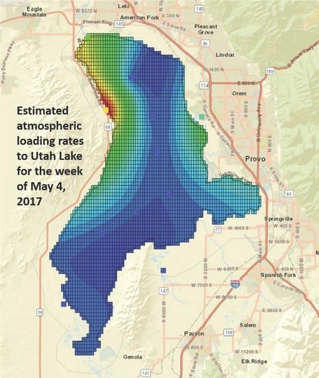
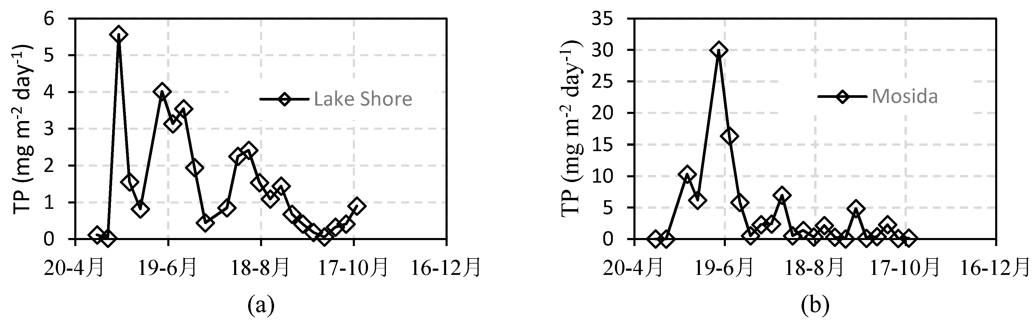
3.2. Phosphorous Load Calculation

Table 3. Summary for total phosphorous (TP) concentration and load data from May 2017 through December 2017.

Site	No. of Data	Mean TP Concentrations (mg/L)		Rain	Total TP Load Rate (mg m−2 day−1)
		Wet	Dry	cm(in)/Week	Mean	S.D.	Skewness
Lake Shore	41	0.68	0.38	0.64(0.25)	1.33	1.95	0.82
Mosida	38	0.22	1.10	0.30(0.12)	2.77	5.63	2.55
Saratoga Springs	44	0.60	5.15	0.43(0.17)	31.38	88.73	2.14
Pump Station	38	0.59	0.85	0.41(0.16)	3.78	20.14	4.68
Orem WWTP 1	27	1.62	0.39	0.28(0.11)	1.26	2.65	3.33
Average	38	0.74	1.57	0.41(0.16)	8.10	23.82	2.70

¹ Waste Water Treatment Plant (WTTP).

presents the TP results as mean TP concentrations at each sample site separated by deposition type, the weekly average precipitation, and the mean TP load rate at each sample site with standard deviation, and skewness values for the loading data. The average loading across all the sites was 8.10 mg of TP m⁻² day⁻¹, with mean values for the individual sites ranging from 1.26 to 31.38 mg of TP m⁻² day⁻¹ at Orem WWTP and Saratoga Springs, respectively. Standard deviation of the loading rates were high, larger than the mean values. The skewness values are all greater than 0, with an average value of 2.7, which indicates that the samples are skewed right. This means that the bulk of the data are in the lower range with a few larger values (i.e., long tail towards the higher values). The coefficient of variation (i.e., mean divided by standard deviation), calculated using all the data, was 0.34.

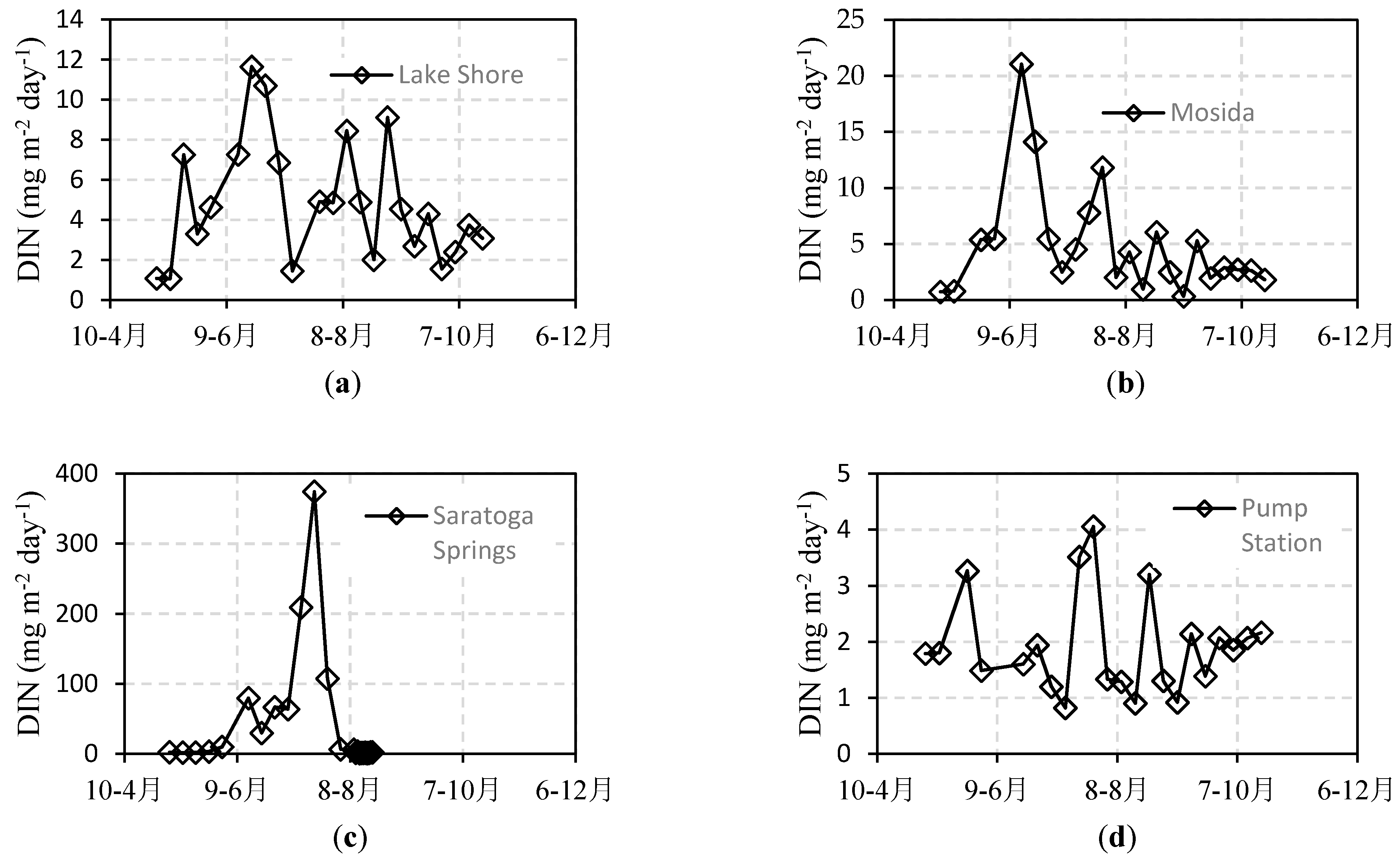
3.3. Nitrogen Load Calculation

Table 4. Summary for dissolved inorganic nitrogen (DIN) deposition data from May 2017 through December 2017.

Site	No. of Data	Mean DIN Concentrations (mg/L)		Rain	Total DIN Load Rate (mg m−2 day−1)
		Wet	Dry	cm(in)/Week	Mean	S.D.	Skewness
Lake Shore	41	4.30	1.15	0.64(0.25)	4.09	4.06	0.47
Mosida	38	2.29	1.50	0.30(0.12)	4.17	4.74	1.21
Saratoga Springs	44	4.86	6.00	0.43(0.17)	36.06	124.62	3.31
Pump Station	38	4.29	0.38	0.41(0.16)	1.59	2.33	2.31
Orem WWTP	27	7.55	1.33	0.28(0.11)	5.23	4.60	3.04
Average	38	4.66	2.07	0.41(0.16)	10.23	28.07	2.07

presents the DIN results as mean DIN concentrations at each sample site separated by deposition type, the weekly average precipitation, and the mean DIN load rate at each sample site with standard deviation, and skewness values for the loading data. The average DIN loading of all sites is 10.23 mg of N m⁻² day⁻¹. The mean values for the individual sites range from 1.59 to 36.06 mg of N m⁻² day⁻¹ at the Pump Station and Saratoga Springs, respectively. As with the TP data, the standard deviations are high and skewness values are positive—indicating that the data have long tails to the right (large outliers). The coefficient of variation, calculated for all the data, was 0.36, very similar to that computed for the TP data.

3.4. Site Comparison

Deposition rates varied both spatially and temporally among sample locations. Figure 4 and Figure 5 show the temporal variation for TP and DIN, respectively for each sample site. Precipitation data showed no significant differences among the sites. Dry deposition rates showed few site-to-site differences aside from the Saratoga Springs site.

Table 3 and Table 4 show that TP and DIN deposition rates at Saratoga Springs were significantly higher than at the other sites. The TP deposition rate differences between Saratoga Springs and the other sites all have p-values < 0.005 (0.5%). Traditionally, p-values < 0.05 (5%) are used to determine if the difference is statistically significant, our p-values are an order of magnitude lower, indicating that it is unlikely that the difference is due to chance. We attribute this difference mainly to local nutrient sources in the area and regional weather patterns. Near the Saratoga Springs sample site there are large areas of bare earth that have high concentrations of TP. This site is also close to areas with both agricultural and excavation activities at a gravel pit. In addition to these issues, storms tend to move across Utah Lake from desert areas with high dust to the northwest and west, crossing this site before reaching the lake. Other sample sites are separated from the western Utah desert areas by agricultural or urban areas that do not generate as much dust. We discuss these issues in detail later in the manuscript.

3.5. Total Deposition

As described in the geostatistical methods section, we used kriging to interpolate deposition rates across Utah Lake to estimate a total deposition loading over the eight month sampling period. We used the same process for both TP and DIN. Because of the large temporal variations in deposition rates, we did not estimate annual deposition, but only estimated total deposition during the sampling period.

We estimated two different total deposition values. For the higher estimate, we included all samples collected during the study. For the lower estimate, we excluded all the samples we deemed contaminated from the analysis. Contamination was defined as the presence of any visible particles in the collection bucket. These two estimates provide bounding values for the actual deposition that occurred during the sampling period. We believe the lower estimate bounds the deposition rates because it excludes all loads from dust particles, insect bodies, and other legitimate sources of nutrients. We believe the upper estimate bounds the deposition rates because it includes some contamination sources that may be local and not significantly extend into the lake itself.

For the higher value (computed using all the samples), we estimated that the total deposition loading of TP and DIN were 350 Mg (tons) and 460 Mg (tons), respectively, over the 8-month period. For the lower value (contaminated samples excluded), the total deposition loading of TP and DIN were 8 Mg (tons) and 46 Mg (tons), respectively, for the 8-month period.

Figure 6, Figure 7, Figure 8 and Figure 9 show the weekly atmospheric deposition rates for TP and DIN over the study period. Figure 6 and Figure 7 present the lower and upper estimate values for TP and DIN, respectively. Because of the scale, it is difficult to see the variation in the lower estimate values. Figure 8 and Figure 9 present the weekly lower estimates for TP and DIN, respectively. These figures show considerable temporal variation in both the high and low estimates, the upper estimate has the highest rates in the June–August period while the lower estimate has higher rates in the November–December period. In the latter period, November–December, the differences between the upper and lower bounds are small as contaminated samples are rare during this time.

Figure 10 shows an example distribution of TP loading for the week ending 11 May 2017. Figure 6 shows that for this week, the difference between the maximum and minimum TP loading estimates was relatively small. In Figure 10, deposition rates range from approximately 100 mg m⁻² day⁻¹ at the Saratoga Springs site (northwest shore) to approximately 0.01 mg m⁻² day⁻¹ near the center and southeast portion of the lake—approximately four orders of magnitude lower. This map shows that our choice of variogram parameters, specifically the smaller range value, used with the kriging algorithm limits the spatial influence of the high samples, with the majority of the lake tending toward background levels (blue in the figure). The green color represents values about two orders of magnitude below the red values.

4. Discussion

4.1. Wet and Dry Deposition Rates

Wet deposition rates are more spatially correlated while dry deposition rates show more local variation. Wet deposition is the result of nutrients dissolved in precipitation; while there is some local influence on this process, most nutrients are dissolved into the rain higher in the atmosphere, away from most local variation. This explains why these data are more similar. Dry deposition rates are heavily influenced by local processes and phenomena, such as dust clouds or other near-ground sources such as insects. In addition, the dry deposition sample buckets had water in the bucket to trap the dry material. Some of the material trapped was larger in size, such as wind-borne vegetative matter or insects. The largest dry deposition rates occurred at Saratoga Springs during the summer months with rates significantly higher than any of the other sites (see Figure 4). We attribute some of these high values to a terrestrial bee, Halictidae Lasioglossum. During the summer period, sample buckets had numerous bee bodies in the water. As noted above, these bodies were removed before sample analysis, but having been present in the water during the week, they significant raise the amount of nutrients in the samples. Also, as noted, the Saratoga Springs site had more local contribution from dust—which is also higher in the dry summer months. This, and other site differences, appeared to be mainly based on site characteristics; high TP deposition rates were found near agricultural and excavation areas. The west side of Utah Lake is impacted by a large gravel pit and agricultural practices, and these dust sources combined with high phosphorous levels in the soil are likely contributing to higher levels of TP. Other studies have reached similar conclusions that local sources can contribute significant nutrient loadings [31].

4.2. Local Sources versus Global Sources

As discussed, most atmospheric transport methods are designed to minimize contributions from local sources and are intended to characterize long-range transport [24]. An important issue in this study is how far onto the lake the influence from local nutrient sources extends and at which point nutrients associated with long-range transport (i.e., regional, global) become the major source. The sample sites we used around Utah Lake record a combination of both local and long-range sources. We designed this study to characterize local source contributions because Utah Lake is surrounded by urban, industrial, and agricultural land uses, and soils in the area have high nutrient content. Standard methods developed to study long-range nutrient transport would view these sample sites as being compromised because they are close to dust sources, agricultural regions, and other activities that can cause nutrients to become airborne [24]. However, since we are developing a nutrient loading based on atmospheric deposition, these local sources are important and represent actual contributions to nutrient loads on the lake; local sources are not viewed as contaminated samples. Our sampling sites were not selected to be free of local sources but rather to be representative of atmospheric deposition on the lake surface.

The high spatial variability in TP loads (see Table 3) suggests that significant portions of the TP deposition load is from local sources and affected by local conditions at the sampling sites. For example, the maximum average TP load was observed at the Saratoga Springs site (31.38 mg of TP m⁻² day⁻¹). We attribute these higher nutrient loadings to the proximity to local dust sources, industrial and agricultural practices, and local soils.

Local sources are highest when dust is suspended during windy storms. In this region, most storms approach from a westerly direction, first arriving on the western shore (represented by the Saratoga Springs site). The Orem WWTP site is on the eastern shore and local dust clouds generated during these storms need to cross the approximately 10-km (6-mile) wide lake before reaching this sample point. The Orem WWTP site has the minimum average TP loading measured during this study of 1.26 mg m⁻² day⁻¹. It is likely that TP deposition rates decrease across the lake in some fashion from the 31.38 to 1.26 mg m⁻² day⁻¹ measured at Saratoga Springs and the Orem WWTP, respectively.

To bound our estimates, as noted above, we assumed that TP deposition rates near the center of the lake were only 0.019 mg m⁻² day⁻¹, which is the value reported in the literature for regional long-range transport [28]. This regional value is two orders of magnitude below the smallest rate we measured of 1.59 mg m⁻² day⁻¹, averaged over the study period, at the Pump Station site. This indicates that our low estimate may be significantly below actual deposition rates. Sampling sites near the lake center will be required to resolve this question.

4.3. Total Deposition

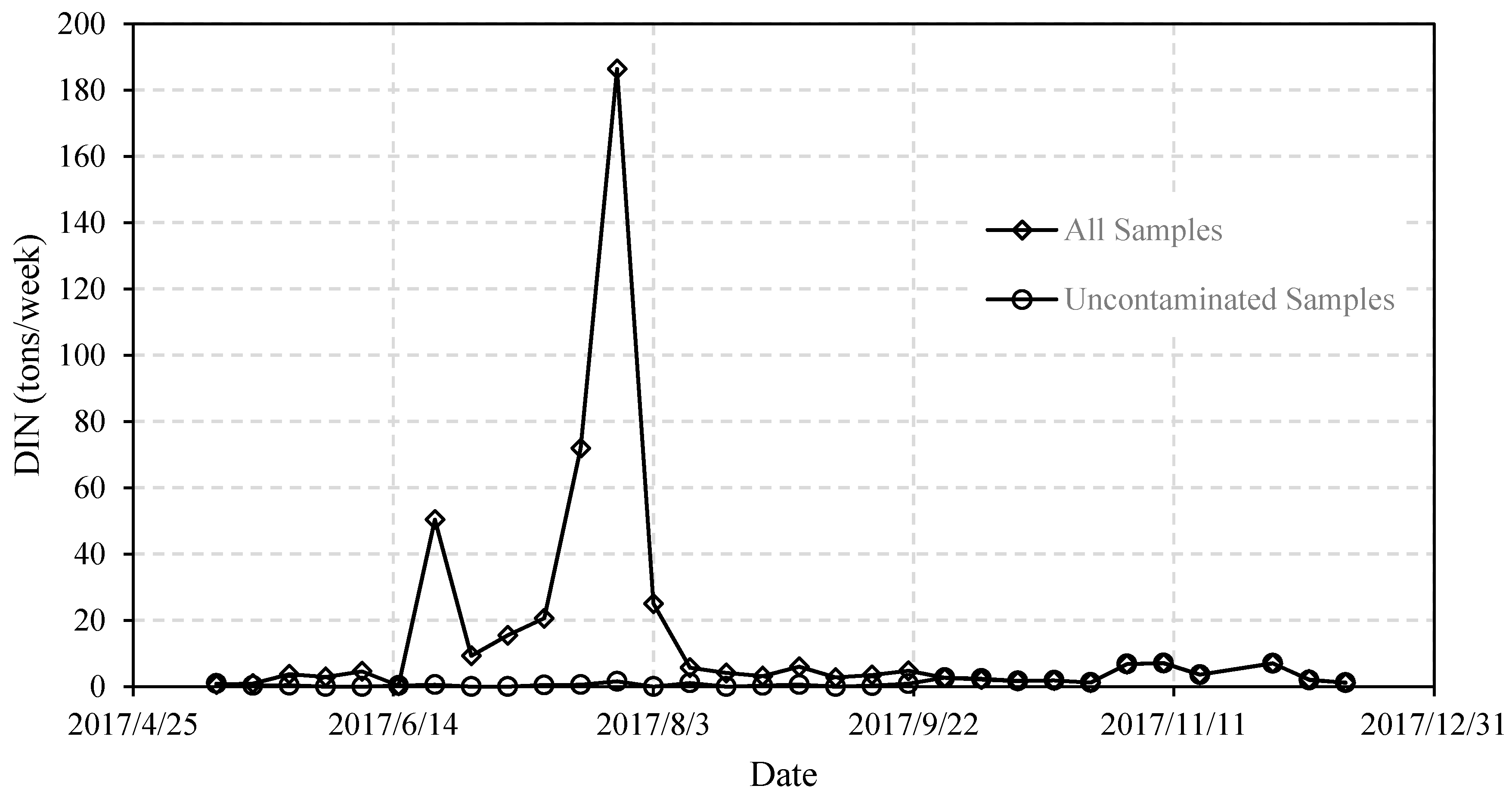
TP and DIN seasonal deposition rates are similar with higher deposition during the late spring and summer months and lower rates during the winter months. Both TP and DIN deposition rates were dominated by dry deposition (i.e., particulate matter rather than dissolved). Maximum deposition occurred in July and early August. This temporal pattern of TP and DIN deposition is shown in Figure 6 and Figure 7, respectively.

These seasonal trends agree with many other studies which found that deposition increased in early summer and decreased over the remainder of the summer [32,33,34]. In a review of studies on TP deposition from long-range transport, deposition rates showed a wide range. with estimated values between 0.007 to 1.7 mg m⁻² day⁻¹ [35]. Our uncontaminated TP samples used for the lower bound estimate, fall within this range of values. The contaminated TP samples used in the upper bound estimate exceeded this range for 7 weeks during the study period, from 22 June 2017 to 8 August 2017. The period with these higher values is shown on Figure 6, but with units of total deposition (Mg (tons) week⁻¹) as the unit rate was converted to lake deposition rates.

Literature-reported nitrogen deposition ranges were smaller than those of TP deposition. We compared our DIN data to the NADP wet deposition data for 2014 in Utah. NADP-reported rates ranged from 2.14 to 8.42 mg m⁻² year⁻¹ [24] while our measured rates ranged from 0.04 to 24.82 mg m⁻² year⁻¹. Our measured values appear to be reasonable when compared to other studies [31,33], again with the higher values used for the upper bound being attributed to local sources.

We did not attempt to determine what percentage of these loads were bio-available. We expect that the majority of the DIN is in bioavailable forms as is the wet TP loadings as the majority of these samples only contained dissolved phosphate. The dry TP loadings contained significant local soils and dust with a portion of the phosphorous in a mineral form. Local sediment and soil samples have phosphorous concentrations in the 600–1900 mg/kg range with 40–60% of this phosphorous in the water soluble, salt extractable, or iron-bound phases, all of which can easily release bioavailable phosphorous to the water column [15,36,37].

4.4. Contamination

Contamination is a problem in deposition studies, mainly due to a lack of agreement as to how to delineate the boundaries for the area being studied as this defines what is regarded as contamination. For example, long-range transport studies view local sources as contamination that do not contribute to additional loading because the nutrients are from the same areas—that is, no new nutrients are introduced or transported into the region. For these studies, local sources are contamination because they represent internal recycling within the local system, not new nutrients [23]. For long-range transport studies, these local contamination sources include excavation and agriculture and also includes nutrients from birds and insects.

For this study, we are attempting to bound nutrient loads to the water column in a lake or reservoir. For this purpose, the study should include all of the sources that provide nutrients to the lake, especially during the main algal-growth season. This definition includes shoreline or other local sources as nutrients from these sources provide additional loads to the lake. These differences in the goals and scope of the studies make the selection of sample sites different. For long-range studies, sites should be isolated, away from local dust sources or activities that could contribute local nutrients to the sample bucket as outlines by the NADP [24]. For studies trying to characterize nutrient loads to lakes or reservoirs, local sources, such as dust from shoreline soils and activities such as agriculture or excavations, can contribute significant loads to the water column. For this study, we viewed all these local sources as legitimate nutrient sources which increase the total load to the water column.

In this study, 43% of the collected samples were contaminated to some degree. Insects were the main source of contamination, with the terrestrial bee Halictidae Lasioglossum as the most common insect.

4.5. Upper and Lower Bound Estimates

Our upper estimate was computing using both contaminated and uncontaminated samples. Our lower estimate did not use contaminated samples. The contaminated samples mostly contained contributions from birds and insects with little plant materials. We manually removed all large particulates (such as insect bodies) from the samples before analysis.

Our lower estimate was computed using only the uncontaminated samples. These samples still represent both long-range and short-range transport because of the location of the sampling sites near the lake shore. That is, we expect them to be influenced by local dust sources (e.g., high nutrient soils), agricultural or other anthropogenic sources. We do not expect this loading to only be deposited near the shore, but to be carried significant distances into the lake. To provide a conservative lower estimate, we assumed that deposition rates approached long-range deposition values at the middle of the lake. We feel this is a conservative lower bound because wind transport is mainly west-to-east, samples on the eastern shore had deposition rates more than two orders of magnitude higher than the background, long-range deposition values we used as characteristic for the center of the lake. Actually, deposition values are probably closer to those measured on the eastern shore, though we have no data to support this assertion.

4.6. Future Work

More work is required to characterize deposition rates within Utah Lake. We expect them to be higher than our lower bound estimate as we believe that local sources influence deposition across the entire lake, not just the near shore area. We also expect deposition rates to vary, not only within a year, but over longer periods. For example, dry hot years would likely have higher dust source contributions than wet years, though the wind associated with storms during wet years may also cause higher rates. A long-term study is required to better understand actual deposition. We do think that our upper and lower estimates with their associated large range, effectively bound the actual rates.

5. Conclusions

Many studies have indicated that atmospheric deposition can be an important component of the nutrient budget of a lake. We collected nutrient data weekly at five locations, situated around Utah Lake. The sample locations were selected to characterize atmospheric deposition. The sites are approximately equally spaced around the lake with locations chosen to match the main local land use. We collected both wet and dry nutrient deposition using methods and samplers following recommendations from the National Atmospheric Deposition Program (NADP) [24]. Almost half of our samples, 43%, showed contamination based on NADP guidelines. However, for this study, we viewed this contamination as legitimate nutrient sources to the water column—not as local nutrient recycling as does the NADP. Rather than trying to provide a best estimate for nutrient deposition to Utah Lake, we estimated a lower and upper bound. The lower bound was estimated using only uncontaminated samples and the upper bound was estimated using all the samples. To address depletion as local sources moved across the lake, we assumed that the center of the lake only experienced deposition from the long-range background—a rate more than two orders of magnitude below our lowest rates measured on the eastern shore and nearly four orders of magnitude from the highest rates measured on the western shore. We did not estimate annual rates, as we only had 8 months of data and the data showed significant temporal variation.

Our estimates of the 8-month nutrient load indicate that the atmosphere contributes between 8 to 350 Mg (tons) of TP and 46 to 460 Mg (tons) of DIN during this period. Dry TP deposition represents the bulk of seasonal deposition and the most important fraction of total deposition. The largest atmospheric nutrient deposition loading occurs during the summer months which is the most critical time for phytoplankton growth. Since the summer is when the algal growth is the greatest, it is important to note that the impact of atmospheric deposition to Utah Lake it even greater than if it were spread evenly during the year.

Studies of Utah Lake have concluded that about 17 Mg (tons) of phosphorus per year and 200 Mg (tons) of nitrogen per year would be sufficient to support the algal growth currently occurring in the lake, which is deemed to be negatively impacted from high nutrient loads [9]. Even our low estimates of 8 and 46 Mg (tons) for only 8 months are approximately ½ and ¼ of the TP and DIN loads, respectively estimated to support eutrophic conditions. We assert that these lower bound estimates are significantly below the actual values because of our conservative use of the long-range transport values for the center of the lake. Our high bound estimates of 350 and 460 Mg (tons) of TP and DIN, respectively, are well above the loads estimated to support eutrophic conditions. We feel that this higher estimate is an upper bound, but that these values are not unrealistic.

This study shows that atmospheric nutrient deposition contributes sufficient loadings to support eutrophic lake conditions. While this study was specific to Utah Lake, these results should guide water managers at other locations. Most lake total maximum daily load (TMDL) studies do not include atmospheric deposition. This could be a major oversight and may indicate why some water bodies do not respond as well as expected to nutrient reductions in inflows though we have no data on other locations.

References

1. Anderson, D.M.; Glibert, P.M.; Burkholder, J.M. Harmful algal blooms and eutrophication: Nutrient sources, composition, and consequences. Estuaries 2002, 25, 704–726. [Google Scholar] [CrossRef]
2. Heisler, J.; Glibert, P.M.; Burkholder, J.M.; Anderson, D.M.; Cochlan, W.; Dennison, W.C.; Dortch, Q.; Gobler, C.J.; Heil, C.A.; Humphries, E. Eutrophication and harmful algal blooms: A scientific consensus. Harmful Algae 2008, 8, 3–13. [Google Scholar] [CrossRef] [PubMed] [Green Version]
3. Cole, J.J.; Caraco, N.F.; Likens, G.E. Short-range atmospheric transport: A significant source of phosphorus to an oligotrophic lake. Limnol. Oceanogr. 1990, 35, 1230–1237. [Google Scholar] [CrossRef]
4. Jassby, A.D.; Reuter, J.E.; Axler, R.P.; Goldman, C.R.; Hackley, S.H. Atmospheric deposition of nitrogen and phosphorus in the annual nutrient load of lake tahoe (california-nevada). Water Resour. Res. 1994, 30, 2207–2216. [Google Scholar] [CrossRef]
5. Lewis, W.M. Precipitation chemistry and nutrient loading by precipitation in a tropical watershed. Water Resour. Res. 1981, 17, 169–181. [Google Scholar] [CrossRef]
6. Schindler, D.; Newbury, R.; Beaty, K.; Campbell, P. Natural water and chemical budgets for a small precambrian lake basin in central canada. J. Fish. Board Can. 1976, 33, 2526–2543. [Google Scholar] [CrossRef]
7. PSOMAS. Utah Lake Tmdl: Pollutant Loading Assessment & Designated Beneficial Use Impairment Assessment; PSOMAS: Salt Lake City, UT, USA, 2007. [Google Scholar]
8. DWQ. Utah Lake Water Quality Work Plan 2015–2019; Utah State Division of Water Quality: Salt Lake City, UT, USA, 2016. [Google Scholar]
9. Merritt, L.B.; Miller, A.W. Interim Report on Nutrient Loadings to Utah Lake; Report to the Utah Department of Water Quality: Salt Lake City, UT, USA, 2016. [Google Scholar]
10. Sorokin, C.; Krauss, R.W. The effects of light intensity on the growth rates of green algae. Plant Physiol. 1958, 33, 109. [Google Scholar] [CrossRef] [PubMed]
11. Brown, T.E.; Richardson, F.L. The effect of growth environment on the physiology of algae: Light intensity. J. Phycol. 1968, 4, 38–54. [Google Scholar] [CrossRef] [PubMed]
12. Lee, G.F.; Rast, W.; Jones, R.A. Water report: Eutrophication of water bodies: Insights for an age old problem. Environ. Sci. Technol. 1978, 12, 900–908. [Google Scholar] [CrossRef]
13. Hansen, C.; Swain, N.; Munson, K.; Adjei, Z.; Williams, G.P.; Miller, W. Development of sub-seasonal remote sensing chlorophyll-a detection models. Am. J. Plant Sci. 2013, 4, 21. [Google Scholar] [CrossRef]
14. Hansen, C.H.; Dennison, P.; Burian, S.; Barber, M.; Williams, G. Hindcasting water quality in an optically complex system. WIT Trans. Ecol. Environ. 2016, 209, 35–44. [Google Scholar]
15. Abu-Hmeidan, H.Y.; Williams, G.P.; Miller, A.W. Characterizing total phosphorus in current and geologic utah lake sediments: Implications for water quality management issues. Hydrology 2018, 5, 8. [Google Scholar] [CrossRef]
16. Hansen, C.H.; Burian, S.J.; Dennison, P.E.; Williams, G.P. Spatiotemporal variability of lake water quality in the context of remote sensing models. Remote Sens. 2017, 9, 409. [Google Scholar] [CrossRef]
17. Hansen, C.H.; Williams, G.P.; Adjei, Z.; Barlow, A.; Nelson, E.J.; Miller, A.W. Reservoir water quality monitoring using remote sensing with seasonal models: Case study of five central-utah reservoirs. Lake Reserv. Manag. 2015, 31, 225–240. [Google Scholar] [CrossRef]
18. Carlson, R.E. A trophic state index for lakes. Limnol. Oceanogr. 1977, 22, 361–369. [Google Scholar] [CrossRef] [Green Version]
19. Larsen, D.; Mercier, H. Lake phosphorus loading graphs: An alternative. In National Technical Information Service; NTIS: Springfield, VA, USA, 1975; Volume PB-243 869, p. 4. [Google Scholar]
20. Nanus, L.; Campbell, D.H.; Ingersoll, G.P.; Clow, D.W.; Alisa Mast, M. Atmospheric deposition maps for the rocky mountains. Atmos. Environ. 2003, 37, 4881–4892. [Google Scholar] [CrossRef]
21. Uttormark, P.D.; Chapin, J.D.; Green, K.M. Estimating Nutrient Loadings of Lakes from Non-Point Sources; Office of Research and Development, U.S. Environmental Protection Agency: Washington, DC, USA, 1974.
22. Welch, H.E.; Legault, J.A. Precipitation chemistry and chemical limnology of fertilized and natural lakes at saqvaqjuac, nwt. Can. J. Fish. Aquat. Sci. 1986, 43, 1104–1134. [Google Scholar] [CrossRef]
23. Ahn, H.; James, R.T. Variability, uncertainty, and sensitivity of phosphorus deposition load estimates in south florida. Water Air Soil Pollut. 2001, 126, 37–51. [Google Scholar] [CrossRef]
24. NADP. Nadp Site Selection and Installation; National Atmospheric Deposition Program: Madison, WI, USA, 2014. [Google Scholar]
25. Utah Agrc: Automated Geographic Reference Center. Available online: https://gis.utah.gov/data/ (accessed on 10 July 2017).
26. NOAA. Climatological Data Publications. Available online: https://www.ncdc.noaa.gov/IPS/cd/cd.html (accessed on 5 March 2018).
27. Anderson, K.A.; Downing, J.A. Dry and wet atmospheric deposition of nitrogen, phosphorus and silicon in an agricultural region. Water Air Soil Pollut. 2006, 176, 351–374. [Google Scholar] [CrossRef]
28. Mahowald, N.; Jickells, T.D.; Baker, A.R.; Artaxo, P.; Benitez-Nelson, C.R.; Bergametti, G.; Bond, T.C.; Chen, Y.; Cohen, D.D.; Herut, B. Global distribution of atmospheric phosphorus sources, concentrations and deposition rates, and anthropogenic impacts. Glob. Biogeochem. Cycles 2008, 22. [Google Scholar] [CrossRef] [Green Version]
29. Gomolka, R.E. An Investigation of Atmospheric Phosphorus as a Source of Lake Nutrient; University of Toronto: Toronto, ON, Canada, 1975. [Google Scholar]
30. AQUAVEO. Ground Water Modeling System 10.2.4. Available online: https://www.aquaveo.com/software/gms-groundwater-modeling-system-introduction (accessed on 5 March 2018).
31. Hendry, C.; Brezonik, P.; Edgerton, E. Atmospheric Deposition of Nitrogen and Phosphorus in Florida [Contaminants, Nutrients in Rainfall]; Food and Agriculture Organization: Rome, Italy, 1981. [Google Scholar]
32. Linsey, G.; Schindler, D.; Stainton, M. Atmospheric deposition of nutrients and major ions at the experimental lakes area in northwestern ontario, 1970 to 1982. Can. J. Fish. Aquat. Sci. 1987, 44, s206–s214. [Google Scholar] [CrossRef]
33. Shaw, R.; Trimbee, A.; Minty, A.; Fricker, H.; Prepas, E. Atmospheric deposition of phosphorus and nitrogen in central alberta with emphasis on narrow lake. Water Air Soil Pollut. 1989, 43, 119–134. [Google Scholar] [CrossRef]
34. Delumyea, R.; Petel, R. Wet and dry deposition of phosphorus into lake huron. Water Air Soil Pollut. 1978, 10, 187–198. [Google Scholar] [CrossRef]
35. Newman, E. Phosphorus inputs to terrestrial ecosystems. J. Ecol. 1995, 713–726. [Google Scholar] [CrossRef]
36. Carling, G.T.; Randall, M.; Nelson, S.; Rey, K.; Hansen, N.; Bickmore, B.; Miller, T. Characterizing the Fate and Mobility of Phosphorus in Utah Lake Sediments. In Proceedings of the AGU Fall Meeting Abstracts, New Orleans, LA, USA, 11–15 December 2017. [Google Scholar]
37. Merrell, P.D. Utah Lake Sediment Phosphorus Analysis; Brigham Young University: Provo, UT, USA, 2015. [Google Scholar]
Figure 1. Utah Lake is a large freshwater lake in northern Utah which has a surface area of about 360 square km (140 square miles) with an average depth of 2.7 m (9 feet) and a maximum depth of only 4.3 m (14 feet). Also shown on the map are the five atmospheric deposition sampling sites used in this study.
Hydrology 05 00045 g001
Figure 2. The Jordan River basin that contains both the inflows and outflow for Utah Lake (figure created from [25]).
Hydrology 05 00045 g002
Figure 3. Utah Lake coverage showing the eleven points used in interpolation.
Hydrology 05 00045 g003
Figure 4. Temporal variations in TP by sample locations: (a) Lake Shore; (b) Mosida; (c) Saratoga Springs; (d) Pump Station; (e) Orem WWTP.
Hydrology 05 00045 g004aHydrology 05 00045 g004b
Figure 5. Temporal variations in DIN by sample locations: (a) Lake Shore; (b) Mosida; (c) Saratoga Springs; (d) Pump Station; (e) Orem WWTP.
Hydrology 05 00045 g005aHydrology 05 00045 g005b
Figure 6. Utah Lake TP seasonal loading weekly estimates, both high (all samples) and low (uncontaminated samples) estimates.
Hydrology 05 00045 g006
Figure 7. Utah Lake DIN seasonal loading weekly estimates, both high (all samples) and low (uncontaminated samples) estimates.
Hydrology 05 00045 g007
Figure 8. TP lower estimates of weekly loadings (uncontaminated samples).
Hydrology 05 00045 g008
Figure 9. DIN lower estimates of weekly loadings (uncontaminated samples).
Hydrology 05 00045 g009
Figure 10. Example map showing the spatial deposition rates for TP for the period of 4 May 2017 through 11 May 2017. The map shows that the pseudo sample sites in the center of the lake, which represent regional background rates, strongly influence the distribution. The colors are on a logarithmic scale with red approximately 100 mg m−2 day−1 and blue about 0.01 mg m−2 day−1 spanning four orders of magnitude. This map shows that the influence of high values at shoreline stations do not reach significantly into the lake because of the small variogram range used for kriging.
Hydrology 05 00045 g010