Article

Revisiting Cent-Fonts Fluviokarst Hydrological Properties with Conservative Temperature Approximation

by
Philippe Machetel
1,* and
David A. Yuen
2,3
1
Laboratoire Géosciences Montpellier, CNRS/UM2, 34095 Montpellier CEDEX 9, France
2
Minnesota Supercomputing Institute and Department of Earth Sciences, University of Minnesota, 310 Pillsbury Dr. SE, Minneapolis, MN 55455, USA
3
School of Environmental Studies, China University of Geosciences, 388 Lumo Road, Wuhan 430074, China
*
Author to whom correspondence should be addressed.
Hydrology 2017, 4(1), 6; https://doi.org/10.3390/hydrology4010006
Submission received: 28 November 2016 / Revised: 6 January 2017 / Accepted: 16 January 2017 / Published: 24 January 2017
(This article belongs to the Special Issue Groundwater Flow)

Abstract

:
We assess the errors produced by considering temperature as a conservative tracer in fluviokarst studies. Heat transfer that occurs between karstic Conduit System (CS) and Porous Fractured Matrix (PFM) is the reason why one should be careful in making this assumption without caution. We consider the karstic aquifer as an Open Thermodynamic System (OTS), which boundaries are permeable to thermal energy and water. The first principle of thermodynamics allows considering the enthalpy balance between the input and output flows. Combined with a continuity equation this leads to a two-equation system involving flows and temperatures. Steady conditions are approached during the recession period or during particular phases of pumping test experiments. After a theoretical study of the error induced by the conservative assumption in karst, we have applied the method to revisit the data collected during a complete campaign of pumping test. The method, restricted to selected data allowed retrieving values of base flow, mixing of flow, intrusions of streams, and aquifer answer to drawdown. The applicability of the method has been assessed in terms of propagation of the temporal fluctuations trough the solving but also in terms of conservative assumption itself. Our results allow retrieving the main hydrological properties of the karst as observed on field (timed volumetric samplings, geochemical analyses, step pumping test and allogenic intrusion of streams). This consistency argues in favor of the applicability of the conservative temperature method to investigating fluviokarst systems under controlled conditions.

1. Introduction and Presentation of Cent-Fonts Fluviokarst

This paper addresses the issue of using the water temperature as a conservative tracer for karstic functioning studies. Whereas costly investments are often necessary to evaluate the potential of karstic aquifers, temperature records may bring cheap method for obtaining complementary information. However underground flows undergo heat transfers with the embedding rocks by advection and by conduction. Despite of this difficulty several studies used temperature as a mixing tracer. Several works [1,2] study the water exchanges between underground flows and surface stream. Others [3] retrieved aquifer recharges solving heat transport equation constrained by measurements of vertical temperature. Slow and rapid equilibrations between ground water and aquifer rocks have been analyzed [4] to study the dynamics of exchanges in fractured carbonate systems. Genthon et al. [5] determined the deep preferential path of rainfall water in caves from annual temperature variations of spring. This author also used temperature to determine limestone drainage in lagoon by removing the tidal component and emphasizing its poor correlation with rain temperature [6]. This short list is far to be exhaustive.
As mentioned in the following theoretical part of this work, the formal applicability of the conservative temperature approximation depends on the existence steady conditions that are never perfectly verified in nature. The question consists of estimating the outcome of this assumption. Indeed, our work is not the first to address this problem. In spite of disturbances due to meteorological conditions, Karanjac and Altug [7] used temperature records to characterize the recharge area, transmissivity and hydraulic regime of karst. Following Stonestrom and Constantz [8], O’Driscoll and DeWalle [9] studied the stream-ground water temperature interactions from stream-air temperature fluctuations. They used weekly averaging and equilibrium temperature concepts [10,11,12]. All these studies rely on damping of diurnal or seasonal variations of temperature records. This is done either by time averaging [13] or by natural damping of temperature fluctuations by depth [14,15]. It is clear that the method presented in this work is not adapted to transient flow or rapidly varying water conditions. Conversely, many situations as recession in karst undergo naturally damping of the temporal fluctuations both for temperatures and flows.
These preliminary considerations justify the interest to study the karst systems as an Open Thermodynamic Systems (OTS), that is to say a “black box” that exchanges water and heat energy with its surrounding environment. However, let us try to describe the thread of this paper. The following part of the present Section 1 recalls the hydrological description of the Cent-Fonts site and its consistency with the White’s fluviokarst model. Thus, we benefit of an exceptional set of high quality data recorded during the 2005 Cent-Font pumping tests and preliminary studies. This will provide a fair opportunity to test the method. Section 2 displays theory and resulting equations on a reduced form of the White’s model considered as an OTS. Section 3 describes the available data that will be revisited and Section 4 illustrates the application of the method to these selected data. The results are discussed in the “Summary and discussion” Section 5.
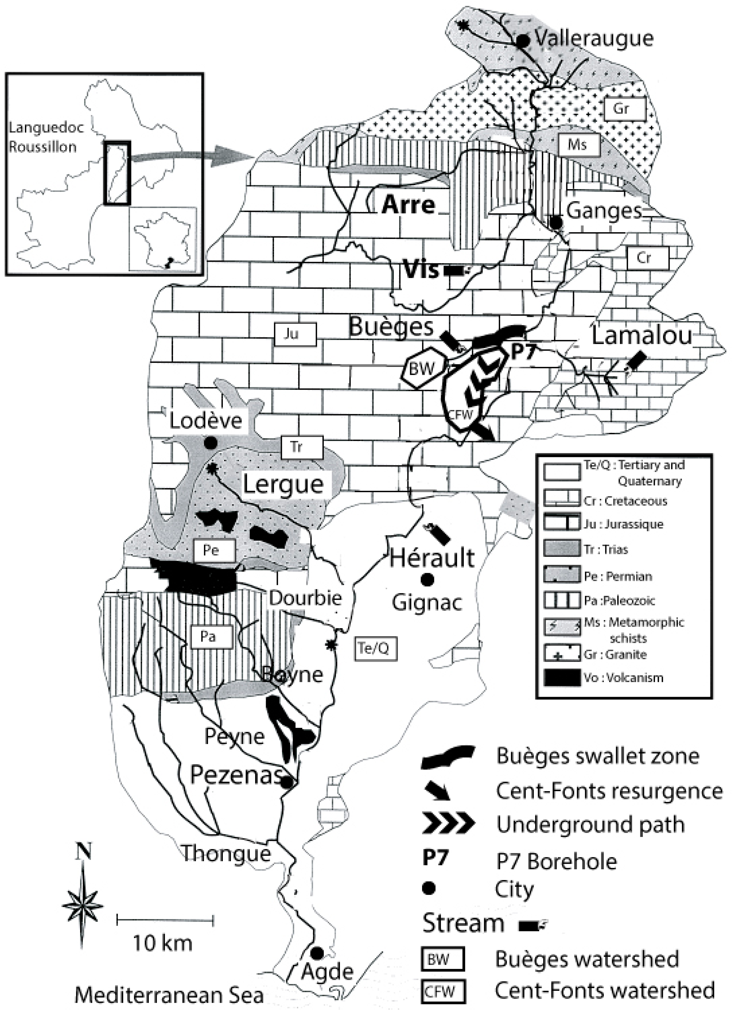
The Cents-Fonts resurgence is the only free-flowing of an underground drainage basin that covers 40 km2 in the median part of Hérault River (Figure 1). The surface of the watershed reaches 60 km2 considering the Buèges stream. It stretches in outcrops of thick calcareous and dolomite massifs (Middle and Upper Jurassic). Since several decades, many geological, geochemical and hydrological studies focused on the potential spring water production of this site (i.e., [16,17,18,19,20,21,22,23,24,25,26,27]).
The Buèges stream and the Cévennes fault mark the boundaries of the watershed to the north and northwest, while the altitude of the Hérault River matches the karstic base level to the southeast (Figure 1). Morphologically, the area is a plateau, uplifted of 200 to 500 m during the late Quaternary and eroded during Oligocene. The watershed drains rainfalls through an epikarstic transition zone that supplies the Cent-Fonts resurgence base flow [22]. To the north, Buèges stream flows permanently on Triassic low permeability outcrops however it disappears à few kilometers after Saint-Jean de Buèges where the course crosses a Bathonian, calcareous dolomite swallow zone. After this area, the Buèges stream course follows a valley that remains dry most of the year except after major rainfalls. Then a surface course catches up with Hérault River at a confluence point north of Lamalou stream (Figure 1). Tracing experiments have confirmed the underground path of Buèges stream intrusion from swallow zone to the Cent-Fonts resurgence [17,20].
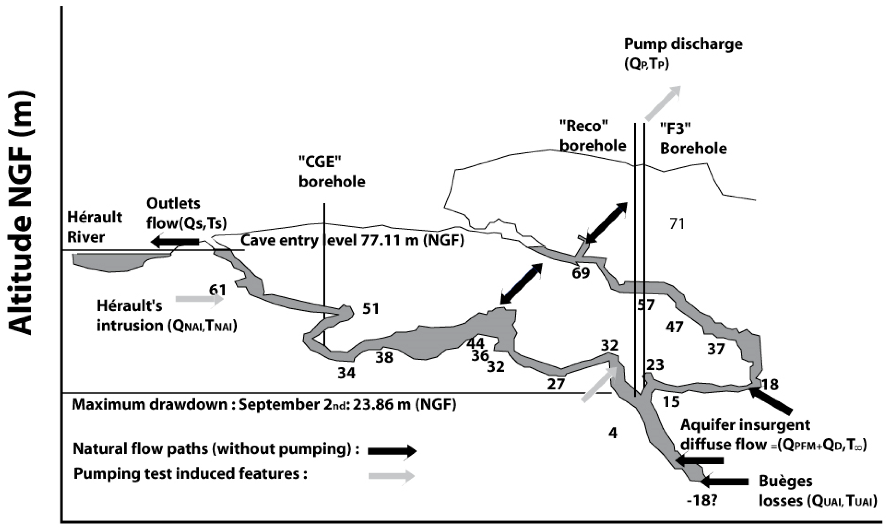
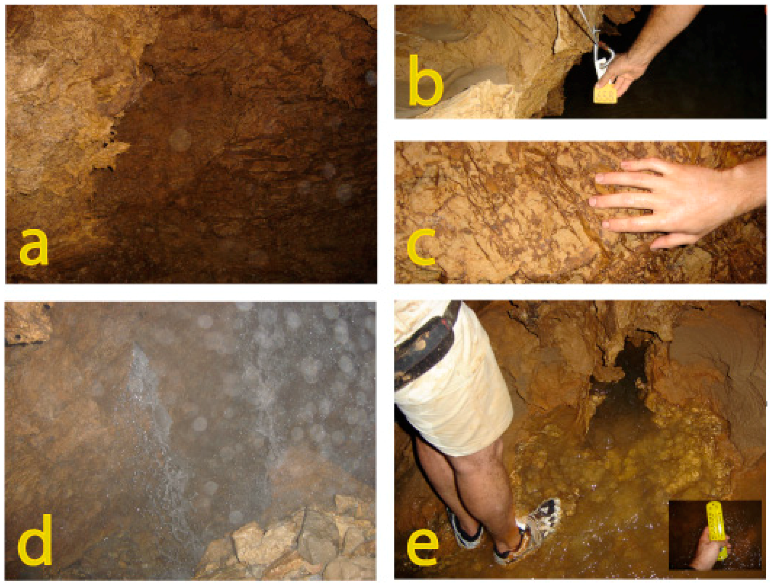
Bathonian, dolomitic layers of Middle Jurassic between 150 and 300 m thick embed the saturated zone of the Cent Fonts fluviokarst near the resurgence. The aquifer also possibly meets an underlying Aalenian-Bajocien layer. The near spring, Conduit System (CS) of the resurgence (Figure 2) has been explored thank to speleological diving that reached 107 m below the base level (Hérault River) [28]. The terminal part of the CS displays an outlet cave, roughly “Y” shaped, with two sub-horizontal branches joining above a deep sub-vertical chimney. The two ends of the “Y” branches open outside. These caves are seldom active except during peak flows. Most of the time, the Cent-Fonts resurgence flows into Hérault River through a shallow network of springs that gush out a few tens of centimeters above the base level. A spring also arises directly through the bottom of the Hérault River bed [20].
The Cent-Fonts karst matches precisely the fluviokarst idea depicted by Smart [29]. Following his definition, fluviokarst consist: in “karst landscapes where the dominant landforms are valleys cut by surface rivers. Such original surface flow may relate either to low initial permeability before caves (and hence underground drains) had developed, or to reduced permeability due to ground freezing in a periglacial environment. In both cases the valleys become dry as karstification improves underground drainage” [30]. White [31,
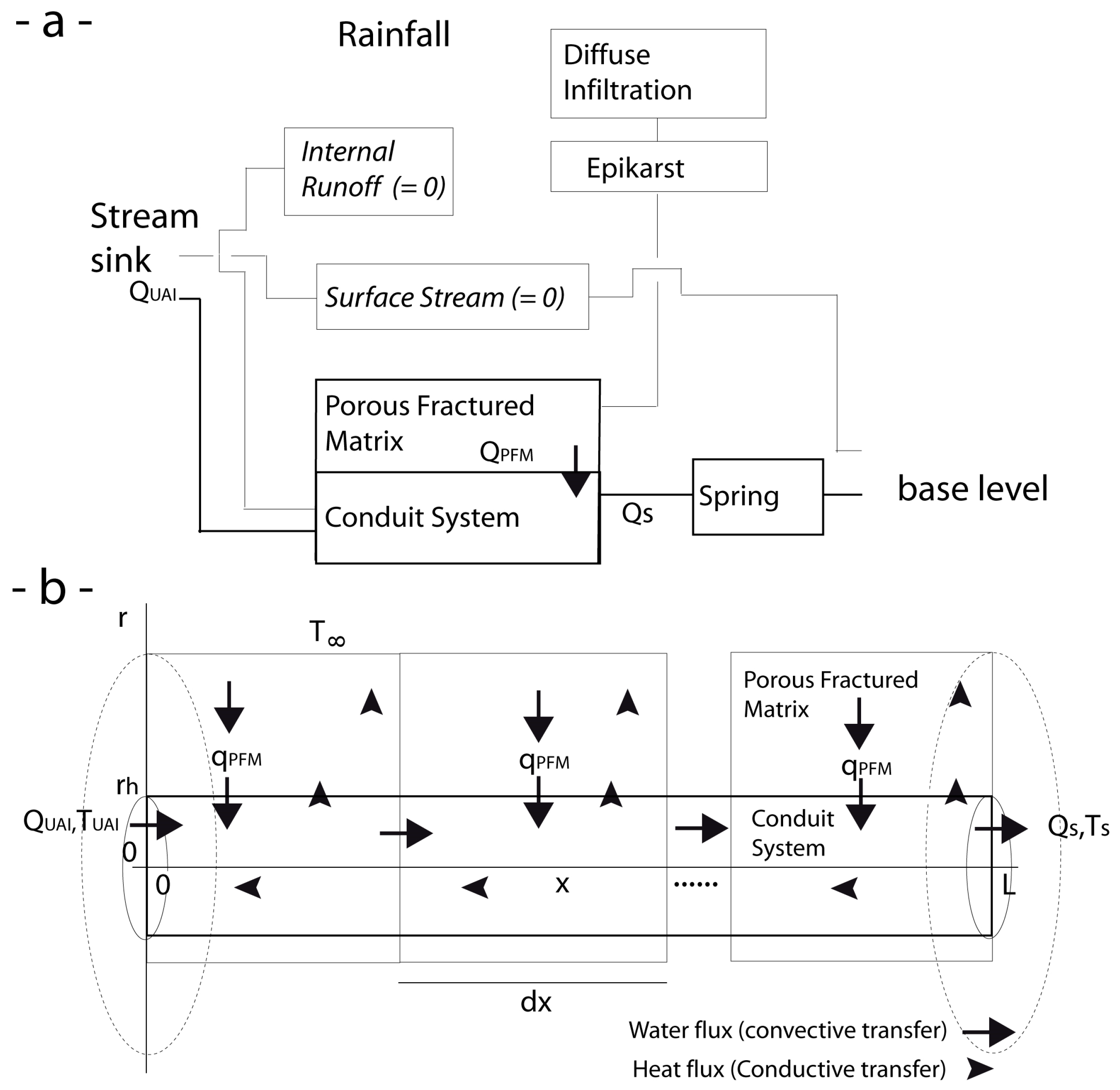
32] proposed a model where the hydrological behaviors are forced by the external boundary conditions. The various recharges in the CS are Allogenic Intrusions, internal Run-off and Porous Fractured Matrix flows. Intrusions of neighbor streams cause the first category of flows. The second results from sporadically floods that occur after heavy rainfalls. The third category gathers percolation flows through soils and epikarstic layer that reach the CS as a Diffuse Infiltration through the fractured and porous rocks of the aquitard (Figure 3a). In the local context of the Cent-Font watershed, the permanent course of Buèges stream matches the Upper Allogenic Stream. Later, at the swallow zone, the Buèges splits into a Surface Stream and an Upper Allogenic Intrusion. The Surface stream forms a non-perennial flow that joins the Hérault River north of Lamalou confluence. The Upper Allogenic Intrusion, QUAI, joins the CS after an underground journey. Table 1 recalls the notations and acronyms of this article. This model also considers the Diffuse Infiltration that percolates through the CS wall. The only output flow of the fluviokarst is the spring, QS, that falls into the Hérault River at the karstic base level.
As mentioned above, the Cent-Fonts resurgence has received much attention since decades (see Ladouche et al. [23] for a review). In September 1992, Cge and the city of Montpellier organized a series of pumping tests but heavy rainfalls and resulting runoff force to stop the experiments after only 16 days. This short time prevents reaching significant aquifer drawdowns despite the high rate of pumping (0.5 m3/s). Thus, this experimentation failed to assess the hydrological properties of the karst and let believe in a high water production potential [33].
Many field observations, such as gauging data of the spring, of the Hérault River and of the Buèges stream have been recorded for several years before the summer 2005 pumping test experiments. New boreholes were drilled. New records of temperatures and discharges were collected in Buèges and Hérault. Temperatures and hydraulic heads were also recorded in the “P7” (Figure 1), “Reco”, “Cge” and “F3” boreholes (Figure 2). The 2005 pumping test campaign started with a sequence of step-drawdown tests. Heavy pumping sequences followed with a high constant rate pumping and a drawdown constant pumping (see Table 1 for accurate chronology). The drawdown induced during these heavy pumping allowed speleological explorations of the Cent-Fonts chimney. It also opened the possibility of in situ timed volumetric gauging and geochemical sampling of Hérault River intrusions in the CS. This rich set of data has been extensively analyzed already [26,34]. The present work aims to revisit part of these data to assess the accuracy of conservative tracer assumption for water temperature. In the following, we will consider that two error sources mainly affect the applicability of the method: (1) The natural temporal instabilities that affect the data series; (2) the effect of conservative temperature assumption itself according to our previous work [35,36].
The next section of the paper recalls the theoretical context of Open Thermodynamic System for fluviokarst. Section 3 describes the data chosen from the 2005 pumping test campaign, Section 4 presents their analysis and accuracy assessments. The results are summarized and discussed in Section 5.

2. Theoretical Context

An Open Thermodynamic System (OTS) does not require a precise knowledge of the locations and shapes of its boundaries to study the balance of the fluxes that enter or quit its Control Volume (CV). In that sense, CS of fluviokarsts are similar to CV of OTS (Figure 3b). We will benefit of this analogy to study the balance of fluxes and energy in the Cent-Fonts fluviokarst CV despite the inaccurate knowledge of its boundaries [35].
In our previous work [36] we assessed the error resulting, in OTS, of conservative temperature assumption within the theoretical context of White’s fluviokarst model. This analysis relied on two successive numerical solving of thermal behavior. The first considered the temperature as a conservative tracer, while the second, following works by Covington et al. [37,38] solved the complete set of energy equations including convective, diffusive and dispersive terms. The amplitude of differences between both results shows the first order of the error due to the conservative assumption. We drew abacus curves of this error versus thermal diffusivity ratio and the Peclet numbers, Prandtl numbers and Reynolds numbers of the CS. The error remains less than 1 percent in the dimensionless space and converges to zero for the most extremes values of karst features. This dimensionless error needs to be rescaled for each singular fluviokarst to calculate its physical amplitude.
In our study, we consider water as a Boussinesq fluid with constant thermal capacity, thermal expansion and density. As a result, water motion forms a zero divergence velocity field in the PFM and in the CS (Equation (1)).
d i v ( v ) = 0
It is possible to convert the volume integrals over fluviokarst CS in flux integrals over the PFM boundaries and hydraulic sections of conduits entering or leaving the CS. Then, the terms of Equation (2) are equal to the input flows into the CS (positive algebraic values, qi) and to the flows escaping from the CS (negative algebraic values, qo). Therefore, the continuity equation leads to the mass conservation equation that links the various flows.
i n p u t q i + o u t p u t q o = 0
The first law of thermodynamics stipulates that the internal energy change of the CV (Equation (3)) corresponds to the balance of the energy differences between all the incoming and outgoing flows (index j) and considering the work done. Thus, the internal energy change (δE) is equal to the summation of: the enthalpy by unit of mass (hj), the potential energy (epot j), the kinetic energy (ecin j), the external heat transfer (δΦj) and the work exchanges (δWj) with the surrounding [39,40].
δ E = j ( h j + e p o t , j + e c i n , j ) d m j + j δ Φ j + j δ W j
In the following, we will consider no chemical contribution to enthalpy and flow transfers with negligible exchange between heat and work. We also will consider steady flux conditions in the CV (we discuss this point later). These hypotheses cancel the internal energy change but also the potential energy and kinetic energy changes. Then, Equation (3) becomes a balance between the specific enthalpies by unit of time of the flows entering (hi) and escaping (ho) the CS (Equation (4)).
i h i ρ i q i + o h o ρ o q o = 0
Now, specific enthalpy depends only on thermal capacity (Cp) and temperature (referred to an arbitrary value Ta) (Equation (5)).
h j = C p j ( T j T a )
Combination of Equations (4) and (5) leads to the enthalpy balance (Equation (6)).
C p i ( T T a ) ρ i q i + C p o ( T o T a ) ρ o q o = 0
Finally, with constant density and thermal capacity Equation (6) reduces to a classical mixing equation (Equation (7)) that links temperatures (°K or °C) and mass transfers in the CS.
i n p u t q i T i + o u t p u t q o T o = 0
Equations (2) and (7) form the basis of a linear system able to discover two unknown flows in the CS (so-called Qk and Ql in Equation (8)).
q k T k + q l T l = o k o l q o T o i k i l q i T i q k + q l = o k o l q o i k i l q i
Thus, these the two unknown flows are (Equation (9)).
q k = 1 ( T k T l ) | o k o l q o T o i k i l q i T i T l o k o l q o i k i l q i 1 | = o k o l q o ( T o T l ) i k i l q i ( T i T l ) ( T k T l ) , q l = o k o l q o i k i l q i q k .
As mentioned above, we will use the theoretical results of Machetel and Yuen [36] to quantify the sensitivity of the model to the conservative enthalpy assumption. However since we assumed that no other sources of heat are present (neither chemical heat, nor work conversion to heat), enthalpy conservation comes down on to temperature conservation. We will also use the differential form (Equation (10)) of Equation (9) to assess the effects of temperature and discharge uncertainties solving Equation (9).
δ q k = 1 ( T k T l ) [ o k o l [ δ q o ( T o T l ) q o ( ( δ T o δ T l ) ( δ T k δ T l ) ( T o T l ) ( T k T l ) ) ] i k i l [ δ q i ( T i T l ) + q i ( ( δ T i δ T l ) ( δ T k δ T l ) ( T i T l ) ( T k T l ) ) ] ] δ q l = o k o l δ q o i k i l δ q i δ q k
The applicability of the method developed above depends on a “reasonably” steady CS. This is never the case in nature where temperature and flow variations due to human activities or diurnal or meteorological cycles disrupt steadiness. This is a recurring problem for hydrological studies. It can be significantly with careful choice of working periods and a 24-h moving averaging of data impacted by diurnal effects [10,11,12]. The thermal inertia of soil also damps the meteorological or seasonal effects with deepening [14,15].
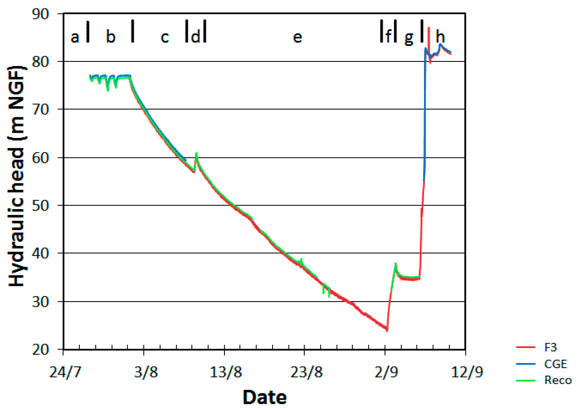
However, we also have to trust on the common sense of operators and analysts to “instinctively” avoid the most unstable periods for data collection. Thus, the conservative temperature assumption is unsuitable for runoff flow studies or all other kinds of events that imply transient and unstable thermal or water fluxes in the CS. This is why, the present work use a restriction of the White’s model to the recession period, with no run-off flow, and with a complete loss of the Upper Allogenic Stream (no surface stream). The 2005 Cent-Fonts pumping tests take place during the summer season when rainfalls are scarce on the watershed. However, even during that time, we focused the method on “steadiest” periods for water temperatures and flows. This is also why, despite available data until November, we stopped our analyses on 6 September (16:55) when a runoff due to a heavy thunderstorm flooded the boreholes (Figure 4).

3. Presentation of the Cent-Fonts Pumping Test Data

3.1. Period (a): Data Collected Prior the Beginning of the Pumping Test

Several years of flows and water temperatures have been recorded at the karst spring and in Buèges since 1997 to study the recession of the base flows during dry periods. This knowledge is essential to understand the answers of the aquifer during the pumping tests. The base flow (QS) gathers the upper allogenic intrusion of Buèges stream (QUAI) and the diffuse infiltration (QPFMB). The study of the karst recession conducted from 1997 to 2001 used a modified Mangin method to distinguish the parts played by QPFMB and QUAI to the base flow [23]. QS is described thank to three terms calculated from a Maillet homographic function [41]. Hence, two recession coefficients appear that characterizes the respective recession evolutions of QPFMB or QUAI. Ladouche et al. [23] calculated recession coefficients of 0.0080 (1998); 0.0088 (2000) and 0.0088 (day−1) (2001) for the QPFMB contribution to the base flow [23] (p. 64).
Complementary flows and water temperatures have been recorded in the weeks preceding the step-drawdown sequence on 27 July (see Table 1 for an accurate chronology of the pumping tests). Figure 4 presents the far field (T), the Upper Allogenic Intrusion (TUAI, Buèges), the Neighbor Allogenic Intrusion (TNAI, Hérault) and the CS (TCS, in Cge borehole) temperatures recorded from 1 July to 6 September. During the pumping tests, Cge’s devices provided CS hydraulic heads and temperatures until their disconnection by drawdown. TCS temperature was also recorded in the F3 borehole at the output of the pump (see Figure 2 and Figure 4).

3.2. Period (b): Data Collected during the Step-Drawdown Sequence (27 to 30 July)

Step-drawdown sequences are one of the most often performed pumping test to find out the behavior of wells and aquifer features. For the Cent-Fonts pumping test campaign, the pump has been placed directly inside a large CS conduit. The hydraulic heads recorded in F3, Reco and Cge will display such close curves they will be undistinguishable at the Figure 5 scale despite the bottleneck between Cge and F3 boreholes (Figure 2 and Figure 5). This superposition of curves reveals the hydraulic connectivity in this final part of the CS. Thus, the step-drawdown sequence will efficiently find out the resurgence yield by overestimating or underestimating the rate of pumping drying the spring.
Table 2 recalls the step-drawdown chronology, the pumping rates and the drying effects on griffons. QP of 0.2 and 0.3 m3/s did not achieve the completed drying of griffons while it was reached for 0.4 and 0.5 m3/s [26] (pp. 55–59). These results allow inferring that between 27 July and 30 July the base flow of the resurgence spring (that is QPFMB + QUAI) was ranging between 0.3 and 0.4 m3/s.
Four “coma-shaped” events (due to sudden deepening followed by recovering) occurred on the hydraulic head for each pumping of the step-drawdown sequence (Figure 5, Period (b)). During that time, the CS temperature remains constant to a few tens of degree while, on the opposite, TUAI (Buèges) and TNAI (Hérault) display diurnal temperature oscillations that reach 1 to 3 degrees (Figure 4). These diurnal temperature variations oscillate over 4 degrees, of meteorological trend that affect both TUAI and TNAI between 11 July and 30 July. The meteorological trend has the same amplitude on TUAI and TNAI. The amplitude of TUAI diurnal oscillations remains lower than those of TNAI because of shortness Buèges course and its low emergence temperature (12.5 °C). The stability of TCS despite these oscillations results from the damping effects of soils and 10 days underground transfer from the losses area to the Cent-Font resurgence [20].

3.3. Period (c): Constant High Rate Pumping (1 to 9 August)

Long high rate pumping is used to assess the answer of the aquifer to drawdown. From 1 August to 9 August, the hydraulic head in the CS increases linearly with time (note that to avoid concave curves in Figure 5, the data are not plotted versus the log of time as usual). However, the drawdown induces a reversal of the hydraulic head that triggers the intrusion of Hérault in the CS and a new contribution that adds to the base flow QPFMB coming from the PFM. Two new flows, QNAI and QPFMD are added to QPFMB and QUAI while spring drying let QP be the only discharge of the CS. During that time, TUAI and TNAI display diurnal and meteorological variations while T, recorded 25 m below the surface in the P7 borehole, remains remarkably constant (Figure 4, Period (c)).
TCS is recorded both in the Cge and F3 boreholes. The first is measured close to the arrival of the neighbor allogenic intrusion of Hérault (Figure 2). The second TCS is recorded deeper, close to the arrivals of QUAI and QPFMB. These two flows carry temperatures TUAI and T lower than this of TNAI. Thus, the values of the two TCS series diverge rapidly as soon as the drawdown triggers arriving of hot intrusive Hérault water in the CS branch near the Cge borehole. TCS (Cge recorded) increases rapidly a few hours after the starting of the high rate constant pumping from its 13.7 °C constant value since 2 August, 12h05. After a few days of transient evolutions, the temperatures in Cge and F3 boreholes stabilize respectively around 20 and 15 °C. Their temporal variations are correlated with the meteorological and diurnal trends observed for TNAI and TUAI (Figure 4, Period (c)).
The second series of TCS records (F3) stabilizes rapidly around 15 °C. It displays diurnal oscillating changes that are clearly due to the mixing of hot QNAI with the cold QPFMB, QPFMD and QUAI in the vicinity of the pump. This stabilization of the TCS increase indicates that QNAI acts like an almost constant vadose flow despite the increase of the hydraulic head between the water table and Hérault [26] (p. 191).
According to Maréchal et al. [34] we will considerer in the following the dewatering of the conduit network as a supplementary outgoing flow from the CS, QCS.

3.4. Period (d): Recovering Test (9 August)

The 6 h pump stop of 9 August allowed a recovering of 3.43 m (Figure 5, Period (d), and [26] (p. 65). During the interruption, QNAI brought warm water of Hérault that accumulated in the chimney above the pump. After pump re-starting, the temperature, TP displayed a short peak 9 August, 13h05 consecutive to the rapid extraction of this warm water. Similar phenomena occurred at the restarting 22 August, 13h30 and 3 September, 07h45 (Figure 4, Periods e and g).

3.5. Period (e): Constant High Rate Pumping (9 August to 2 September)

After 6 h of recovering, high rate pumping has been restarted from 9 August until 2 September. During Period (e), the hydraulic head decreased almost linearly with a slope similar to the one of Period (c). On 13 August at 12h15, the drawdown reached the level of the temperature probe in Cge borehole (51.6 m NGF), causing its disconnection and the loss of the TCS signal recorded there. At the end of Period (e), the drawdown approached the level of the pump in F3 that caused its stopping (Table 1).
As mentioned above for Period (c), two diurnal and meteorological trends are noticeable in the TNAI and TUAI temperature records. These variations are also present in the last part of TCS (Cge recorded) and in TCS (F3 recorded) (Figure 4, Period (e)).
From the beginning of August, the drawdown allowed speleological explorations of the resurgence branches (Figure 6). Surprisingly, while significant QPFMD infiltrations were expected in CS, no water was apparently percolating through the chimney wall (Figure 6a–c). However, several cascading vadose flows were observed between marks 657–658 of the lifeline (Figure 6d) and mark 670 (Figure 6e). Partial catchments of these Hérault intrusions at point 657 collect 0.045 to 0.050 m3/s [26] (p. 40). This value gives a rough lower bound value of QNAI since other hidden or deeper entries were probably active. These speleological explorations also opened the opportunity to collect geochemical samples to quantify the mixing of Hérault intrusion in the CS.
Water samples were collected 1 September at the above intrusion points. We used PP® bottles previously washed with chlorydric acid, then bromydric acids, to prevent contamination [42]. Bottles and corks have been rinsed four times on site. The solutions have been filtered, acidified and prepared in two dilutions for analysis. Complementary samples were collected the same day at the Buèges spring, in Hérault and at the pump.
The samples were analyzed for the Rb, Sr, and Ba on the VG Plasmaquad II turbo ICPMS of Montpellier 2 University (Table 3 and Figure 7). Sr, Rb, and Ba have been chosen as field tracers for water circulation and mixing [4] Petelet et al. 2003). Figure 7 shows the alignment of the samples in a (Ba/Sr) vs. (Rb/Sr) graph. The alignment of point denotes a mixing between two poles [43]. According to the regression curves and the rate of pumping QP = 0.4 m3/s, QNAI ranges from 0.039 to 0.048 m3/s for Ba, from 0.060 to 0.083 m3/s for Sr, and from 0.077 to 0.087 m3/s for Rb. However, the lower values of the Ba/Sr ratio may reflect a sorption effect onto mineral-water interfaces [44]. The averaged value of these six measures gives QNAI = 0.066 m3/s.

3.6. Period (f): Recovering Test (2 September to 3 September)

A second stop of the pump lasts 24 hours and 25 minutes, from 2 September to 3 September, that induced a 13.49 m recovering in the chimney (Figure 5).

3.7. Period (g): Drawdown Constant Pumping (3 September to 6 September)

The equilibrium-pumping (Period (g)) followed one month of constant pumping at constant rate that resulted in an important drawdown. After the recovering of Period (f), the equilibrium-pumping aimed to assess the dynamics of aquifer answer to hydraulic head. It started on 3 September at 7h45 with QP = 0.324 m3/s. The pumping rate has been dropped to QP = 0.304–0.305 m3/s a few hours later to stabilize the hydraulic head at 35.0 ± 0.1 m NGF (Figure 5).
Since, this value is around 40 m deeper than the karst base level the Hérault intrusion remained active (the first intrusion of Hérault occurred for 76.7 m NGF on 1 August at 07h10).

4. Revisiting the 2005 Pumping Test Data

The challenge of studying temperature as a conservative tracer also faces the natural complexity of karsts, which CS mixes water coming from low resistance conduits and low permeability PFM. A few decades ago, studies were often considering medium where CS was not disrupting the aquifer but continuous models were unsatisfactorily. Since a few years, improved analytical models take better into account for the different behavior of the two types of reservoirs [34] or even three reservoirs [45]. However, despite the importance of calibration for the models, temperature has not been used probably because of the non-conservative character of this signal [26,34]. In the following we will take benefit of particular periods of the pumping test to get new constraints for the models.
Our process consists, firstly, to revisit the data of Period (a) to recalculate the base flow QPFMB that forms the background over which the assessment of QPFMD is possible. Secondly, we benefit of the base flow knowledge to reevaluate the intrusion of Hérault, QNAI, on Period (g). Thirdly, relying on QPFMB and QNAI, we re-assess QPFMD, the answer of the aquifer to drawdown, during the constant pumping (Periods (c) and (e)).

4.1. Revisiting QPFMB from Period (a)

4.1.1. Revisiting the Data

Unlike Maréchal et al. [34], but following the results of [26] (p. 64), we consider that the recession of the Cent-Fonts base flow is better described separating the Buèges contribution QUAI. Then, the recession of QPFMB is calculated using Equation (11) in which we need to set the amplitude coefficient QPFMB(to).
Q P F M B ( t ) = Q P F M B ( t 0 ) e 0.0088 ( t t 0 )
Without pumping, the only flow leaving the CS is the one of the spring. In July 2005, as the surface course of Buèges fully disappears, and since no pumping affects the resurgence, no drawdown occurs in the CS. Under these natural conditions QS gathers QUAI and QPFMB and the water table in CS sits on top of the base level by a few centimeters. This weak hydraulic head is enough to prevent Hérault to intrude.
Then, replacing qk = QPFMB, Tk = T, ql = −QS, Tl = TCS, qi = QUAI and Ti = TUAI in Equation (8) leads to the Equation (12) below where the spring discharge QS and the base flow QPFMB are unknowns.
Q P F M B = Q U A I ( T U A I T C S ) ( T C S T ) Q S = Q P F M B + Q U A I
It is, therefore, possible to fix QPFMB(to) in the recession curve with the values QUAI, TUAI, TCS and T recorded for several weeks. 
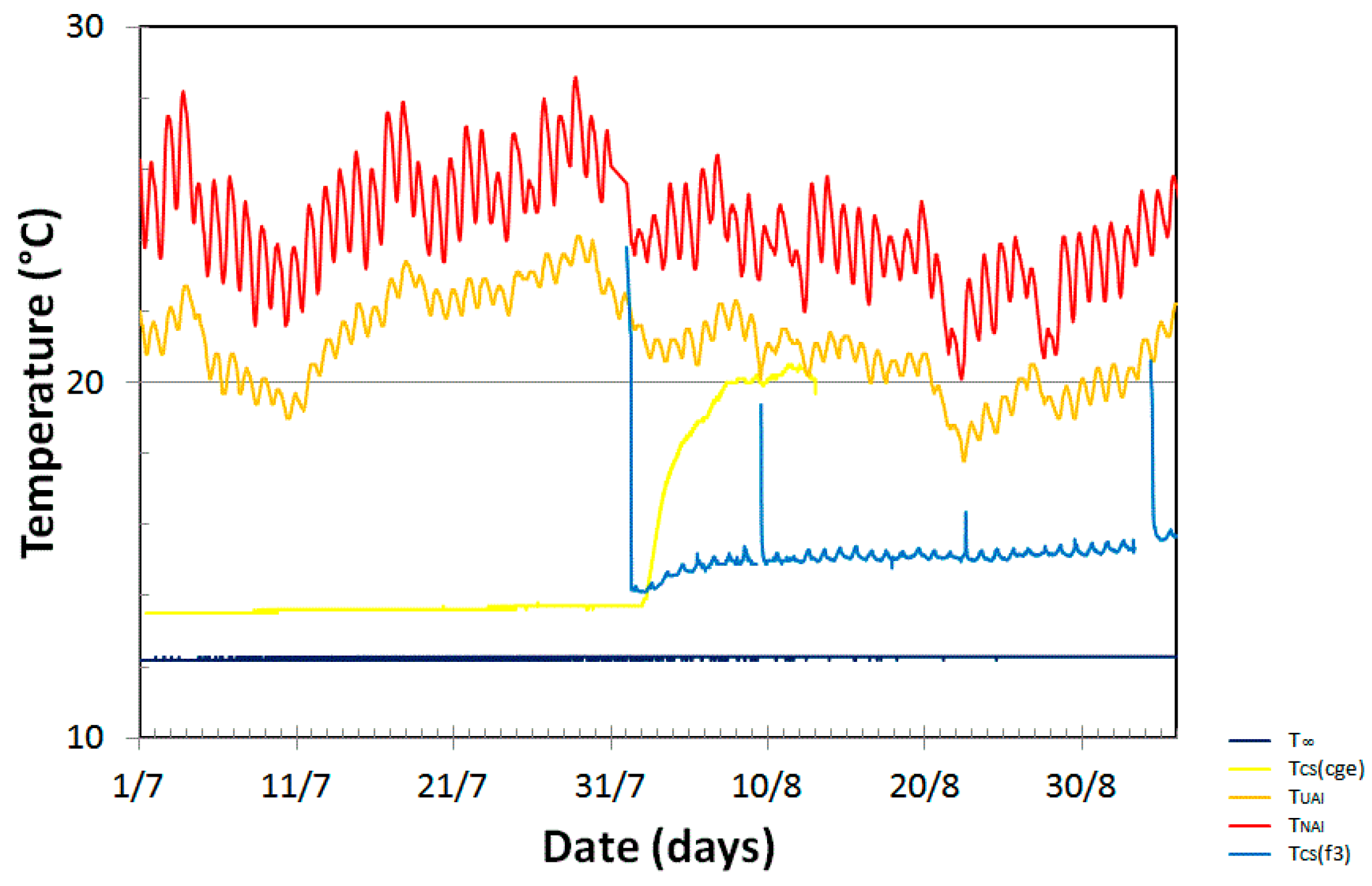
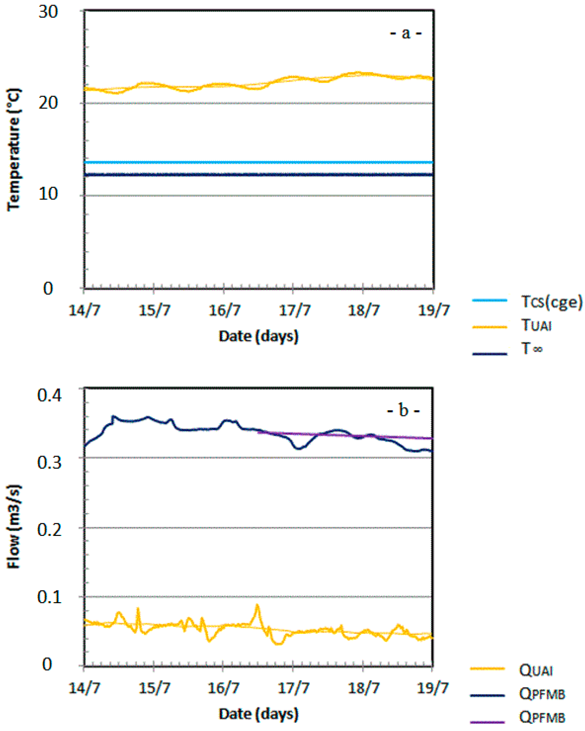
Figure 8 displays an enlargement of these records from 14 July (00:00) to 19 July (23:55). TUAI displays diurnal oscillations of 0.2 to 0.4 °C around its 24-h moving averaging and a small meteorological increasing trend of a few degrees (Figure 8, top). In bottom panel of Figure 8, QUAI also displays diurnal oscillations due to the water catchments upstream of the swallow zone. Concurrently, T and TCS remain remarkably stable (Figure 8, top). The QPFMB curve in the bottom panel of Figure 8 displays the results of Equation (12) solving. We calculated its mean values (0.336 m3/s) and affected it at the median time to = 16 July (12:00) to extrapolate the PFM base flow for the remainder of our study (Equation (13)).
Q P F M B ( t ) = 0.336 e 0.0088 ( t t 0 )

4.1.2. Assessment of Error Due to Data Variability

Two kinds of inaccuracy may affect the measures and, therefore, the use of QUAI, TUAI, TCS and T for the method described in this article. The first are the precisions of the measures while the second relate to the difference between the steady state and the physical conditions in the CV. In the following, we will consider that modern thermometers result in negligible errors (less than 0.1 °C) in front of those resulting of unsteady behaviors. For Buèges gauging, the level error δQUAI at the swallow zone is not explicitly mentioned [26]. However, it is reduced by the total swallowing that limits it to the one of the zone entry. It is also reduced by the low flow context that allows more accurate gauging [46]. Therefore, without better assessment of this error, it seems reasonable to consider that it remains lower than a few liters by second. This level matches the one of standard errors induced by the diurnal variations (Table 4).
Equation (10) provides a powerful tool to assess how errors spread through the solving. According our preceding comments, and considering the stability of TCS and T, we have reported δT = 0 and δTCS = 0 in Equation (10). The differential form of Equation (9) becomes Equation (14), for which the numerical coefficients have been calculated by using the mean values and the Standard Errors of temperatures and flows.
δ Q P F M B = 1 ( T C S T ) [ ( T U A I T ) δ Q U A I + Q U A I δ T U A I ] δ Q S = δ Q P F M B + δ Q U A I δ Q P F M B = 6.21 δ Q U A I + 0.038 δ T U A I
More realistic physical conditions have been searched for in the CS by operating 24-h moving averaging on the diurnal variations of raw data (Table 4, columns 6 and 8). Such numerical process accounts for the natural thermal and kinetic inertia acting along underground water flows and allows damping the error that could arise from their neglecting. Thus, over a few days, a meteorological trend increases the temperature recorded at the Buèges swallow zone by one to two °C (Figure 8). However, the final standard error remain limited to 0.64 °C on raw data (Table 4, column 6) and to 0.55 °C after 24-h averaging of the data (Table 4, column 8). The natural damping of temperature fluctuations that affects QUAI during its underground travel to the CS prompts to consider the standard error as an upper bound.
Equation (14) shows that 1 °C of error on TUAI induces 38 L/s (liters by second) of error on QPFMB; and that one L/s of error on QUAI induces 7 L/s on the final result. We can therefore expect that QPFMB is obtained to a few tens of L/s (around 20%) (Table 4, columns 7 and 9). This is consistent with the step drawdown tests that revealed a spring flow QPFMB + QUAI comprised between 0.3 and 0.4 m3/s.

4.1.3. Assessment of Error due the Conservative Temperature Assumption

Another way to explore the effects of non-stationarity on the solutions consists in confronting karst numerical models that consider (or not) temperature as a conservative tracer. This has been done in a previous study where several numerical models have been calculated over very broad ranges of karst morphological and hydrological parameters. According to Equation (15) of [36] a first order of the error induced by the conservative temperature assumption is reached by the following Equation (15):
δ T = ε [ ( T C S + T ( T U A I T ) ) ]
The error, ε’, is calculated versus the hydrological and morphological properties as thermal diffusivity ratio (9.93), Conduit Peclet number (1.5 × 10⁸), Prandtl number (6.99) and Conduit Reynolds number (4.29 × 10⁴). Table 1 and Table 5 recall the form and the physical values compatible with the Cent-Fonts karst. Then, the abacus curves of Figure 4 of [36] indicate ε’ = 0.00613 at the exit of the CS. With ε’ = 0.00613, TCS = 286.75 K, TUAI = 295.45 K and T = 285.35 K (Table 4, Period (a)) the first order of the error δT = 1.93 °C. Coming back to Equation (14), we can see that it may induce 0.073 m3/s of error for QPFMB. This result is higher but remains consistent with the previous estimate and the results of the step drawdown tests.

4.2. Revisiting QNAI from Périod (g)

4.2.1. Revisiting the Data

As recalled above, the equilibrium-pumping that started on 3 September (7h45) and ended on 6 September (6h00) followed one month of constant pumping and a one day recovering. After a few hours, the initial rate QP = 0.324 m3/s has been lowered to QP = 0.304–0.305 m3/s that stabilized the hydraulic head at 35.0 ± 0.1 m NGF (Figure 5). This hydraulic head is around 40 m deeper than the base level Hérault. Consequently, the Hérault intrusion QNAI remained fully active during all the equilibrium-pumping.
During Period (g), the incoming flows in the CS are QUAI, QNAI and both basic and drawdown induced PFM contribution QPFM = QPFMB + QPFMD. These input flows equilibrate the output flow QP while the stabilization of the hydraulic implies that the dewatering of the CS stops (QCS = 0). Hence, Equation (9) can be rewritten as Equation (16) to calculate QNAI, and QPFM.
Q N A I = Q P ( T P T ) Q U A I ( T U A I T ) ( T N A I T ) Q P F M = Q P ( T N A I T P ) Q U A I ( T N A I T U A I ) ( T N A I T )
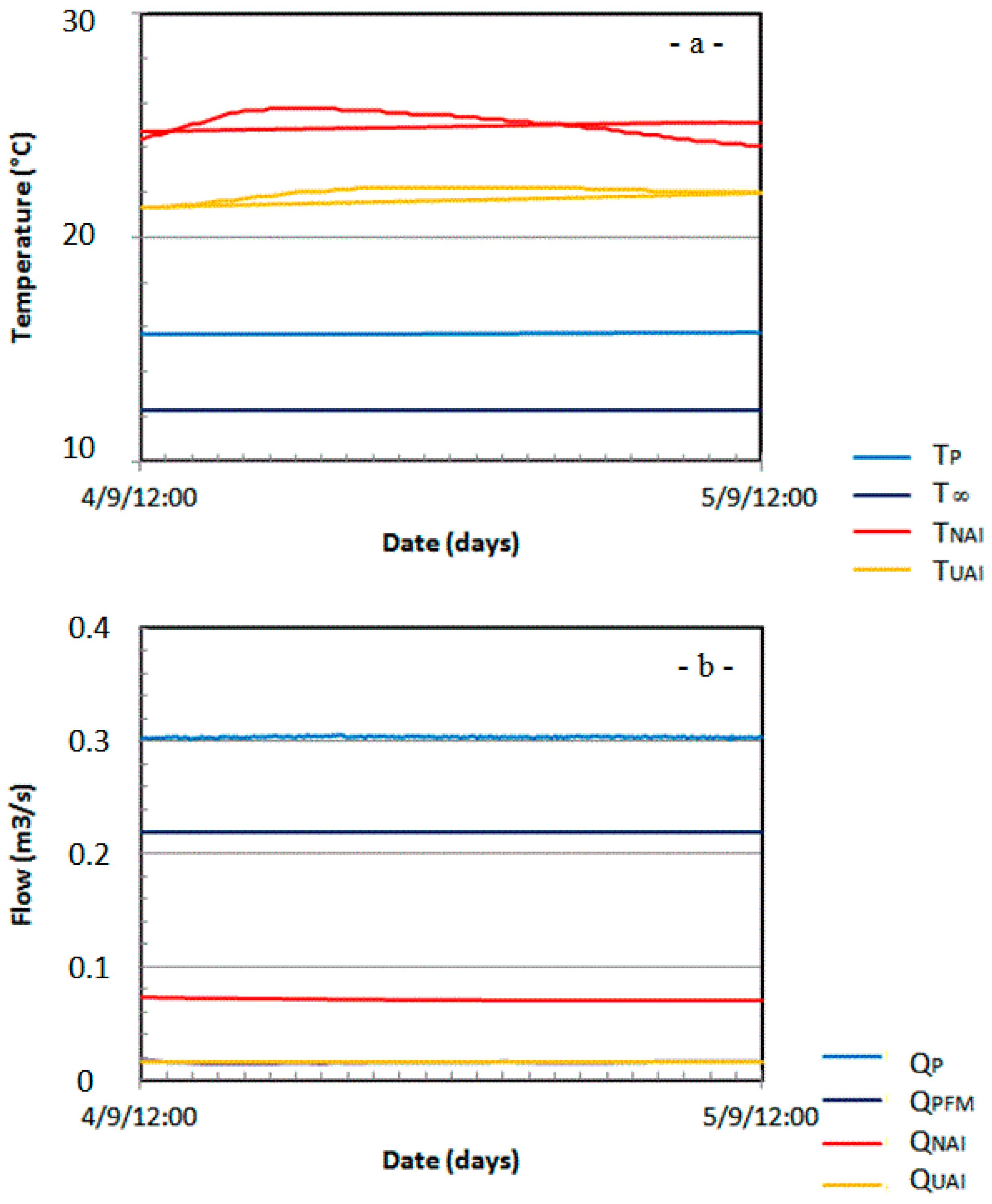
We focus on a remarkably stable 24-h data range from 4 September (12:00) to 5 September (12:00) (Figure 9). Indeed, the sinusoidal shapes of TUAI and TNAI are fully damped by the 24-h moving averaging, while T, TP, and QUAI remain rather constant.
The bottom panel of Figure 9 displays the results obtained for QNAI and QPFM. They lead to mean values of QNAI = 0.070 m3/s and QPFM = 0.219 m3/s. The first agrees well with the geochemical results presented in Section 3 while the second is only a few L/s higher than the base flow QPFMB = 0.216 m3/s obtained from Equation (11) for t = 5 September (00:00). This seems indicate that, a few hours after stabilization of the hydraulic head, the PFM contribution due to drawdown, QPFMD, is very low.

4.2.2. Assessment of Error Due to Data Variability

A procedure similar to the one described in Period (a) has been applied to Period (g) assessing the error due to data variability. The mean values of the parameters obtained on this interval have been introduced in the reduced form of Equation (10) to calculate the propagation of these errors through the resolution process (Equation (17)).
δ Q N A I = 1 ( T N A I T ) 2 [ ( Q U A I ( T U A I T ) Q P ( T P T ) ) δ T N A I δ Q U A I ( T U A I T ) ( T N A I T ) Q U A I ( T N A I T ) δ T U A I ] δ Q N A I = 0.0056 δ T N A I 0.760 δ Q U A I 0.0012 δ T U A I δ Q P F M = 0.0056 δ T N A I 0.240 δ Q U A I + 0.0012 δ T U A I
In this analysis, we will consider that pump gauging error δQP is negligible in front of δQUAI. Equation (17) shows that 1 °C of error on TNAI induces 5.6 L/s of error on QNAI or QPFM; that of 1 L/s on QUAI results in 0.760 L/s; and that 1 °C on TUAI induces 1.2 L/s. When the standard error of Table 4 are introduced in Equation (17), the error falls to a few L/s (a few %) (Table 4, Period (g)).

4.2.3. Assessment of Error Due the Conservative Temperature Assumption

During the equilibrium pumping, but also during constant pumping, most of the CS mixing occurs near the pump, in the top part of the chimney just beside Hérault (Figure 2). This proximity causes the diurnal oscillation of TP that occur with a delay of 20 h (Figure 4). The drawdown changes significantly the configuration of the CV with a mixing zone close to Hérault. The distance between the river and the chimney that contains the pump is less than 200 m. We have to take these consequences of the drawdown to assess the error due to the conservative temperature approximation during heavy pumping. Therefore, using these delay and distance to estimate the properties of the CV, the CS Peclet number and the Conduit Reynolds number fall respectively to Pe = 3.9 × 10⁶ and Re = 2.78 × 10⁴ (Table 5). The ratio of (PFM to Water) thermal diffusivities and the Prandtl number remain unchanged. We will use this new dimensionless configuration revisiting the data on Periods (e) and (g). (With these new values the abacus curves of Figure 4 of [36] tell that ε’ reaches around 0.002 at the exit of the CS.
δ T = ε [ ( T P + T ( T N A I T ) ) ]
With ε’ = 0.002, TP = 288.88 K, TNAI = 298.25 K and T = 285.35 K (Table 4, Period (g)) δT reaches 0.62 °C. Through Equation (17), it induces a 0.003 m3/s error for QPFM. Similarly to the comparison of error on Period (a), both methods of error assessment lead to consistent results.

4.3. Revisiting QPFMD from Period (e)

4.3.1. Revisiting the Data

The knowledge of QPFMB and QNAI makes possible a backward analysis of the data recorded during Periods (c) and (e). Indeed, QPFMB forms the background over which it is possible to assess QPFMD. On the other hand, the vadose character of the Hérault intrusion results in a constant amplitude despite an increasing drawdown [26] (p. 191). These two previous results bring two “corner stones” situations separated by the constant pumping sequence. This allows us calculating two unknown flows: QPFM that includes the drawdown induced contribution QPFMD and the dewatering of the CS (QCS). The linear increase of the hydraulic head with time over Periods (c) and (e) (Figure 5) suggests a constant dewatering rate, bolstering us to assume a near steady CV situation. The input flows are QUAI, QNAI, QPFMB, QPFMD and the output flows are QCS and QP.
In order to maintain these “constant” conditions at best, our data processing skipped the data 24 h before and after the stopping. This allowed avoiding the transient phenomena observed at the restarting of the pump for temperature (Figure 4) and discharges. Consequently, we focused our analysis from 10 August (00:00) to 1 September (19:10). Within the context, Equation (9) can be rewritten as Equation (17).
Q P F M = Q P ( T P T C S ) Q U A I ( T U A I T C S ) Q N A I ( T N A I T C S ) ( T T C S ) Q C S = Q P ( T T P ) Q U A I ( T T U A I ) Q N A I ( T T N A I ) ( T T C S )
The brutal increase of the temperature records in the Cge borehole shows that, as soon as Hérault intrudes through the horizontal shallow branch of the CS, TCS(Cge) is less representative of the dewatering temperature TCS. Therefore, we will alternatively consider that the temperature recorded at the pump may represents another assessment TCS(f3). This assumption seems reasonable since TCS(f3) is only a few degrees higher than the TCS temperature obtained on Period (a) before the mixing with the hot Hérault water.
The results of calculations for QPFM and QCS are presented on the lower diagram of Figure 10. From QPFM and QPFMB (Equation (13)), it is easy to calculate QPFMD. For both TCS(Cge) and TCS(f3) assumptions, QPFMD(Cge) and QPFMD(f3) curves display diurnal oscillations but do not display clear increasing trends despite of drawdown deepening. Figure 10 shows that QPFMD(Cge), QPFMD(f3), QCS(Cge) and QCS(f3) are clearly affected by the diurnal and meteorological oscillations on QNAI and QUAI. Considering the most advantageous situation TCS(Cge), QPFMD ranges between 0.030 and 0.050 m3/s. However, this drawdown induced contribution is probably overestimated because of a too hot dewatering temperature assumption TCS. Indeed, the calculation forces the system to equilibrate on the pump temperature. This will increase the low temperature contribution QPFM at the expense of the hot dewatering QPFM. On the other hand QPFMD(f3), computed taking the pump temperature as TCS seems really too low since it would induces a zero or even negative contribution of QPFM to drawdown. In any case, these results seem consistent with short transient flows coming with the increase of the hydraulic head. These conclusions are consistent with the ones of Maréchal et al. [34], and consistent with the shortness of the flows observed at the beginning of the equilibrium-pumping phase.

4.3.2. Assessment of Error Due to Data Variability

Following the same procedure, the mean values of the parameter over this interval (Table 4—Period (e)) have been introduced into the reduced form of Equation (10) to establish the formal and numerical forms of Equation (20).
δ Q P F M = 1 ( T C S T ) 2 [ δ T C S ( Q P ( T P T ) Q U A I ( T U A I T ) Q N A I ( T N A I T ) ) δ Q U A I ( T U A I T C S ) ( T T C S ) δ T U A I Q U A I ( T T C S ) δ Q N A I ( T N A I T C S ) ( T T C S ) δ T N A I Q N A I ( T T C S ) ] δ Q P F M = 0.0044 δ T + 0.039 δ Q U A I + 0.0024 δ T U A I + 0.447 δ Q N A I + 0.0092 δ T N A I δ Q C S = 0.0044 δ T 1.289 δ Q U A I 0.0024 δ T U A I 1.697 δ Q N A I 0.0092 δ T N A I
One °C of error on TCS value induces 4.4 L/s of error for QPFM. Finally, 1 °C of error on TUAI induces 2.4 L/s of error and one °C on TNAI results in 9.2 L/s of error. The introduction of the Standard error (24SE—Table 4) in Equation (20) leads to 14 to 21 L/s of error on QPFM and on QCS. Thus, small amplitude of QPFMD makes the error is of the same order than QMCD itself.

4.3.3. Assessment of Error due to the Conservative Temperature Assumption

As mentioned above, we consider that the hydrological configuration induced by drawdown is the same the one of Period (g). Then, the CS Peclet number and the Conduit Reynolds number remain the same and, ε’ keeps the same value around 0.002 at the exit of the CS.
δ T = ε [ ( T P + T ( T N A I T ) ) ]
Therefore, the error on temperature balance due to the conservative approximation δT remains of the order 0.62 °C. Such temperature error would induce several tens liters by second of errors.

5. Summary and Discussion

The heat and matter exchanges occurring through the karstic boundaries impose a consideration of the Open Thermodynamic System (OTS). Within this framework, the first principle of thermodynamics leads to an enthalpy balance between flows entering and leaving the CV. Combining this property with mass conservation leads to systems of two equations involving the flows and temperatures. If formal physical conditions (steady states) are never achieved in nature, they are approached during particular periods as recession or certain phases of the pumping tests. These periods have been used these to calculate “corner stones” descriptions of the hydraulic regime between which we extend the results. The restriction of our model to the quietest part of the recession period cuts off the risk of disruption an approximate steady state by flooding and the possibility of reverse flow from CS to PFM. That way the periods of data revisiting were chosen outside of the recovering and the analysis has been stopped as soon as the flood event of 6 September occurred.
Revisiting the data recorded during these three periods with our theoretical analyses leads to a recalculation of consistent hydrological behavior of the karstic system. Thus, the speleological, hydrological or geochemical observations validated by previous studies [26,34] are not refuted despite of a less optimistic yield of the resurgence. This is particularly the case for spring drying during the step drawdown sequence, the results of geochemical analyses or the base flow recession of the resurgence.
Even though it is never perfectly reached in nature, the steady state approximation is necessary to use the method. While such state is assumed, temperatures equilibrate at the PFM/Conduit interface. However, this situation does not mean cancelling of embedding rocks/water heat transfer at the interface. Indeed, as shown in Machetel and Yuen 2015, PFM temperature gradient is maintained by the advection of cold, far field, water that counteracts the heat diffusion from CS to PFM through the wall. During the recession period, mixing of intrusive flows hotter than far field temperature, results in CS temperature hotter than in PFM. However, when a steady state is reached (or approached), all these local conductive effects (inside PFM and CS but also between PFM and CS) are taken into account by the final enthalpy balance. This is the most interesting property of the OTS approach that refers to the comparison of integrated incoming and leaving external heat sources and not on the local thermal properties inside of the “black box”. It is clear that what we called “conservative temperature assumption” may better be called as “conservative enthalpy approximation”. However since we assumed that no other sources of heat are present (neither chemical heat, nor work conversion to heat); enthalpy conservation comes down on to temperature conservation.
Thus, the application of the method to the first period (before pumping) of the Cent-Fonts pumping test experiments allowed assessing the basic recession flow of the resurgence. Then, the equilibrium-pumping allowed assessing the Hérault intrusion and the supplementary contribution induced by drawdown. The analysis shows that errors induced by unsteadiness reach a few tens of liters by second. They are of the same order of magnitude than the errors induced by conservative approximation itself.
In conclusion, we have confirmed the validity for using the thermometric method by the field observations that never contradict the results. It would be advantageous; insofar data exists, to check the method on other sites. It could also be interesting and of relatively low additional costs to develop recording and processing of temperature profiting of next pumping experiments. Indeed, as it does not require sophisticated equipment or procedures, the additional costs should remain low compared to drilling and pumping operations.
Our works may open the opportunity of using the steadiest part of the pumping test sequences to calibrate the global operating mode of complex resurgence system. Combining energy equation and mass conservation equations, temperature measurements in surface waters and boreholes may allow assessing the flow properties in borehole or mixing in karst CS. It seems therefore constitute an efficient tool to separate and calculate the karstic properties and could be a promising tool worthwhile to apply on other sites.

Acknowledgments

The authors thank “le Conseil Général de l’Hérault” and the PREVHE association for providing the complete set of digital data of the 2005 Cent-Fonts pumping test campaign and financing ICPMS analyses. We also thank Jean-Marc Luck and Olivier Bruguier for their active participation to the analysis of water samples on the ICPMS “Turbo PQ2 Quadruple Plasma VG Plus” of Montpellier University and their interpretation. We also thank the two anonymous referees, which comments contributed to improve this paper. This work benefited of a grant from China University of Geosciences.

Author Contributions

Philippe Machetel and David Yuen are both involved in numerical solving of non-linear differential equations, thermodynamics and physics of fluids.

Conflicts of Interest

The authors declare no conflict of interest.

Appendix A

A.1. Acronyms

CSConduit System of fluviokarstic system
CVControl volume of the OTS
OTSOpen Thermodynamic System
PFMPorous Fractured Matrix

A.2. Cent-Fonts Fluviokarst Flows, White’s and Pumping Test Notations

A.2.1. CS Inflows (m3/s)

QUAIUpper allogenic stream intrusion (Buèges intrusion at swallow zone—M)
QNAINeighbor allogenic stream intrusion (Hérault intrusion at base level—C)
QPFMPorous Fractured Matrix to CS flow (C)
QPFMBPorous Fractured Matrix to CS base flow (C)
QPFMDPorous Fractured Matrix to CS drawdown induced flow (C)
QDDrawdown induced Porous Fractured Matrix to CS flow (C)

A.2.2. CS outflows (m3/s)

QSSpring discharge (Resurgence discharge in Hérault M or C)
QPPump discharge (Pump discharge in Hérault during pumping tests—M)
QCSCS Dewatering corresponding to the lowering of water table (C)

A.2.3. Temperatures (°C)

TUAIUpper allogenic stream temperature (M)-Buèges temperature (M)
TNAINeighbor allogenic stream temperature (M)-Hérault temperature (M)
TPPump output temperature (M)
TCSCS water temperature (C or M)
TFar field temperature-P7 borehole temperature (M)

A.3. Equations Notations (units)

vFluid velocity vector(m/s)
qiCS algebraic value (positive for incoming flow)(m3/s)
qoCS algebraic value (negative for outgoing flow)(m3/s)
δECS Internal Energy(J)
jCS incoming or outgoing flows(-)
hjSpecific enthalpy of CS flow j(J/kg)
epot,jPotential energy of CS flow j(J/kg)
ecin,jKinetic energy of CS flow j(J/kg)
δΦjCS-PFM Thermal exchanges(J)
δWjCS-PFM Work exchanges(J)
ρjWater density in flow j(kg/m3)
CpjSpecific thermal capacity in flow(J/kg K)
TiTemperature of CS incoming flow(°K or °C)
ToTemperature of CS incoming flow(°K or °C)

A.4. Error Assessment Notations, (Units), Values

DmPFM thermal diffusivity(m2/s)1.42 × 10−6
DwWater thermal diffusivity(m2/s)1.43 × 10−7
υWater kinematic viscosity(m2/s)10−6
LCS Length(m)5 × 10³
rhHalf hydraulic radius(m)5
VVelocity scale(m/s)
DThermal diffusivity ratio (Dm/Dw)(-)
PeConduit Peclet number (LV/Dw)(-)
PrPrandtl number (υ/Dw)(-)
RedCS Reynolds number (2 V·rh)/υ(-)
δTConservative hypothesis error(C or K)

References

  1. Constantz, J. Interaction between stream temperature, streamflow, and groundwater exchanges in Alpine streams. Water Resour. Res. 1998, 34, 1609–1615. [Google Scholar] [CrossRef]
  2. Constantz, J. Heat as a tracer to determine streambed water exchanges. Water Resour. Res. 2008, 44, 2008. [Google Scholar] [CrossRef]
  3. Tabbagh, A.; Bendjoudi, H.; Benderitter, Y. Determination of recharge in unsaturated soils using temperature monitoring. Water Resour. Res. 1999, 35, 2439–2446. [Google Scholar] [CrossRef]
  4. Benderitter, Y.; Roy, B.; Tabbagh, A. Flow characterization through heat transfer evidence in a carbonate fractured medium: First approach. Water Resour. Res. 1993, 29, 3741–3747. [Google Scholar] [CrossRef]
  5. Genthon, P.; Bataille, A.; Fromant, A.; D’Hulst, D.; Bourges, F. Temperature as a marker for karstic waters hydrodynamics. Inferences from 1 year recording at La Peyrere cave (Ariège, France). J. Hydrol. 2005, 311, 157–171. [Google Scholar] [CrossRef]
  6. Genthon, P.; Wirrmann, D.; Hoibian, T.; Allenbach, M. Steady water level and temperature in a karstic system: The case of the coral Lifou Island (SW Pacific). C. R. Geosci. 2008, 340, 513–522. [Google Scholar] [CrossRef]
  7. Karanjac, J.; Altug, A. Karstic spring recession hydrograph and water temperature analysis—Oymapinar Dam Project, Turkey. J. Hydrol. 1980, 45, 203–217. [Google Scholar] [CrossRef]
  8. Stonestrom, D.A.; Constantz, J. Using temperature to study stream-ground water exchanges. US Geol. Surv. Fact Sheet 2004, 3010, 4. [Google Scholar]
  9. O’Driscoll, M.A.; DeWalle, D.R. Stream-air temperature relations to classify stream-ground water interactions. J. Hydrol. 2006, 329, 140–153. [Google Scholar] [CrossRef]
  10. Mosheni, O.; Stefan, H.G. Stream temperature/air temperature relationship: A physical interpretation. J. Hydrol. 1999, 218, 128–141. [Google Scholar] [CrossRef]
  11. Bogan, T.; Mosheni, O.; Stefan, H.G. Stream temperature-equilibrium temperature relationship. Water Resour. Res. 2003, 39, 1245. [Google Scholar] [CrossRef]
  12. Bogan, T.; Stefan, H.G.; Mosheni, O. Imprints of secondary heat sources on the stream temperature equilibrium temperature relationship. Water Resour. Res. 2004, 40, W12510. [Google Scholar] [CrossRef]
  13. Sinokrot, B.A.; Stefan, H.G. Stream temperature dynamics measurements and modeling. Water Resour. Res. 1993, 29, 2299–2312. [Google Scholar] [CrossRef]
  14. Luetscher, M.; Jeannin, P.Y. Temperature distribution in karst systems: The role of air and water fluxes. Terra Nova 2004, 16, 344–350. [Google Scholar] [CrossRef]
  15. Dogwiller, T.; Wicks, C. Thermal variations in the hyporheïc zone of a karst stream. Int. J. Speleol. 2006, 35, 59–66. [Google Scholar] [CrossRef]
  16. Petelet, E.; Luck, J.M.; Ben Ohtman, D.; Negrel, P.; Aquilina, L. Geochemistry and water dynamics of a medium-sized watershed: The Hérault, southern France 1. Organization of the different water reservoirs as constrained by Sr isotopes, major, and trace elements. Chem. Geol. 1998, 150, 63–83. [Google Scholar] [CrossRef]
  17. Dubois, P. Étude des réseaux souterrains des rivières Buèges et Virenque (le Languedoc Bas). In Proceedings of the 2e Congrès International de Spéléologie, Salerne, Italy, 2–12 October 1958.
  18. Paloc, H. Carte Hydrogéologique de la France, Région Karstique Nord-Montpelliéraine, Notice Explicative; Bureau de Recherches Géologiques et Minières: Orléans, France, 1967.
  19. Camus, H. Formation des réseaux karstiques et creusements des vallées: L’exemple du Larzac méridional, Hérault, France. Karstologia 1997, 29, 23–42. [Google Scholar]
  20. Schoen, R.; Bakalowicz, M.; Ladouche, B.; Aquilina, L. Caractérisation du Fonctionnement des Systèmes Karstiques Nord-Montpelliérains. Rap. BRGM R40939RP. 1999, Volume III, p. 91. Available online: http://infoterre.brgm.fr/rapports/RR-40939-FR.pdf (accessed on 27 November 2016).
  21. Aquilina, L.; Ladouche, B.; Bakalowicz, M.; Schoen, R.; Petelet, E. Caractérisation du Fonctionnement des Systèmes Karstiques Nord-Montpelliérains. Synthèse Générale. Rap. BRGM R40746. 1999, p. 50. Available online: http://infoterre.brgm.fr/rapports/RR-40746-FR.pdf (accessed on 27 November 2016).
  22. Petelet-Giraud, E.; Dörfliger, N.; Crochet, P. RISK: Méthode d’évaluation multicritère de la vulnérabilité des aquifères karstiques. Application aux systèmes des Fontanilles et Cent-fonts (Hérault, sud de la France). Hydrogéologie 2000, 4, 71–88. [Google Scholar]
  23. Ladouche, B.; Dörfliger, N.; Pouget, R.; Petit, V.; Thiery, D.; Golaz, C. Caractérisation du Fonctionnement des Systèmes Karstiques Nord-Montpelliérains, Rapport du Programme 1999–2001. Buèges, Rap. BRGM 51584 Fr RP. 2002. Available online: http://infoterre.brgm.fr/rapports/RP-51584-FR.pdf (accessed on 27 November 2016).
  24. Petelet-Giraud, E. Dynamic scheme of water circulation in karstic aquifers as constrained by Sr and Pb isotopes. Application to the Hérault watershed, Southern France. Hydrogeol. J. 2003, 11, 560–573. [Google Scholar] [CrossRef]
  25. Aquilina, L.; Ladouche, B.; Dörfliger, N. Recharge processes in karstic systems investigated through the correlation of chemical and isotopic composition of rain and spring-waters. Appl. Geochem. 2005, 20, 2189–2206. [Google Scholar] [CrossRef]
  26. Ladouche, B.; Maréchal, J.C.; Dörfliger, N.; Lachassagne, P.; Lanini, S.; Le Strat, P. Pompage D’essai sur le Système Karstique des Cent-Fonts (Commune de Causse de la Selle, Hérault), Présentation et Interprétation des Données Recueillies. Rap. BRGM RP54426-FR. 2005. Available online: http://infoterre.brgm.fr/rapports/RP-54426-FR.pdf (accessed on 27 November 2016).
  27. Aquilina, L.; Ladouche, B.; Dörfliger, N. Water storage and transfer in the epikarst of karstic systems during high flow periods. J. Hydrol. 2006, 327, 472–485. [Google Scholar] [CrossRef]
  28. Elguero, E. Les Grandes Cavités Héraultaises; A.V.L. Diffusion: Montpellier, France, 2004; p. 44. [Google Scholar]
  29. Smart, C.C. A deductive model of karst evolution based on hydrological probability. Earth Surf. Process. Landf. 1988, 13, 271–288. [Google Scholar] [CrossRef]
  30. Malcom, A. Lexicon of Cave and Karst Terminology with Special Reference to Environmental Karst Hydrology. Supercedes EPA/600/R-99/006, 1/’99; National Center for Environmental Assessment, Office of Research and Development, U.S. Environmental Protection Agency: Washington, DC, USA, 2002; p. 214.
  31. White, W.B. Karst hydrology: Recent developments and open questions. Eng. Geol. 2002, 65, 85–105. [Google Scholar] [CrossRef]
  32. White, W.B. Conceptual models for karstic aquifers. Speleog. Evol. Karst Aquifers 2003, 1, 6. [Google Scholar]
  33. Jambac, F. Essais Complémentaire sur le Site des Cent-Fonts; Technical repport; Compagnie Générale de Eaux: Montpellier, France, 1994. [Google Scholar]
  34. Maréchal, J.C.; Ladouche, B.; Dörfliger, N.; Lachassagne, P. Interpretation of pumping tests in a mixed flow karst system. Water Resour. Res. 2008, 44, W05401. [Google Scholar] [CrossRef]
  35. Machetel, P.; Yuen, D.A. Open thermodynamic system concept for fluviokarst underground temperature and discharge flow assessments. In Proceedings of the H11F-1257 2012 Fall Meeting AGU, San Francisco, CA, USA, 3–7 December 2012.
  36. Machetel, P.; Yuen, D.A. Evaluation of first order error induced by conservative-tracer temperature approximation for mixing in karstic flow. In Sinkholes and the Engineering and Environmental Impacts, Proceedings of the Fourteenth Multidisciplinary Conference, Rochester, MN, USA, 5–9 October 2015; Doctor, D.H., Land, L., Stephenson, J.B., Eds.; National Cave and Karst Research Institute: Carlsbald, NM, USA, 2015; pp. 537–548. [Google Scholar]
  37. Covington, M.D.; Luhmann, A.; Gabrovsek, F.; Saar, M.O.; Wicks, C.M. Mechanisms of heat exchange between water and rock in karst conduit. Water Resour. Res. 2011, 47, W10514. [Google Scholar] [CrossRef]
  38. Covington, M.D.; Luhmann, A.J.; Wicks, C.M.; Saar, M.O. Process length scales and longitudinal damping in kart conduits, Mechanisms of heat exchange between water and rock in karst conduit. J. Geophys. Res. 2012, 117, P01025. [Google Scholar] [CrossRef]
  39. Van Wylen, G.J.; Sonntag, R.E. Fundamental of Classical Thermodynamics; John Wiley and Sons: New York, NY, USA, 2013. [Google Scholar]
  40. Vidal, J. Thermodynamique, Application au Génie Chimique et à L’industrie Pétrolière, Technipp; Institut Français du Pétrole: Paris, France, 1997; p. 500. [Google Scholar]
  41. Samani, N.; Ebrahimi, B. Analysis of spring hydrographs for hydrogeological evaluation of a karst aquifer system. Theor. Appl. Karstol. 1996, 9, 97–112. [Google Scholar]
  42. Patterson, C. Lead in sea water. Sciences 1974, 183, 553–558. [Google Scholar] [CrossRef] [PubMed]
  43. Vidal, P. Géochimie; Dunod: Paris, France, 1998; p. 190. [Google Scholar]
  44. Tunusoglu, O.; Shahwan, T.; Eroglu, A.E. Retention of aqueous Ba(2+) ions by calcite and aragonite over a wide range of concentrations: Characterization of the uptake capacity, and kinetics of sorption and precipitate formation. Geochem. J. 2007, 41, 379–389. [Google Scholar] [CrossRef]
  45. Lu, C.; Shu, L.; Wen, Z.; Chen, X. Interpretation of a short-duration pumping test in the mixed flow karst system using a three-reservoir model. Carbonates Evaporites 2013, 28, 149–158. [Google Scholar] [CrossRef]
  46. Opsahl, S.P.; Chapal, S.E.; Hicks, D.W.; Wheeler, C.K. Evaluation of ground-water and surface-water exchanges using streamflow difference analyses. J. Am. Water Resour. Assoc. 2007, 43, 1132–1141. [Google Scholar] [CrossRef]
Figure 1. Simplified geological map of the Cent-Fonts karst, redrawn after Petelet et al. [16]. Note the location of the P7 borehole where far field temperature (T) has been recorded.
Hydrology 04 00006 g001
Figure 2. Unrolled 3-D speleological map of the Cent-Fonts CS near the resurgence. Altitudes are in m NGF (Nivellement Général de la France). Note the locations of the Cge, Reco and F3 boreholes.
Hydrology 04 00006 g002
Figure 3. (a) Conceptual fluviokarst redrawn from White [31,32] but restricted to recession period (neither runoff nor surface flow). The karstic aquifer is embedded in a saturated PFM drained by a CS that gathers inflows. Outflow discharges at the base level of the neighbor stream through a spring (or pump). The hydrological system includes an upper allogenic stream, which flow joins the CS through a swallow zone. The CS also receives PFM, diffuse flow through an epikarstic layer; (b) An OTS is surrounded by pervious boundaries bounding the CV. Water and thermal energy inputs come from the allogenic streams and PFM. Outputs leave the CS through a spring (or pump). During recession no reverse flow occurs from CS to PFM.
Hydrology 04 00006 g003
Figure 4. The temperature series used in the study are TUAI (recorded at the Buèges losses), TNAI (Hérault), TCS (recorded in CGE borehole until disconnection on 13 August 12h15 and at pump output), and T (recorded in the P7 borehole).
Hydrology 04 00006 g004
Figure 5. Hydraulic head recorded in the CGE, F3 and Reco boreholes. Letters (a to g) refer to periods of Table 1. Note the four “coma-shaped” events (due to sudden deepening followed by recovering) that occurred on the hydraulic head for each of the pumping of the step-drawdown sequence (period b); the almost constant rate of hydraulic head increase during the constant high rate pumping (periods c and e) and the rapid stabilization of the hydraulic head during the equilibrium pumping (period g).
Hydrology 04 00006 g005
Figure 6. Speleological views of CS chimney. (a) CS wall at lifeline mark n° 658 (8 August); (b) lifeline mark 658; (c) “dry” CS wall at mark n° 658; (d) Cascading Hérault intrusion at mark 658 (CS1 in Table 3); (e) Second Hérault intrusion at lifeline mark 670 (1 September) (CS2 in Table 3).
Hydrology 04 00006 g006
Figure 7. Plot of Ba/Sr vs. Rb/Sr (see Table 3). The alignments of points are characteristic of a two-pole mixing between Buèges and water Hérault. Two dilutions have been applied on the samples before ICPMS analyses (open squares: dilution by a factor two, open circles: no dilution). Assuming that Buèges water composition is characteristic of the far field water composition, we can write, after Vidal [43]: QNAI = QP (cP − cUAI)/(cNAI − cUAI), where cP, cUAI and cNAI respectively stand for mass concentrations of Rb, Ba and Sr in QP, QUAI and QNAI (Table 3).
Hydrology 04 00006 g007
Figure 8. (a) Temperatures and (b) flows recorded or calculated during the pre-pumping period. The conduit system temperature TCS recorded in the CGS borehole and the matrix-conduit flow temperature T are almost constant over this period while the upstream allogenic intrusion temperature TUAI displays both diurnal and meteorological trends that are smoothed by the 24-h averaging. The upstream allogenic intrusion, QUAI, also displays a diurnal behavior due to water catchments upstream of the swallow zone. QPFM, is solved with Equation (14).
Hydrology 04 00006 g008
Figure 9. (a) Temperatures and (b) flows recorded or calculated during the equilibrium-pumping (see Table 1). The conduit system temperature (TCS) and the matrix-conduit flow temperature (TP) are stable over this period while the Upstream Allogenic Intrusion temperature (TUAI) and the Neighbor Allogenic Intrusion temperature (TNAI) display sinusoidal diurnal trends that are smoothed by the 24-h moving averaging. Bottom: The Upstream Allogenic Intrusion recharge (QUAI) and the pump discharge (QP) remain almost constant during Period (g). Solving of Equation (16) allows calculating the Neighbor Allogenic Intrusion (QNAI) and the recharge of the Matrix-Conduit flow (QPFM).
Hydrology 04 00006 g009
Figure 10. (a) Temperatures and (b) flows recorded or calculated during the constant pumping (see Table 1). Top: The records of the conduit system temperature (TCS) in CGE borehole have been interrupted after its drawdown disconnection 13 August (12:15). Two extreme hypotheses have been considered. The first extrapolating the last value measured TCS(CGE) = 19.67 °C; the second assuming TCS(F3) = TP. The temperature recorded at the pump output displays a low amplitude sinusoidal oscillation due to the direct intrusion of the Hérault intrusion. Concurrently, the matrix-conduit flow temperature remains constant. Bottom: Assessment of the matrix-conduit flow QPFM and of QCS corresponding to the dewatering of the CS. QNAI is considered as constant. The matrix-conduit flow QPFM gathers the base flow of the resurgence (QPFMB) and the supplementary contribution of matrix-conduit flow induced by drawdown QPFMD.
Hydrology 04 00006 g010
Table 1. Chronology of pumping test phases and periods.
PeriodsPumping OperationBeginning mm/dd (hh:mm)EndingRevisited Periods
aPre-pumping phase199207/27 (07:25)07/14 (00:00)–07/18 (23:55)
bStep drawdown07/27 (07:30)07/30 (12:40)-
cConstant pumping08/01 (07:10)08/09 (07:20)-
dRecovering test08/09 (07:20)08/09 (13:00)-
eConstant pumping08/09 (13:05)09/02 (07:15)08/13 (00:00)–09/31 (23:55)
fRecovering09/02 (07:20)09/03 (07:40)-
gEquilibrium-pumping09/03 (07:45)09/06 (06:00)09/04 (12:00)–09/05 (11:55)
Table 2. Step drawdown pumping, QPFMB from Equation (13), QUAI recorded at Buèges, total recovering.
Step-Drawdown PhaseMean QP (m3/s)Outlets Drying [26]Mean QPFMB (m3/s)Mean QUAI (m3/s)QPFMB + QUAI (m3/s)
07/27 (07:30–13:20)0.203Partial drying of outlet n°4 No drying of other outlets0.3050.0420.347
07/28 (06:35–12:00)0.301Drying of outlets except outlet n°4 (partial drying)0.3030.0340.337
07/29 (06:20–12:20)0.500Drying of all outlets0.3000.0310.331
07/30 (06:30–12:35)0.402Drying of all outlets0.2970.0330.330
Table 3. CS1 and CS2: Hérault intrusions in CS, HR: Hérault, BS: Buèges, PO: Pump output.
ppBCS1CS2HRPOBSCS1CS2HRPOBS
Rb1.0541.1311.5820.4600.1931.1571.1661.3660.4430.188
Sr76.85482.44391.05458.33452.59683.39081.50077.44058.51053.551
Ba52.23152.57794.78612.7233.73655.77352.67680.56412.9353.791
Table 4. Error assessments: Parameter, Status (M)easured, (E)xtrapolated or (C)alculated; Figure or Equation; Mean value; Standard Error; Max Error; Standard Error 24 h averaging, Min Error.
PeriodsQ, TStatusFigureMeanSEError24mSE24mError
(a)TCSM4, 813.60-0-
QUAIM80.0530.010-0.005-
TUAIM822.30.64-0.55-
TM4, 812.20-0-
QPFMBC80.336-0.086%–25.6%-0.052%–15.5%
QSC80.391-0.096%–24.7%-0.057%–14.7%,
(g)QPM90.3040-0-
TPM915.730-0-
TM4, 912.20-0-
QUAIM90.015----
TUAIM922.0----
TNAIM925.10.52---
QNAIC90.070-0.004%–5.7%
QPFMC90.219-0.003%–1.4% -
(e)QPM100.3960.008---
TPM1015.160.015---
TM4, 1012.20---
QUAIM100.01840.006-0.002-
TUAIM1020.10.89-0.84-
QNAIE9, 100.070----
TNAIM1023.21.21-0.97-
TCSE4TP----
QPFMBEEquation (13)var.----
QPFMC100.248-0.016%–5.7% 0.014%–5%
QCSC100.278-0.029%–97% 0.021%–70%
Table 5. Assessment of error due the conservative temperature assumption. Period, characteristic length, hydraulic radius, characteristic velocity, Dimensionless thermal diffusivity, Peclet number, Prandtl number, Conduit Reynolds number, dimensionless error, rescaled thermal error.
PeriodsL (m)r (m)V(m/s)DPePrRedεδT
(a)5 × 10354.29 × 10−39.931.5 × 1086.994.29 × 1040.006131.93
(c, e, g)2 × 10252.78 × 10−39.933.9 × 1066.992.78 × 1040.0020.62

