Abstract
Given the widespread ecological implications that would accompany any significant change in evaporative demand of the atmosphere, this study investigated spatial and temporal variation in several accepted expressions of potential evaporation (PE). The study focussed on forest regions of North America, with 1 km-resolution spatial coverage and a monthly time step, from 1951–2014. We considered Penman’s model (EPen), the Priestley–Taylor model (EPT), ‘reference’ rates based on the Penman–Monteith model for grasslands (ERG), and reference rates for forests that are moderately coupled (ERFu) and well coupled (ERFc) to the atmosphere. To give context to the models, we also considered a statistical fit (EPanFit) to measurements of pan evaporation (EPan). We documented how each model compared with EPan, differences in attribution of variance in PE to specific driving factors, mean spatial patterns, and time trends from 1951–2014. The models did not agree strongly on the sensitivity to underlying drivers, zonal variation of PE, or on the magnitude of trends from 1951–2014. Sensitivity to vapour pressure deficit (Da) differed among models, being absent from EPT and strongest in ERFc. Time trends in reference rates derived from the Penman–Monteith equation were highly sensitive to how aerodynamic conductance was set. To the extent that EPanFit accurately reflects the sensitivity of PE to Da over land surfaces, future trends in PE based on the Priestley–Taylor model may underestimate increasing evaporative demand, while reference rates for forests, that assume strong canopy-atmosphere coupling in the Penman–Monteith model, may overestimate increasing evaporative demand. The resulting historical database, covering the spectrum of different models of PE applied in modern studies, can serve to further investigate biosphere-hydroclimate relationships across North America.
1. Introduction
The evaporating power of the atmosphere, or simply evaporative demand, exerts a primary control on the distribution, abundance, and diversity of life on land [1,2,3]. On one hand, the atmospheric demand for water allows plants to draw water above the surface without exerting vast amounts of energy. On the other, fluctuations in evaporative demand simultaneously pose a risk to plants if soil water supply and transport efficiency cannot meet peak evaporative demand [4,5,6]. These compensating factors appear to put forest biomes at risk under anticipated climate change [7,8,9,10,11]. While declining precipitation must impose major constraints on productivity of trees across the forest-grassland ecotone, there is a growing appreciation that evaporative demand also strongly constrains productivity of humid forest biomes [12,13,14]. For these reasons, evaporative demand is an important flux in the surface water balance and a primary determinant of land climates [1,3,15,16].
Potential evaporation (PE) is a common measure of evaporative demand and is defined as the rate of evaporation that would occur from a surface with unlimited water supply and no resistance to transfer of water. It is, therefore, determined by the energy available to change the phase of water from liquid to gas [17,18,19,20]. Although PE has a conceptual definition, it is not easy to measure directly above land surfaces [21]. Inferences can be made from measurements of evaporation from lakes, lysimeters, evaporation pans, or models. For example, Class A pan evaporation was measured continuously at many meteorological stations across Canada and the U.S. and has been used to assess climatological variability of PE [22,23].
Despite extensive investigation of evaporation from pans, lakes, and lysimeters, empirical studies have not resulted in a universal approach to predict PE. Some of the earliest models were based on temperature and were developed with the limited availability of radiation, humidity, and wind measurements in mind [16,24,25]. Other models were simultaneously developed to predict PE based on a broader number of driving variables, including net radiation (Rn), temperature (Ta), vapour pressure deficit (Da), and wind speed (U) [26,27]. Later, Penman’s model was modified to produce the Penman–Monteith equation, which accounts for varying surface conductance to water transfer [28]. While the Penman–Monteith model incorporates an aerodynamic component, other models were developed that omit an aerodynamic component. For example, it was later argued that at regional scales PE could be approximated by multiplying the equilibrium rate of evaporation by a constant value, α = 1.26 [29]. Although empirical studies suggest that the overall magnitude of PE using this Priestley–Taylor coefficient of α = 1.26 will bring estimates within closer proximity to models that include an aerodynamic component, spatial and temporal variability in estimates will only reflect variation in Ta and Rn. In forests, α must be modified [30,31], yet it is still a useful concept if it is recognized that there is no universal value of α. Lastly, other studies express PE based solely on a function of Rn [32], or solely based on Da [33].
The above modelling approaches all continue to be used broadly in hydrological and ecological research. For example, temperature-based models are applied in relatively basic surface water balance models [34]. Use of Penman’s model has also been applied in ecological studies [2]. The Penman–Monteith model is widely applied [35,36,37,38]. Other studies represent potential evapotranspiraiton based on the Priestley–Taylor model [30,39], or close equivalents based on Rn and Ta [25,40], or Rn alone [32], or Da alone [41,42]. Despite its importance in modelling the surface water balance and subsequent application in ecological research, differences in the variation of evaporative demand resulting from these approaches, including long-term trends at the regional scale, are not well documented.
Historical and projected changes in PE may arise from natural climate variability, and changing atmospheric greenhouse gas and aerosol concentrations. However, the response of PE to regional climate change involves scale- and surface-dependent relationships with multiple meteorological drivers that are not always directly measured. As such, continuous high temporal and spatial resolution maps of PE and projections of future change required to study many ecological processes remain relatively scarce. For regions with long-term continuous measurements of pan evaporation, some studies report a decrease in pan evaporation [43,44,45]. Other studies resort to use of models to understand trends. For example, Penman’s model suggested a decrease in historical PE across some regions of India [43], but also projected long-term future increases of PE. Across Australia, trends in PE inferred from a temperature-based model and Class-A pan evaporation did not agree in direction [46]. Similarly, future projections of PE based on several models, including the Priestley–Taylor model and the Penman–Monteith model, concluded that differences among models partially led to differences in the direction of future trends in aridity index [47]. Trends in PE based on the Penman–Monteith equation generally indicate increasing trends in evaporative demand [7,48,49,50]. Positive future trends in PE are largely attributed to increasing saturation vapour pressure that accompanies global warming [48]. Comparison of historical trends in drought using Penman’s model with previous studies that applied Thornthwaite’s temperature-based model of PE emphasized that the latter might exaggerate increasing trends in aridity [51]. Conversely, time trends in global land aridity of Coupled Model Intercomparison Project Phase 5 (CMIP5) model simulations based on estimates of PE inferred from just net radiation were commonly not significant [32].
There is considerable demand for a spatial and temporal index of change in evaporative demand to understand how forests may have responded over time to changing atmospheric conditions [52,53]. Consequently, we investigated the spatial and temporal variability of PE across North America using six different model-based estimates of PE. To put the magnitude and underlying mechanics of model-based estimates of PE into context, we compared predictions against measurements of pan evaporation (EPan) for 28 sites across Canada and the conterminous U.S.. One of the six estimates of PE was defined by a statistical model fit to EPan measurements, while the other five estimates reflected approaches that are widely used in applied research, but that require no calibration. First, we evaluated the agreement between models and EPan. Second, we evaluated the variance in PE that is attributed to each meteorological driver in each of the models. Lastly, to understand spatial and temporal variation in the model estimates, we developed spatially-continuous monthly mean values of the driving variables covering North America from 1951–2014. Maps were then generated to document long-term averages (‘climatologies’) of PE, and historical time trends in PE from 1951–2014.
2. Data and Methods
2.1. Pan Evaporation Measurements
Daily total pan evaporation (EPan) measurements from Class A pans were collected across North America. Data collected at stations in Canada were requested and received from Environment Canada during March 2014. Data collected at stations in the U.S. were downloaded from the National Oceanic and Atmospheric Administration during March 2016. Any stations with available daily measurements between 1950 and 2014 were considered.
In Canada, large periods of the pan evaporation measurements were accompanied by simultaneous measurements of pan water temperature, air temperature (Ta), and wind speed (U). Separate databases of daily mean downward global shortwave radiation (Rsgd) and dew-point temperature were also available. Daily mean vapour pressure deficit of the air (Da) was calculated from air temperature and dew-point temperature. From the initial databases, ten stations in Canada had multiple years with overlapping measurements of EPan and meteorological variables (all of Rsgd, Ta, Da, and U). For all U.S. stations, daily mean values of Rsgd were downloaded from two National Renewable Energy Laboratory (NREL) databases [54]. All other meteorological variables were downloaded from the Global Summary of the Day (GSOD) database [55]. Relatively few U.S. stations simultaneously measured pan evaporation and meteorological drivers. By manually cross-referencing between databases, we identified eighteen stations that collected pan evaporation measurements and were also within close proximity to stations with the necessary meteorological measurements (a distance of less than 50 km in most cases). Daily values of Rsgd, Ta, Da, and U for each station with pan evaporation measurements were then estimated from inverse-distance weighting interpolation of measurements from the ten nearest stations. As a quality control measure, multivariate regression was used to relate pan evaporation against meteorological variables at each candidate station. Despite reliance on off-site meteorological variables in the U.S., we did not observe a significant difference in the skill or behaviour of the models between Canada and the U.S. (not shown). Combining the stations from Canada and U.S. produced a total sample of 28 stations, each consisting of multiple years of measurements for analysis (Table 1). Stations were relatively evenly distributed across North America, with the exception of Mexico (Figure 1). Although the emphasis was on documenting variability of PE for forest biomes of North America, we chose to analyze all 28 available stations.

Table 1.
Station information: Identifiers (ID) from Environment Canada or NOAA, geographic coordinates, mean annual temperature (MAT) and mean annual precipitation (MAP) for the 1971–2000 base period, number of days with measurements of pan evaporation (EPan) used in the analysis (n), and time period of containing EPan measurements.

Figure 1.
Location of 28 stations with pan evaporation measurements where it was possible to reconstruct meteorological variables (either from measurements at the local climate station, or from climate stations within 50 km of the pan evaporation measurements). The map also identifies the six forest ecozones for which mean trend estimates of potential evaporation from model predictions were reported.
A pan coefficient, kpan, was applied to measurements of evaporation from Class A pans to account for heat transfer through the sides and bottom of the pans. Early studies in the U.S. suggested a coefficient of kpan = 0.70 [23] and this was also adopted in estimates of open-water evaporation [22]. Another study for pan measurements in the conterminous U.S. reports a value of kpan = 0.77 [45], while irrigation manuals report a value of kpan = 0.80 for moderate wind and moderate humidity [56]. In this study, we applied the mid-range value, kpan = 0.77.
2.2. Models of Potential Evaporation
Although temperature-based models may have practical value, they have limitations that have been addressed in detail elsewhere [21,25,57]; thus we restrict focus on methods of estimation that explicitly consider a radiative component. Penman’s model [27] combines radiative and aerodynamic drivers of evaporation:
where s is the slope of the saturation vapour pressure-over-temperature relationship for air (kPa·K−1), Rn is net radiation (W·m−2), G is the ground heat flux (W·m−2), γ is the psychrometric constant (kPa·K−1), es is saturation vapour pressure (kPa), ea is actual vapour pressure (kPa), f(U) is the wind function, here given by f(U) = 1.38 U + 1.31 [17], and 𝜆L is the latent heat of vapourization (J·kg−1).
The equilibrium rate of evaporation was calculated according to [1,17,19,20]:
where G, s, γ, and 𝜆L are as defined above. The Priestley–Taylor model of potential evaporation was then calculated from [29]:
Above wet surfaces, they argued that α = 1.26 yields a strong predictor of potential evaporation at the regional scale.
A ‘reference’ rate of evaporation (ERef) is commonly defined for a specific type of surface vegetation. It is generally defined as an intermediate variable between PE and actual evapotranspiration. In essence, it indicates the maximum rate of actual evapotranspiration [19], or the expected rate of actual evapotranspiration at maximum hydraulic conductivity of plants and soil. For example, the reference evapotranspiration for a hypothetical surface of vegetation with a characteristic height and surface conductance can be calculated from the Penman–Monteith equation as [35]:
where ρa is the density of air (kg·m−3), and cp is the specific heat of the air (J·kg−1·K−1), ga is aerodynamic conductance (m·s−1), and gs is surface conductance (m·s−1). In reality, surface conductance is highly variable across forest types and environments, yet here we demonstrate the behaviour of predictions from the Penman–Monteith equation when ga and gs are set as constants. For example, for a reference grassland, conductance values are commonly set to ga = 0.010 m·s−1 and gs = 0. 014 m·s−1. In so doing, the reference evapotranspiration rate specifically for grasslands (ERG) represents the expected rate of actual evaporation in the absence of water stress.
Values of aerodynamic and surface conductance for the reference grassland are not representative of forest canopies [58,59]. We, therefore, considered application of the Penman–Monteith model to simulate reference values for forest canopies. Variation in forest canopy structure affects the conversion of sensible heat from the surrounding air into latent heat [60,61,62,63]. As surface roughness increases, so does the potential extraction of sensible heat and the surface is said to be increasingly ‘coupled’ to the atmosphere. Conversely, as surface roughness decreases, less sensible heat can be extracted from the atmosphere and the surface is said to be increasingly ‘uncoupled’ from the atmosphere [28,60,64]. We considered two parameterizations, including forest canopies that are moderately coupled to the atmosphere (ERFu) and those that are well coupled to the atmosphere (ERFc). For canopies that are moderately coupled to the atmosphere, we set aerodynamic conductance as ga = 0.058 m·s−1, consistent with average conditions recently reported for coniferous, deciduous, and mixed-wood forests using eddy-covariance systems [31]. For canopies that are well coupled to the atmosphere, we set aerodynamic conductance as ga = 0.150 m·s−1, more consistent with the value commonly assumed in models [59,65]. In choosing to focus on these two levels of aerodynamic conductance for forest canopies, it was not intended to advocate either one, but rather to understand the implications of each level. In both estimates for reference forests, we applied an equivalent value of surface conductance, gs = 0. 010 m·s−1, reflecting moderately high use of water under optimal conditions [58].
As a compliment to the PE models, we additionally developed a statistical model that was fit against daily measurements of EPan. This estimate was developed by applying a linear mixed-effects (LME) model with a combination fixed and random effects at the level of each station. We assumed that daily values of EPan would be related to four variables, including downward global shortwave radiation, air temperature, vapour pressure deficit, and wind speed, yielding:
where β0...β4 are fixed effects and b0,i...b4,i, are random effects applied to i = 1...n stations. To the extent that the assumed drivers and the assumption of additive linear effects can explain PE, this estimate also reflects the upper limit of how well models should perform. In all cases, the response variable, EPan, and the predictor variables, Rsgd, Ta, Da, and U, were standardized (i.e., ‘z-scored’) by subtracting the sample mean and dividing by the sample standard deviation. The resulting coefficients express the magnitude of change in the response variable (in terms of number of standard deviations) that is imposed by an increase of one standard deviation in each predictor variable. All models were fitted in R (R Development Core Team, 2015) using the lmer function from lme4 package [66]. As interest in EPanFit was to describe the behavior of the calibrated model rather than as a predictive tool, we evaluated the performance of Equation (5) based simply on the marginal coefficient of determination (i.e., the variance explained by the fixed effects alone) and the standard error of the coefficients. For all models, values of PE were converted to report flux densities in units of mm·day−1. Unless otherwise specified, we focused on reporting mean daily PE over a consistent period during the warm season when most forest regions of North America are above freezing, defined as the months from May to September.
2.3. Comparison between Models and Pan Evaporation
Comparison between models and pan evaporation was first performed on a daily time scale by regressing model predictions of daily total PE with daily total EPan. For each comparison, we produced scatterplots and reported the coefficient of determination (R2), the model efficiency coefficient (MEC), the root mean squared error (RMSE), and the mean error (ME) to describe overall model performance.
Model comparisons were then performed on a monthly time scale, as the ability to predict monthly mean PE has broader practical value in applied research. Monthly mean values of daily total pan evaporation were calculated from the daily values, only considering months with no missing daily measurements. Monthly mean values of the predictor variables were calculated at each station. To understand the general integrity of the measurements, monthly measurements of pan evaporation were plotted against individual monthly mean values for each of the driving variables. Scatterplots and performance statistics were reported for predictions of monthly mean potential evaporation based on EPen, EPT, ERG, ERFu, ERFc, and EPanFit.
2.4. Analysis of Variance Attribution
The relative importance of the drivers was inferred from estimates of sensitivity assessed first on a daily time scale. For the fitted model, the sensitivity of drivers was simply inferred from the fixed effects coefficients of the LME model. For example, the sensitivity of daily EPan to daily Rsgd was inferred from β1 in Equation (5). To produce comparable sensitivities from the models of PE, we fitted LME models (identical to Equation (5)) to daily values of EPen and EPT, ERG, ERFu, and ERFc. By comparing coefficients, we were able to infer whether attribution in the models was consistent with that of statistical fits to pan evaporation measurements. We additionally performed the same analysis, only for monthly mean values. That is, we re-fit LME models to monthly mean EPan to produce a second (monthly) version of EPanFit, as well as sets of coefficients for monthly mean EPen, EPT, ERG, ERFu, and ERFc. The coefficients were compared to understand any differences in attribution between methods. As the coefficients were developed at daily and monthly time scales, the analysis was able to assess whether attribution was scale-dependent.
2.5. Model Application
To apply the models across North America, monthly climate data were assembled for a 1 km grid covering North America between 1951 and 2014. Where possible, the database was developed by compiling existing datasets. Other variables, developed from raw data sources, are described in more detail below. For each variable, processing and storage of grids was performed separately for long-term monthly normals and time series of monthly anomalies for 1951–2014. The former reflect twelve grids indicating the mean monthly values for January to December for the base period 1971–2000 for each variable. The latter (anomalies) indicate the monthly deviations from the 1971–2000 normal for all months during 1951–2014.
Transient monthly variation in Rsgd was taken from the National Centers for Environmental Predition/National Center for Atmosphere Research (NCEP/NCAR) global reanalysis [67]. Similar to the methodology we applied previously [68], a first approximation of monthly normal Rsgd was developed by combining the synoptic and zonal variation captured by values from the North American Regional Reanalysis [69] with topographically-driven variation captured by values from the ArcGIS Solar Radiation Tool [70]. In the first step, estimates of Rsgd from North American Regional Reanalysis (NARR) were downloaded and resampled from the original resolution of 32 km down to a resolution of 1 km using cubic interpolation. In the second step, potential Rsgd was calculated using the ArcGIS Solar Radiation Tool with default settings (eight zenith divisions, eight azimuth divisions, uniform sky diffuse model type, a diffuse proportion of 0.3 and a transmittivity of 0.5) for each month at 1 km resolution. The tool was run with a digital elevation model developed by the U.S. Geological Survey the HYDRO1k project (https://lta.cr.usgs.gov/HYDRO1K). The ArcGIS Solar Radiation Tool does not take latitude as an input argument so the function was executed for 0.5°-wide zonal bands with 0.15° overlapping buffers on the north and south sides so as to avoid edge effects. In the third step, the two datasets were combined to produce a first approximation of Rsgd by correcting the ArcGIS Solar Radiation Tool estimates so that they were equivalent to the NARR estimates at the original scale of the NARR dataset (i.e., 32 km). This was achieved by applying a two-dimensional 32-km average filter ("fspecial" and "filter2" functions, The Mathworks Matlab 7.9.0) to the difference between NARR and ArcGIS estimates and adding it to the estimates of potential radiation from ArcGIS. The intended outcome was an unbiased estimate of the initial NARR dataset with added subgrid-scale variation caused by topographic effects. That is, the ArcGIS Solar Radiation Tool accounts for expected variation in irradiance caused by earth–sun geometry and shading by neighbourhood terrain, while NARR estimates express the synoptic-scale variation.
To expand on previous accuracy assessment [68], we compared the first approximation with measurements of monthly Rsgd across North America provided by Environment Canada and from the National Solar Radiation Data Base for the United States produced by the National Renewable Energy Laboratory [54]. The comparison indicated that initial NARR estimates systematically overestimated Rsgd by 15%–30% depending on month of the year. We made the assumption that the estimates from station networks were closer to the true values and developed a second approximation of Rsgd that corrected the first approximation to better match the station values. This was achieved in two steps: First, the initial monthly biases between NARR and the station observations (an average offset of 1.73 MJ·day−1) was subtracted from the first approximation. Second, the remaining residual errors at each station were interpolated to the grid using a polynomial surface fit with spatial variation defined by the errorgram and solved using singular value decomposition [71,72]. The resulting continuous grid of differences suggested that NARR dataset overestimated Rsgd in the southwest U.S. and large regions of central Canada and underestimated it in the northeast conterminous U.S. The second (and final) approximation of Rsgd was then developed by adding the residual error field to the first approximation.
To validate the second approximation of Rsgd, nearest grid cell estimates were compared with 25 independent Fluxnet tower observations. Tower observations spanned different years between 1998 and 2010 so a proper validation of the base period was not possible. Deviations from the long-term mean from the NARR dataset, corresponding with the period of comparison with each tower were, therefore, added to the second approximation grid to ensure the comparison was for estimates representative of the same period. Removing regional biases between the first approximation and Environment Canada/NREL station networks increased the level of explained variance from 75% to 85% and reduced the root-mean squared error (RMSE) from 3.96 to 0.97 MJ·m−2·day−1. Mean relative error between the second approximation and the tower observations was consistently below 10% for each month of year.
A first approximation of monthly normal Ta was compiled from the ClimateNA dataset [73,74]. Transient variability in monthly temperature was derived from three sources, including Environment Canada [75], the U.S. Historical Climate Station Network (USHCN) [76] for the conterminous U.S. and from the Global Summary of the Day (GSOD) product [55] for Alaska. For Canada, daily climate records were extracted for 697 stations that included all stations listed in Environment Canada's reference climate station network, all stations in the Adjusted and Homogenized Canadian Climate Data archive [77], and some additional remote stations with long records. Canadian station time series were scanned for inhomogeneities by eye. Non-climatic steps (that were obviously not natural) were identified and the shorter of the resulting time series segments were adjusted to eliminate the difference. Seven stations were removed in the process due to poor record quality. Gaps in the original records were filled using regression analysis to relate each station record with that of four nearest neighbours. Monthly mean air temperature was then calculated from the gap-filled records of daily minimum and maximum air temperatures.
Transient monthly variation of Da was then derived from resampling of the Climate Research Unit estimates of vapour pressure [78] and saturation vapour pressure (ea) derived from Ta. A first approximation of long-term mean monthly Da was developed based on a function of minimum and maximum temperature [79,80], with the temperature data coming from ClimateNA [74]. As with radiation, the first approximation was compared with measurements compiled from the Global Summary of the Day dataset [55]. Environment Canada measurements were also added after noticing that not all Environment Canada data appears to have been entered into the GSOD database. The difference between nearest grid cells of the first approximation and stations was then calculated and several outliers were censored from the station record. The differences were then interpolated to produce continuous maps of the error, showing considerable differences over the southern conterminous U.S. Adding the difference field to the first approximation to produce the second approximation led to improved agreement with independent observations of vapour pressure deficit at Fluxnet towers. The level of explained variance in warm-season mean vapour pressure deficit increased from 54% to 76% and the RMSE decreased from 1.79 to 1.40 hPa.
Values of s, γ, and 𝜆L were calculated as functions of air temperature. The above preparation of climate input grids included Rsgd, yet models of PE required input grids of Rn. Net radiation was derived from incident shortwave radiation in two steps. First, we converted incident shortwave radiation to net shortwave radiation to account for differences in mean albedo of various forest surface types. This was achieved by producing a lookup table linking surface albedo values for land cover classes. Land cover classes were derived from the 2002 version of the North American Land Cover Characteristics map produced by the National Center for Earth Resources Observation and Science, United States Geological Survey [81]. Average surface albedo values for each land cover class were drawn from a previous synthesis of values [82]. Net shortwave radiation (Rsgn) was then calculated by multiplying Rsgd by (1-albedo). In a second step, we developed linear mixed effects models that related monthly mean observations of net shortwave radiation (W·m−2) to observations of monthly mean net radiation (W·m−2). In the model, we included a random effect for the intercept and slope. Data were compiled from 14 forested Fluxnet station sites across North America from the Oak Ridge National Laboratory Fluxnet Database [83] (Sites codes: CA-Ca1, CA-Ca2, CA-Ca3, US-Ha1, US-MRf, US-Me2, US-NR1, CA-Qfo, CA-Oas, CA-Obs, CA-Ojp, US-MMS, US-Wrc). This gave a sample size of 1054 monthly observations that were representative of deciduous and evergreen forest stands from boreal and temperate forest biomes. The global model yielded a relationship, Rn = 0.830Rsgn − 31.364. The slope and intercept had standard errors of 0.006 and 2.551, respectively, and were both significant (p < 0.001). The coefficient of determination, excluding random effects, was R2 = 0.95, and the root mean squared error was 13.5 W·m−2. We additionally tested whether differences existed between deciduous and evergreen stands, or between boreal and temperate forest biomes. We found that parameters were not statistically different between boreal and temperate stands (p = 0.23), but we did find that parameters differed between deciduous and evergreen stands (p = 0.009). The model for deciduous stands yielded a relationship, Rn = 0.882Rsgn − 39.500. The slope and intercept had standard errors of 0.011 and 2.300, respectively, and were both significant (p < 0.001). The model for evergreen stands yielded a relationship, Rn = 0.817Rsgn − 29.512. The slope and intercept had standard errors of 0.031 and 5.894, respectively, and were both significant (p < 0.001). Parameters for deciduous and evergreen forest were linked to those corresponding land cover classes in the USGS land cover classification map, while parameters from the global model were applied in all other land cover classes, including mixed forest.
Although Class A evaporation pans and natural land surfaces may exhibit diurnal and seasonal cycles in heat capacity, for simplicity, we assumed that the ground heat flux was zero at a decadal time scale. Evaluation of the long-term mean ground heat flux from 12 of the aforementioned Fluxnet sites located in forest ecosystems suggested that this assumption may lead to an overestimate in net radiation of 0.11 percent.
We summarized long-term warm-season mean values of PE from each method by forest region according to ecozones identified in the unified Level 1 ecozones of Canada and the U.S. produced by the Commission for Environmental Cooperation [84]. We additionally summarized the zonal variation in warm-season mean values over the range of latitude in North America. We summarize time trends by forest region. There was one station in the western temperate forest ecozone, two stations in the Montane Cordillera ecozone, one station in the western boreal ecozone, two stations in the Boreal Plain ecozone, four stations in the eastern boreal ecozone, and six stations in the eastern temperate forest ecozone. There is a high degree of uncertainty in values of ga and gs at this scale. We therefore investigated the sensitivity of trends to the parameterization of the Penman–Monteith model by calculating time trends in the resulting values of PE for a broad range in values of ga and gs and then applied multivariate regression analysis to derive a general relationship between time trends in PE and values of ga and gs used in the Penman–Monteith model.
3. Results
3.1. Daily Model Comparison
All candidate predictor variables in the LME model fit to daily EPan were significant (p < 0.001) and fixed effects coefficients ranged from 0.402 for Rsgd to 0.126 for U (Table 2). Variance inflation factors for the predictor variables were all well below 10.0 so we assumed multicollinearity did not confound interpretation of the coefficients. Large systematic differences, perhaps reflecting measurement error and instrumentation, was implied by substantial variation in the random effect on the intercept, ranging from −0.632 to 0.429 (Table 2). Relationships between models of PE and EPan exhibited low precision (Figure 2). Coefficients of determination were similar across models. EPen exhibited a model efficiency coefficient of 0.27, EPT exhibited a model efficiency coefficient of 0.33, ERFu and ERFc both exhibited model efficiency coefficients close to zero (i.e., no better than applying the mean as a predictor), while EPanFit exhibited a model efficiency coefficient of 0.40. In terms of overall bias, EPen exhibited a mean error of 0.5 mm·day−1 (10%) (i.e., EPen overestimated EPan by 10 percent), ERG, ERFu, and ERFc exhibited larger biases (i.e., mean errors of 0.3, −0.1, and 0.1 mm·day−1 (7%, −3% and 2%), respectively, while EPT and EPanFit both exhibited a mean error of 0.0 mm·day−1 (−1%).
Table 2.
Fixed and random effects for parameters in the linear mixed effects model of daily pan evaporation measurements. The marginal coefficient of determination (i.e., without application of the random effects) was R2 = 0.41). The mean (observation minus prediction) error was −0.04 ± 0.01 mm·day−1 (−0.96 ± 0.31%). The root mean squared error was 1.88 mm·day−1.
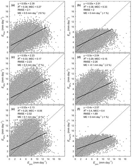
Figure 2.
Comparison between observations of daily total pan evaporation (EPan) (after applying the pan coefficient of 0.77) and models of potential evaporation based on: (a) Penman’s model (EPen); (b) the Priestley–Taylor model (EPT); (c) reference rate for grassland based on the Penman–Monteith model (d) reference rate for forests canopies that are moderately coupled to the atmosphere (ERFu); (e) reference rates for forest canopies that are well coupled to the atmosphere (ERFc); (f) linear mixed-effects model fit to daily pan evaporation measurements (EPanFit). Linear curves indicate the ordinary least squares fits. Statistics include: coefficient of determination (R2), model efficiency coefficient (MEC, values of 0.0 or <0.0 indicate equivalent, or less predictive power than applying the mean of observations, respectively, while a value of 1.0 indicates a perfect predictor), root mean squared error (RMSE, mm·day−1), and mean error (ME, mm·day−1 or %).
3.2. Monthly Model Comparison
Monthly variability of EPan ranged from 1.0 to 11.1 mm·day−1, with no major outliers (Figure 3). Of the individual meteorological drivers, the relationship was strongest between EPan and Rsgd and this relationship showed some indication of curvature (Figure 3a). Relationships with Ta and Da were weaker (Figure 3b,c), while there was no relationship between monthly EPan and U (Figure 3d).
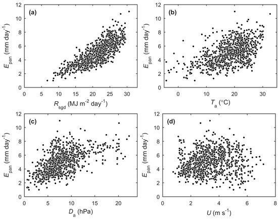
Figure 3.
Relationships between monthly mean pan evaporation (EPan) and climate variables, including incident global shortwave radiation (Rsgd), air temperature (Ta), vapour pressure deficit (Da), and wind speed (U).
Consistent with fits previously reported at the daily scale, all candidate predictor variables in the LME model fit to monthly EPan were significant (p < 0.001) (monthly LME model coefficients not shown). The marginal coefficient of determination for the monthly fit to pan evaporation was R2 = 0.68, with a mean (observation minus prediction) error of −0.16 ± 0.06 mm·day−1, and a root mean squared error of 0.93 mm·day−1.
Models listed in decreasing order of performance (i.e., agreement with monthly EPan measurements based on model efficiency coefficients), were EPanFit (MEC = 0.67), EPT (MEC = 0.64), EPen (MEC = 0.53), ERG (MEC = 0.31), ERFu (MEC = 0.10), and ERFc (MEC = −0.20) (Figure 4). The rate of evaporation for a reference forests with canopies that are moderately coupled to the atmosphere substantially underestimated EPan (Figure 4d). By design, these values were not expected to be unbiased expressions of PE, but we plotted them here to compare precision and explained variance for context. EPanFit slightly outperformed EPT, explaining 68% of the variance, with a mean error of −3% (Figure 4f). It is interesting to note that, despite slightly greater overall performance of EPanFit and EPT, these models still had limited capacity to reproduce the highest monthly values of EPan above 7.0 mm·day−1 (Figure 4b,f).
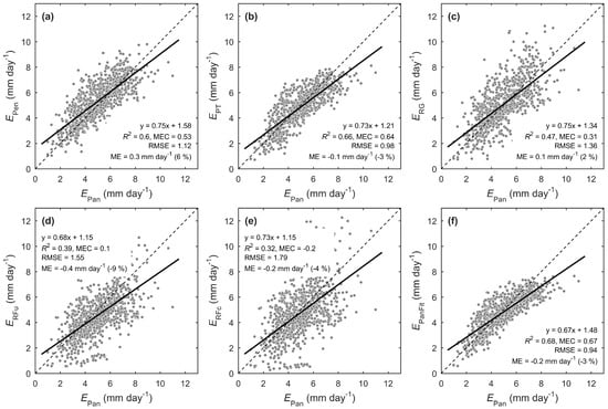
Figure 4.
Comparison between observations of monthly mean pan evaporation (EPan) and model predictions of potential evaporation (PE) based on: (a) Penman’s model; (b) the Priestley–Taylor model; (c) reference rates for grasslands based on the Penman–Monteith model; (d) reference rates for forests based on the Penman–Monteith model assuming the canopy is moderately coupled to the atmosphere; (e) reference rates for forests based on the Penman–Monteith model assuming the canopy is well coupled to the atmosphere; (f) linear mixed-effects model fit to monthly pan evaporation (EPanFit).
3.3. Attribution of Variance in PE to Meteorological Drivers
In decreasing order of sensitivity, daily variability of EPan was controlled by Rsgd, Ta, Da, and U (Figure 5). On a monthly time scale, the controls of Ta and Da on EPan dissipated and were compensated by increases in sensitivity to Rsgd, while control by U was no longer significant.

Figure 5.
The sensitivity of potential evaporation (PE) to driving variables on a daily and monthly time scale. Left-to-right (red bars): Fixed effects from linear mixed-effects model fits to daily pan evaporation (EPanFit); fixed effects from model fits to daily predictions of PE from Penman’s model; fixed effects from model fits to daily predictions of PE from the Priestley–Taylor model; fits to daily reference evaporation from grasslands based on the Penman–Monteith model; fits to daily reference evaporation from forest canopies that are moderately coupled to the atmosphere based on the Penman–Monteith model; fits to daily reference evaporation from forest canopies that are well coupled to the atmosphere based on the Penman–Monteith model. Blue bars then repeat through the same estimates, only for fits to monthly instead of daily time scale.
On a daily time scale, EPen was most strongly driven by Rsgd and secondarily by Da and U, while Ta exerted a low positive effect. There were no significant differences in sensitivity between daily and monthly time scale for EPen. EPT exhibited the strongest sensitivity to Rsgd, with secondary dependence on Ta. On a monthly time scale, control on EPT shifted slightly from Rsgd to Ta. Despite differences in aerodyne mic, the behaviour of ERFu and ERFc only showed modest differences in sensitivity to Da. Both exhibited strong dependence on Da, followed by Rsgd and weak positive dependence on Ta. Hence, none of the models perfectly matched the variance attribution of monthly EPanFit; sensitivity of monthly EPT to Ta was too high, while sensitivities of monthly EPen, ERFu, and ERFc to Da were too high.
3.4. Spatial and Temporal Variability
Differences in the spatial variation of PE were evident from visual inspection of the mean warm-season values over the 1971–2000 base period (Figure 6). Patterns for Penman’s model and the reference grassland PE were similar, with the exception that EPen showed slightly greater values of PE across regions of southern Canada (Figure 6a,c). The Priestley–Taylor model indicated relatively low PE in arid regions of the southwest U.S. compared to other models and also showed slightly greater levels of PE across southern Canada relative to ERG (Figure 6b). Reference forest values showed more prominent zonal gradients and the differences between spatial patterns of PE for moderately- and well-coupled canopies were much less than that between reference forest rates and other models (Figure 6d,e).
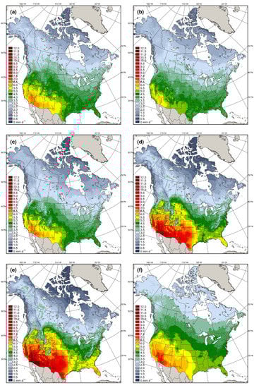
Figure 6.
Comparison between long-term (1971–2000) mean daily potential evaporation (PE) over the warm season (May–September). Units of PE are expressed as mm·day−1: (a) Penman’s model (EPen); (b) Priestley–Taylor model (EPT); (c) reference grassland (ERG) based on the Penman–Monteith model; (d) reference forest with moderately coupled canopy (ERFu) based on the Penman–Monteith model; (e) reference forest with coupled canopy (ERFc) based on the Penman–Monteith model; (f) linear mixed-effects model fit to monthly mean pan evaporation (EPanFit).
All models indicated decreases in warm-season mean daily PE as latitude increased from 25 to 80 degrees north (Figure 7). Zonal gradients were greatest for estimates of reference evaporation using the Penman–Monteith equation, and similar among other models. At the scale of ecozones, historical values of warm-season mean daily PE ranged from 2.4 to 4.5 mm·day−1 (Table 3). Mean historical values of warm-season PE ranged from 2.9 mm·day−1 (ERG) to 3.8 mm·day−1 (EPanFit) (Table 3).
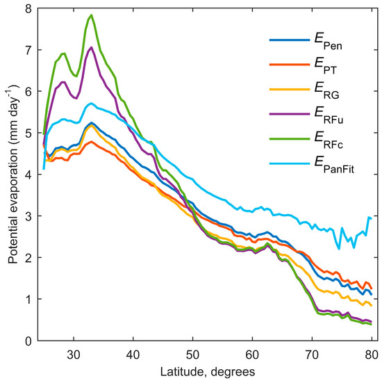
Figure 7.
Zonal mean warm-season (May–September) potential evaporation from various models over the land surface of North America.
Table 3.
Ecozone-average mean warm-season (May–September) variables over the period 1951–2014: Incident global solar radiation, Rsgd (MJ·m−2·day−1), air temperature, Ta (°C), vapour pressure, ea (hPa), vapour pressure deficit, Da (hPa), Penman’s model, EPen (mm·day−1), the Priestley–Taylor model, EPT (mm·day−1), the Penman–Monteith model for a reference grassland, ERG (mm·day−1), the Penman–Monteith model for a reference forest with moderately coupled canopy, ERFu (mm·day−1), and reference forest with well coupled canopy, ERFc (mm·day−1), and statistical fits to pan evaporation measurements EPanFit (mm·day−1).
On average over forest ecozones, there was little change in Rsgd from 1951–2014 (Table 4). According to NCEP/NCAR global reanalysis, Rsgd increased considerably over the boreal forest ecozones, and decreased considerably over eastern temperate forest ecozone. The station-based reconstruction of warm-season air temperature suggested an increase of 1.21 °C from 1951–2014 (Table 4). A large positive effect of warming on saturation vapour pressure led to a net increase in vapour pressure deficit of 0.81 hPa despite concomitant increase in vapour pressure of 0.38 hPa. No attempt was made to analyze trends in U.
Table 4.
Ecozone-average long-term changes in warm-season (May–September) mean daily variables over the period 1951–2014: Incident global solar radiation, Rsgd (MJ·m−2·day−1), air temperature, Ta (°C), vapour pressure deficit, Da (hPa), Penman’s model, EPen (mm·day−1), the Priestley–Taylor model, EPT (mm·day−1), the Penman–Monteith model for a reference grassland, ERG (mm·day−1), the Penman–Monteith model for a reference forest with moderately-coupled canopy, ERFu (mm·day−1), and reference forest with well-coupled canopy, ERFc (mm·day−1), and statistical fits to pan evaporation measurements EPanFit (mm·day−1).
Continuous high-resolution reconstructions of warm-season (May–September) mean PE based on values of EPen, EPT, ERG, ERFu, ERFc, and EPanFit suggested a range between negative and positive time trends from 1951–2014 (Figure 8). The magnitude of time trends were irregularly distributed, but similarities in the pattern were apparent among models. Negative trends were consistently concentrated over the east-central U.S. and pockets of industrialized areas across Canada and Alaska. On average across forest ecozones, the long-term change in estimates of potential evaporation (inferred from least-squares fits of potential evaporation against time for each model) ranged from just 0.08 mm·day−1 for the Priestley–Taylor model, to 0.45 mm·day−1 for the reference forest that is well coupled to the atmosphere (Table 4). Average long-term changes were intermediate for Penman’s model and the LME fit to pan evaporation measurements at 0.16 and 0.14 mm·day−1 respectively, slightly higher for the reference grassland (0.19 mm·day−1), and high for reference forests (0.37 and 0.45 mm·day−1 for moderately- and well-coupled canopies, respectively).
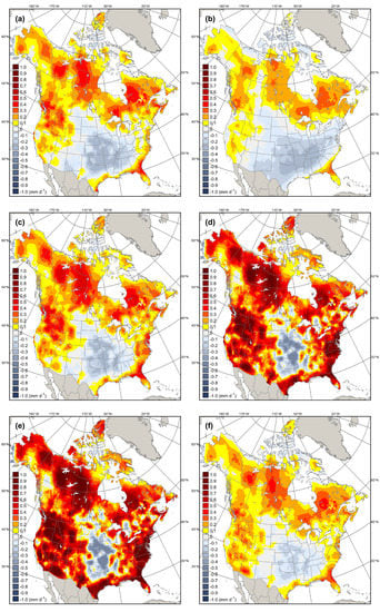
Figure 8.
Long-term change in warm-season (May–September) mean potential evaporation (PE) from 1951–2014 (mm·day−1): (a) Penman’s model (EPen); (b) Priestley–Taylor model (EPT); (c) reference grassland (ERG); (d) reference forest with moderately coupled canopy (ERFu); (e) reference forest with well coupled canopy (ERFc); (f) linear mixed-effects model fit to monthly mean pan evaporation (EPanFit). Values were calculated by multiplying the slope coefficient from regression relationship between PE and time by the length of the study period (64 years).
Based on a compilation of the time trends in warm-season PE for reference forests, using a range of aerodynamic and surface conductance, a general relationship was produced from regression analysis (Figure 9). The analysis confirmed that time trends increased strongly with increasing aerodynamic conductance and weakly with increasing surface conductance.

Figure 9.
Dependence of long-term changes in reference rates of evaporation on levels of aerodynamic conductance (ga) and surface conductance (gs) set in the Penman–Monteith equation. Trends are representative of mean warm-season daily reference evaporation over forest regions of North America (z-axis indicates change in mm·day−1 from 1951–2014).
4. Discussion
Ecological studies commonly make use of basic expressions of evaporative demand. Here, we explored the behavior of several common approaches to calculating PE. While such basic expressions of PE may have strong practical value in studies that attempt to predict climate change impacts on terrestrial ecosystems across large spatial and temporal domains, further work is needed to improve the representation of spatial variation in meteorological conditions above forests, canopy structure and physiology, and ultimately the prediction of actual evapotranspiration rather than PE or reference rates [52,53].
We considered measurements of pan evaporation as one independent indicator of PE. While there are likely key differences between PE above forests and evaporation pans, the comparison helped place the attribution of variance and spatial and temporal variability of PE predictions into context. Upon compiling the pan evaporation data from Canada and the U.S., we discovered that records were only rarely accompanied by on-site meteorological variables, so considerable effort was placed on deriving best available values from nearby climate stations, which constitutes an important source of error. Although varying conditions at the evaporation pans, and errors associated with site, wind, heating, splashing, likely led to different pan coefficients, we chose to restrict the scope of the study by applying a constant pan coefficient and including a random effect on the intercept coefficient at the scale of individual pan evaporation stations in the LME models. Applying a mid-range value of the pan coefficient, k = 0.77, led to a mean EPanFit of 3.8 mm·day−1 across North American forests. As this value was 0.5 mm·day−1 greater than the next highest value (EPen), any future consideration of the dataset should likely consider reducing k.
While plenty of surface water balance research is performed at a sub-monthly time interval, it remains far more practical to simulate the water balance at a monthly time step in large-scale forest ecosystem modelling. Analysis of variance attribution suggested that controls on EPan were scale dependent. On a daily time scale, EPan was significantly related to Rsgd, Ta, Da, and U, whereas on a monthly time scale EPan was only significantly related to Rsgd, Ta, and Da. We interpreted this difference to mean that systematic effects of advection (as an energy source over pans) and ground heat flux (as an energy sink) diminish as time scale increases. That is, on any given day, advection and ground heat flux can enhance or suppress PE, while beyond this temporal scale, it cancels out. The lack of effect of U at the monthly time scale may suggest that accuracy in large-scale analysis of spatial and temporal variation (including trend analysis) may not suffer from failure to represent wind.
Varying sensitivity to Da was a defining difference among the most popular models of PE. The Priestley–Taylor model and the Penman–Monteith model parameterized for conditions above reference forest canopies reflect estimates with absent Da-sensitivity and strong Da-sensitivity, respectively. Any inferences about change in surface hydrology and consequent socio-economic implications over time are, therefore, going to strongly depend on which model is applied. The differentiation in long-term change among models was exacerbated by strong apparent positive trend in historical Da across North America [85]. Interestingly, the different dependence on Da among models also shaped the zonal variation in PE (Figure 7), where estimates of PE derived from reference forest rates actually exceeded estimates of PE with infinite surface conductance in Penman’s model. Specifically, estimates of ERFu and ERFc start to exceed EPen when Da > 18.5 hPa.
On average across forests of North America, results indicate that PE increased from 1951–2014. If this is correct, increasing PE must increase the tendency for drought stress. Confidence in the claim of a positive trend is gained from the fact that all models consistently indicated positive trends. However, the claim of positive trends remains uncertain due to reliance on irradiance from NCEP/NCAR reanalysis, which has poorly constrained uncertainty, and by the inability to account for trends in wind speed. These sources of uncertainty will affect all models similarly. If we ignore uncertainty in irradiance and wind trends, it must still be recognized that the range of trend estimates among models of PE includes low estimates, which may have been exceeded by increasing trends in precipitation [86]. If we exclude consideration of EPT on the basis that it does not include dependence on Da, we estimate average long-term changes in warm season PE ranging from 0.14 to 0.45 mm·day−1. Hence, there is still large uncertainty in how much evaporative demand increased.
Greater increases in ERFu and ERFc, owing to strong dependence on increasing Da (and the general pattern of increasing trends with increasing ga and gs) must impose substantial impacts on the level of water stress imposed upon plants, either through a preemptive regulation of gas exchange to avoid desiccation at the expense of carbon supply, or lax regulation of gas exchange at the expense of water transport efficiency and risk of hydraulic failure. Yet either way, the magnitude of those increases in evaporative demand (i.e., the forcing imposed on guard cells or hydraulic conductivity) is not supported by other models of PE, including a statistical fit to EPan. That is not to say, however, that the more modest changes in evaporative demand implied by EPT cannot impose severe water stress, as the sensitivity of plant health and productivity to changes in EPT, specifically, remains largely unexplored.
At the regional scale, all trends in PE were positive with the exception of trends in the eastern temperate ecozone, where EPT was negative and EPen was zero. Interestingly, this could be the signature of high tropospheric aerosol forcing on surface climates over the east-central conterminous U.S. (Figure 8). Similar patterns exist for pockets of industrial activity across the continent. Further research is needed to understand the quantitative relationship between PE and tropospheric aerosols. If there is a link, it stands to reason that continued trends in PE may be strongly affected by the onset of aerosol emission regulations that began late in our study period (i.e., 1990’s), and conversely by any new or growing emission sources.
5. Conclusions
We investigated spatial and temporal variation of PE across forest regions of North America. While records of EPan were not long enough to perform direct trend analysis, we instead chose to produce a statistical model, EPanFit, that helped to place the magnitude of model predictions in context and evaluate differences in the relative effect of the driving meteorological factors. Consistent with previous model inter-comparison studies [1,87,88], we found substantial differences in PE among models. Large-scale (zonal) differences were clearly demonstrated across North America. Long-term change in PE from 1951–2014 ranged from 0.08 to 0.45 mm·day−1 depending on whether it was calculated with the Priestley–Taylor model, or with the Penman–Monteith model set for a reference forest by making the common assumption that the canopy is well coupled to the atmosphere. A general analysis of variance attribution among the approaches helped to put the underlying reasons for divergent behavior in quantitative terms. We conclude that until a consensus emerges on which expression is more representative of reality in forests, studies that adopt such basic expressions of PE should consider the range of different model predictions to represent uncertainty in trend magnitude. The need to forecast impacts of a changing climate forests, including wildfire risk, insect outbreak risk, drought-related mortality, and health decline syndromes, indicates a need to improve monitoring of the key drivers of PE, including Rsgd and Da. This source of high resolution, continuous monthly variation of PE from various models can facilitate research on a wide range of applications that require knowledge of the surface water balance.
Acknowledgments
This research was supported by the Pacific Institute for Climate Solutions.
Author Contributions
R.H., N.C., and D.S. designed the study. R.H. produced and analyzed results and wrote the first draft. R.H., N.C. and D.S. provided editorial comments and suggestions.
Conflicts of Interest
The authors declare no conflict of interest.
References
- Fisher, J.B.; Whittaker, R.J.; Malhi, Y. ET come home: Potential evapotranspiration in geographical ecology. Glob. Ecol. Biogeogr. 2011, 20, 1–18. [Google Scholar] [CrossRef]
- Webb, W.L.; Lauenroth, W.K.; Szarek, S.R.; Kinerson, R.S. Primary production and abiotic controls in forests, grasslands, and desert ecosystems in the united states. Ecology 1983, 64, 134–151. [Google Scholar] [CrossRef]
- Stephenson, N.L. Actual evapotranspiration and deficit: biologically meaningful correlates of vegetation distribution across spatial scales. J. Biogeogr. 1998, 25, 855–870. [Google Scholar] [CrossRef]
- Sperry, J.S.; Tyree, M.T. Water-stress-induced xylem embolism in three species of conifers. Plant Cell Environ. 1990, 13, 427–436. [Google Scholar] [CrossRef]
- Tyree, M.T.; Sperry, J.S. Do woody plants operate near the point of catastrophic xylem dysfunction caused by dynamic water stress? Answers from a model. Plant Physiol. 1988, 88, 574–580. [Google Scholar] [CrossRef] [PubMed]
- Choat, B.; Jansen, S.; Brodribb, T.J.; Cochard, H.; Delzon, S.; Bhaskar, R.; Bucci, S.J.; Feild, T.S.; Gleason, S.M.; Hacke, U.G.; et al. Global convergence in the vulnerability of forests to drought. Nature 2012, 491, 752–755. [Google Scholar] [CrossRef] [PubMed]
- Hember, R.A.; Kurz, W.A.; Coops, N.C. Relationships between individual-tree mortality and water-balance variables indicate positive trends in water stress-induced tree mortality across North America. Glob. Change Biol. 2016. [Google Scholar] [CrossRef] [PubMed]
- Millar, C.I.; Stephenson, N.L. Temperate forest health in an era of emerging megadisturbance. Science 2015, 349, 823–826. [Google Scholar] [CrossRef] [PubMed]
- McDowell, N.G.; Williams, A.P.; Xu, C.; Pockman, W.T.; Dickman, L.T.; Sevanto, S.; Pangle, R.; Limousin, J.; Plaut, J.; Mackay, D.S.; et al. Multi-scale predictions of massive conifer mortality due to chronic temperature rise. Nat. Clim. Change 2016, 6, 295–300. [Google Scholar] [CrossRef]
- Martínez-Vilalta, J.; Lloret, F. Drought-induced vegetation shifts in terrestrial ecosystems: The key role of regeneration dynamics. Glob. Planet. Change 2016, 144, 94–108. [Google Scholar] [CrossRef]
- Clark, J.S.; Iverson, L.; Woodall, C.W.; Allen, C.D.; Bell, D.M.; Bragg, D.C.; D’Amato, A.W.; Davis, F.W.; Hersh, M.H.; Ibanez, I.; et al. The impacts of increasing drought on forest dynamics, structure, and biodiversity in the United States. Glob. Change Biol. 2016. [Google Scholar] [CrossRef] [PubMed]
- Sucoff, E. Water potential in red pine: Soil moisture, evapotranspiration, crown position. Ecology 1972, 53, 681–686. [Google Scholar] [CrossRef]
- Sharkey, T.D. Transpiration-induced changes in the photosynthetic capacity of leaves. Planta 1984, 160, 143–150. [Google Scholar] [CrossRef] [PubMed]
- Novick, K.A.; Ficklin, D.L.; Stoy, P.C.; Williams, C.A.; Bohrer, G.; Oishi, A.C.; Papuga, S.A.; Blanken, P.D.; Noormets, A.; Sulman, B.N.; et al. The increasing importance of atmospheric demand for ecosystem water and carbon fluxes. Nat. Clim. Change 2016. [Google Scholar] [CrossRef]
- Sanderson, M. Drought in the Canadian Northwest. Geogr. Rev. 1948, 38, 289. [Google Scholar] [CrossRef]
- Thornthwaite, C.W. An approach toward a rational classification of climate. Geogr. Rev. 1948, 38, 55–94. [Google Scholar] [CrossRef]
- McMahon, T.A.; Peel, M.C.; Lowe, L.; Srikanthan, R.; McVicar, T.R. Estimating actual, potential, reference crop and pan evaporation using standard meteorological data: A pragmatic synthesis. Hydrol. Earth Syst. Sci. 2013, 17, 1331–1363. [Google Scholar] [CrossRef]
- Oke, T.R. Boundary Layer Climates, 2nd ed.; Routledge: Cambridge, UK, 1987. [Google Scholar]
- Rosenberg, N.; Blad, B.; Verma, S. Microclimate, the Biological Environment, 2nd ed.; Jon Wiley and Sons Inc.: Toronto, ON, Canada, 1983. [Google Scholar]
- Slatyer, R.; McIlroy, I. Practical Microclimatology. Commonw. Sci. Ind. Res. Organ. 1961. [Google Scholar] [CrossRef]
- Mather, J.R.; Ambroziak, R.A. A Search for Understanding Potential Evapotranspiration. Geogr. Rev. 1986, 76, 355–370. [Google Scholar] [CrossRef]
- Ferguson, H.L.; O’Neill, A.D.J.; Cork, H.F. Mean Evaporation over Canada. Water Resour. Res. 1970, 6, 1618–1633. [Google Scholar] [CrossRef]
- Kohler, M.A.; Nordenson, T.J.; Fox, W.E. Evaporation from Pans and Lakes; US Department of Commerce: Washington, DC, USA, 1955.
- Thornthwaite, C.W.; Mather, J.R. The Water Balance; Laboratory of Climatology: Centerton, NJ, USA, 1955. [Google Scholar]
- Hargreaves, G.H.; Allen, R.G. History and Evaluation of Hargreaves Evapotranspiration Equation. J. Irrig. Drain. Eng. 2003, 129, 53–63. [Google Scholar] [CrossRef]
- Christiansen, J.E. Estimating Evaporation and Evpoatranspiration from Climate Data; Utah Water Research Laboratory, Utah State University: Logan, UT, USA, 1966. [Google Scholar]
- Penman, H.L. Natural evaporation from open water, bare soil and grass. Proc. R. Soc. Lond. 1948, 193, 120–145. [Google Scholar] [CrossRef]
- Monteith, J.L. Evaporation and environment. Symp. Soc. Exp. Biol. 1965, 19, 205–234. [Google Scholar] [PubMed]
- Priestley, C.H.B.; Taylor, R.J. On the assessment of surface heat flux and evaporation using large-scale parameters. Mon. Weather Rev. 1972, 100, 81–92. [Google Scholar] [CrossRef]
- Black, T.A. Evapotranspiration from douglas-fir stands exposed to soil-water deficits. Water Resour. Res. 1979, 15, 164–170. [Google Scholar] [CrossRef]
- Brümmer, C.; Black, T.A.; Jassal, R.S.; Grant, N.J.; Spittlehouse, D.L.; Chen, B.; Nesic, Z.; Amiro, B.D.; Arain, M.A.; Barr, A.G.; et al. How climate and vegetation type influence evapotranspiration and water use efficiency in Canadian forest, peatland and grassland ecosystems. Agric. For. Meteorol. 2012, 153, 14–30. [Google Scholar] [CrossRef]
- Greve, P.; Seneviratne, S.I. Assessment of future changes in water availability and aridity. Geophys. Res. Lett. 2015, 42. [Google Scholar] [CrossRef] [PubMed]
- Hogg, E.H. Temporal scaling of moisture and the forest-grassland boundary in western Canada. Agric. For. Meteorol. 1997, 84, 115–122. [Google Scholar] [CrossRef]
- Willmott, C.J.; Rowe, C.M.; Mintz, Y. Climatology of the terrestrial seasonal water cycle. J. Climatol. 1985, 5, 589–606. [Google Scholar] [CrossRef]
- Allen, R.G.; Pereira, L.S.; Raes, D.; Smith, M. Crop Evapotranspiration: Guidelines for Computing Crop Water Requirements, FAO Irrigation and Drainage Paper 56; Food and Agriculture Organization of the United Nations: Rome, Italy, 1998. [Google Scholar]
- Cleugh, H.A.; Leuning, R.; Mu, Q.Z.; Running, S.W. Regional evaporation estimates from flux tower and MODIS satellite data. Remote Sens. Environ. 2007, 106, 285–304. [Google Scholar] [CrossRef]
- Spittlehouse, D.L. Water availability, climate change and the growth of Douglas-fir in the Georgia Basin. Can. Water Resour. J. 2003, 28, 673–687. [Google Scholar] [CrossRef]
- Coops, N.; Coggins, S.; Kurz, W. Mapping the environmental limitations to growth of coastal Douglas-fir stands on Vancouver Island, British Columbia. Tree Physiol. 2007, 27, 805–815. [Google Scholar] [CrossRef] [PubMed]
- Seely, B.; Welham, C.; Scoullar, K. Application of a hybrid forest growth model to evaluate climate change impacts on productivity, nutrient cycling and mortality in a montane forest ecosystem. PLoS ONE 2015, 10, e0135034. [Google Scholar] [CrossRef] [PubMed]
- King, D.A.; Bachelet, D.M.; Symstad, A.J.; Ferschweiler, K.; Hobbins, M. Estimation of potential evapotranspiration from extraterrestrial radiation, air temperature and humidity to assess future climate change effects on the vegetation of the Northern Great Plains, USA. Ecol. Model. 2015, 297, 86–97. [Google Scholar] [CrossRef]
- Hogg, E.H.; Barr, A.G.; Black, T.A. A simple soil moisture index for representing multi-year drought impacts on aspen productivity in the western Canadian interior. Agric. For. Meteorol. 2013, 178–179, 173–182. [Google Scholar] [CrossRef]
- Wang, Y.; Hogg, E.H.; Price, D.T.; Edwards, J.; Williamson, T. Past and projected future changes in moisture conditions in the Canadian boreal forest. For. Chron. 2014, 90, 678–691. [Google Scholar] [CrossRef]
- Chattopadhyay, N.; Hulme, M. Evaporation and potential evapotranspiration in India under conditions of recent and future climate change. Agric. For. Meteorol. 1997, 87, 55–73. [Google Scholar] [CrossRef]
- Hobbins, M.; Ramirez, J.; Brown, T. Trends in pan evaporation and actual evapotranspiration across the conterminous US: Paradoxical or complementary? Geophys. Res. Lett. 2004, 31. [Google Scholar] [CrossRef]
- Linacre, E.T. Estimating U.S. Class A pan evaporation from few climate data. Water Int. 1994, 19, 5–14. [Google Scholar] [CrossRef]
- Hobbins, M.T.; Dai, A.; Roderick, M.L.; Farquhar, G.D. Revisiting the parameterization of potential evaporation as a driver of long-term water balance trends. Geophys. Res. Lett. 2008, 35, L12403. [Google Scholar] [CrossRef]
- Kingston, D.G.; Todd, M.C.; Taylor, R.G.; Thompson, J.R.; Arnell, N.W. Uncertainty in the estimation of potential evapotranspiration under climate change. Geophys. Res. Lett. 2009, 36, L20403. [Google Scholar] [CrossRef]
- Scheff, J.; Frierson, D.M.W. Scaling potential evapotranspiration with greenhouse warming. J. Clim. 2013, 27, 1539–1558. [Google Scholar] [CrossRef]
- Dai, A. Increasing drought under global warming in observations and models. Nat. Clim. Change 2013, 3, 52–58. [Google Scholar] [CrossRef]
- Dai, A. Characteristics and trends in various forms of the Palmer Drought Severity Index during 1900–2008. J. Geophys. Res. Atmospheres 2011, 116. [Google Scholar] [CrossRef]
- Sheffield, J.; Wood, E.F.; Roderick, M.L. Little change in global drought over the past 60 years. Nature 2012, 491, 435–438. [Google Scholar] [CrossRef] [PubMed]
- Amatya, D.; Tian, S.; Dai, Z.; Sun, G. Long-term potential and actual evapotranspiration of two different forests on the Atlantic Coastal Plain. Trans. ASABE 2016, 59, 647–660. [Google Scholar]
- Brauman, K.A.; Freyberg, D.L.; Daily, G.C. Potential evapotranspiration from forest and pasture in the tropics: A case study in Kona, Hawai‘i. J. Hydrol. 2012, 440–441, 52–61. [Google Scholar] [CrossRef]
- NREL 2013 US Department of Energy, National Renewable Energy Laboratory. National Solar Radiation Data Base. Available online: http://rredc.nrel.gov/solar/old_data/nsrdb/ (accessed on 26 April 2016).
- GSOD 2013 National Oceanic and Atmospheric Administration, Global Summary of the Day. Available online: https://data.noaa.gov/dataset/global-surface-summary-of-the-day-gsod (accessed on 31 October 2013).
- Brouwer, C.; Heibloem, M. Irrigation Water Management: Irrigation Water Needs; Food and Agriculture Orgainzation of the United Nations: Rome, Italy, 1985. [Google Scholar]
- Lu, J.; Sun, G.; McNulty, S.G.; Amatya, D. A comparison of six potential evapotranspiration methods for regional use in the Southeastern United States. J. Am. Water Resour. Assoc. 2005, 41, 621–633. [Google Scholar] [CrossRef]
- Kelliher, F.; Leuning, R.; Schulze, E. Evaporation and canopy characteristics of coniferous forests and grasslands. Oecologia 1993, 95, 153–163. [Google Scholar] [CrossRef]
- Landsberg, J.; Sands, P. Physiological Ecology of Forest Production: Principles, Processes and Models, 1st ed.; Elsevier Inc.: Boston, MA, USA, 2011. [Google Scholar]
- Pereira, A.R. The Priestley–Taylor parameter and the decoupling factor for estimating reference evapotranspiration. Agric. For. Meteorol. 2004, 125, 305–313. [Google Scholar] [CrossRef]
- Bladon, K.D.; Silins, U.; Landhäusser, S.M.; Lieffers, V.J. Differential transpiration by three boreal tree species in response to increased evaporative demand after variable retention harvesting. Agric. For. Meteorol. 2006, 138, 104–119. [Google Scholar] [CrossRef]
- Humphreys, E.; Black, T.; Ethier, G.; Drewitt, G.; Spittlehouse, D.; Jork, E.; Nesic, Z.; Livingston, N. Annual and seasonal variability of sensible and latent heat fluxes above a coastal Douglas-fir forest, British Columbia, Canada. Agric. For. Meteorol. 2003, 115, 109–125. [Google Scholar] [CrossRef]
- Martin, T.A.; Hinckley, T.M.; Meinzer, F.C.; Sprugel, D.G. Boundary layer conductance, leaf temperature and transpiration of Abies amabilis branches. Tree Physiol. 1999, 19, 435–443. [Google Scholar] [CrossRef] [PubMed]
- Jarvis, P.G.; McNaughton, K.G. Stomatal Control of Transpiration: Scaling Up from Leaf to Region. In Advances in Ecological Research; Elsevier: Amsterdam, The Netherlands, 1986; Volume 15, pp. 1–49. [Google Scholar]
- Running, S.; Coughlan, J. A General-Model of Forest Ecosystem Processes for Regional Applications. 1. Hydrologic Balance, Canopy Gas-Exchange and Primary Production Processes. Ecol. Model. 1988, 42, 125–154. [Google Scholar] [CrossRef]
- Bates, D.M. Lme4: Mixed-Effects Modeling with R; Springer: New York, NY, USA, 2010. [Google Scholar]
- Kalnay, E.; Kanamitsu, M.; Kistler, R.; Collins, W.; Deaven, D.; Gandin, L.; Iredell, M.; Saha, S.; White, G.; Woollen, J.; et al. The NCEP/NCAR 40-year reanalysis project. Bull. Am. Meteorol. Soc. 1996, 77, 437–471. [Google Scholar] [CrossRef]
- Schroeder, T.; Hember, R.; Coops, N.; Liang, S. Validation of solar radiation surfaces from modis and reanalysis data over topographically complex terrain. J. Appl. Meteorol. Climatol. 2009, 48, 2441–2458. [Google Scholar] [CrossRef]
- NARR 2013 National Oceanic and Atmospheric Administration, Earth System Research Laboratory. North American Regional Reanalysis. Available online: www.esrl.noaa.gov/psd/data/gridded (accessed on 18 December 2013).
- ESRI. ArcGIS 2013 ArcGIS 9.2 Desktop Help. Available online: webhelp.esri.com/arcgisdesktop/9.2/index.cfm?TopicName=Area_Solar_Radiation (accessed on 23 July 2013).
- Cogley, J.G. Greenland accumulation: An error model. J. Geophys. Res. Atmospheres 2004, 109. [Google Scholar] [CrossRef]
- Press, W.; Teukolsky, S.; Vetterling, W.; Flannery, B. Numerical Recipes: The Art of Scientific Computing, 3rd ed.; Cambridge Universiy Press: New York, NY, USA, 2007. [Google Scholar]
- Wang, T.; Hamann, A.; Spittlehouse, D.; Aitken, S. Development of scale-free climate data for western Canada for use in resource management. Int. J. Climatol. 2006, 26, 383–397. [Google Scholar] [CrossRef]
- Wang, T.; Hamann, A.; Spittlehouse, D.; Carroll, C. Locally downscaled and spatially customizable climate data for historical and future periods for north america. PLoS ONE 2016, 11, e0156720. [Google Scholar] [CrossRef] [PubMed]
- EC-NCDIA 2013 Environment Canada, National Climate Data and Information Archive. 2013. Available online: http://climate.weather.gc.ca/index_e.html (accessed on 5 January 2013).
- Menne, M.J.; Williams, C.N.; Vose, R.S. United States Historical Climatology Network (USHCN); Version 2.5 Serial Monthly Dataset; Oak Ridge National Laboratory, Carbon Dioxide Information Analysis Center: Oak Ridge, TN, USA.
- EC-AHCCD 2013 Environment Canada, Adjusted and Homogenized Canadian Climate Data. 2013. Available online: http://www.ec.gc.ca/dccha-ahccd/ (accessed on 15 July 2013).
- CRU31 2013 UK Met Office, Climate Research Unit. Climate Database, Version 3.1; Available online: http://badc.nerc.ac.uk/view/badc.nerc.ac.uk__ATOM__dataent_1256223773328276 (accessed on 25 July 2013).
- Kimball, J.; Running, S.; Nemani, R. An improved method for estimating surface humidity from daily minimum temperature. Agric. For. Meteorol. 1997, 85, 87–98. [Google Scholar] [CrossRef]
- Thornton, P.; Running, S.; White, M. Generating surfaces of daily meteorological variables over large regions of complex terrain. J. Hydrol. 1997, 190, 214–251. [Google Scholar] [CrossRef]
- USGS National Atlas of the United States. Available online: https://nationalmap.gov/small_scale/ (accessed on 13 March 2015).
- Coakley, J.A. Reflectance and albedo, surface. In Encyclopedia of the Atmospheric Sciences; Holton, J.R., Curry, J.A., Pyle, J.A., Eds.; Academic Press: Cambridge, MA, USA, 2002; pp. 1914–1923. [Google Scholar]
- Oak Ridge National Laboratory Distributed Active Archive Center (ORNL DAAC). FLUXNET Web Page; ORNL DAAC: Oak Ridge, TN, USA, 2015. [Google Scholar]
- CEC 1997 Commission for Environmental Cooperation (CEC): Ecological Regions of North America—Towards a Common Perspective. GIS Data (shapefiles, metadata and symbology). Available online: http://www.cec.org/tools-and-resources/map-files/terrestrial-ecoregions-level-i (accessed on 29 November 2009).
- Isaac, V.; van Wijngaarden, W.A. Surface water vapor pressure and temperature trends in North America during 1948–2010. J. Clim. 2012, 25, 3599–3609. [Google Scholar] [CrossRef]
- Vincent, L.A.; Zhang, X.; Brown, R.D.; Feng, Y.; Mekis, E.; Milewska, E.J.; Wan, H.; Wang, X.L. Observed Trends in Canada’s Climate and Influence of Low-Frequency Variability Modes. J. Clim. 2015, 28, 4545–4560. [Google Scholar] [CrossRef]
- Vörösmarty, C.J.; Federer, C.A.; Schloss, A.L. Potential evaporation functions compared on US watersheds: Possible implications for global-scale water balance and terrestrial ecosystem modeling. J. Hydrol. 1998, 207, 147–169. [Google Scholar] [CrossRef]
- Yao, H. Long-term study of lake evaporation and evaluation of seven estimation methods: Results from Dickie Lake, south-central Ontario, Canada. J. Water Resour. Prot. 2009, 1, 59–77. [Google Scholar] [CrossRef]
© 2017 by the authors; licensee MDPI, Basel, Switzerland. This article is an open access article distributed under the terms and conditions of the Creative Commons Attribution (CC-BY) license (http://creativecommons.org/licenses/by/4.0/).