
Provision of Desalinated Irrigation Water by the Desalination of Groundwater within a Saline Aquifer

Abstract
:1. Introduction
1.1. Impact of Irrigation Water Salinity on Crop Yield
- (i)
- Is the technology likely to produce an adequate amount of water for a reasonable cost over a reasonable timeframe?
- (ii)
- Is the application, by irrigation, of the desalinated (or partially desalinated) water, likely to make a significant impact on the revenue and profitability of the agricultural holding?
1.2. Maximum Sustainable Desalination Cost for Saline Irrigation Water
1.3. Zero Valent Iron
- (a)
- (b)
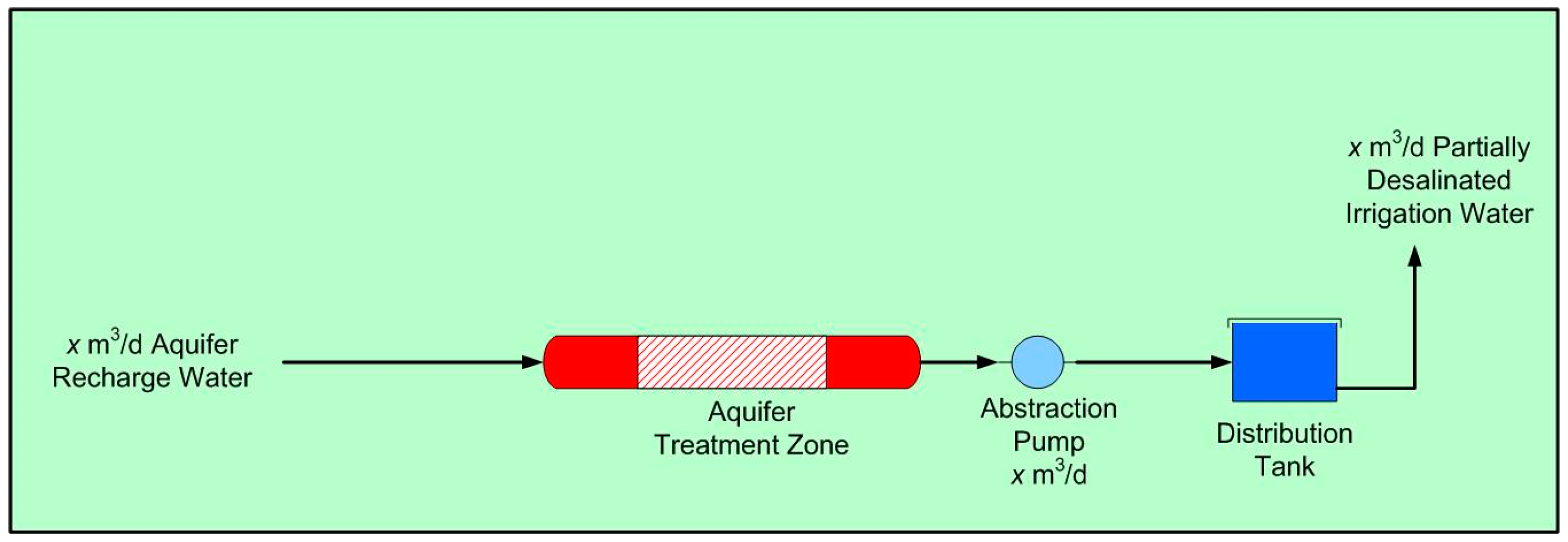
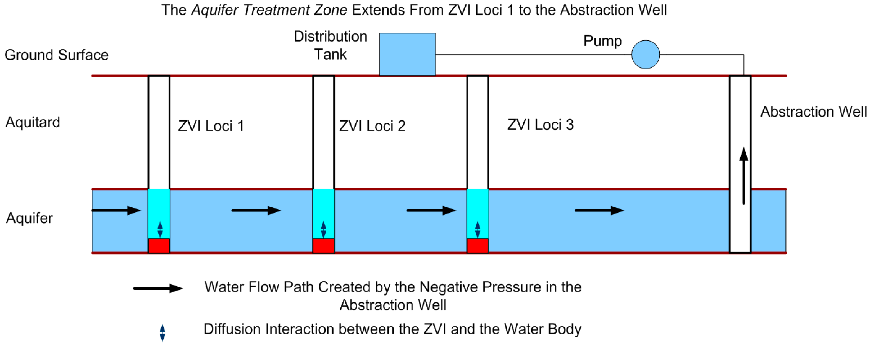
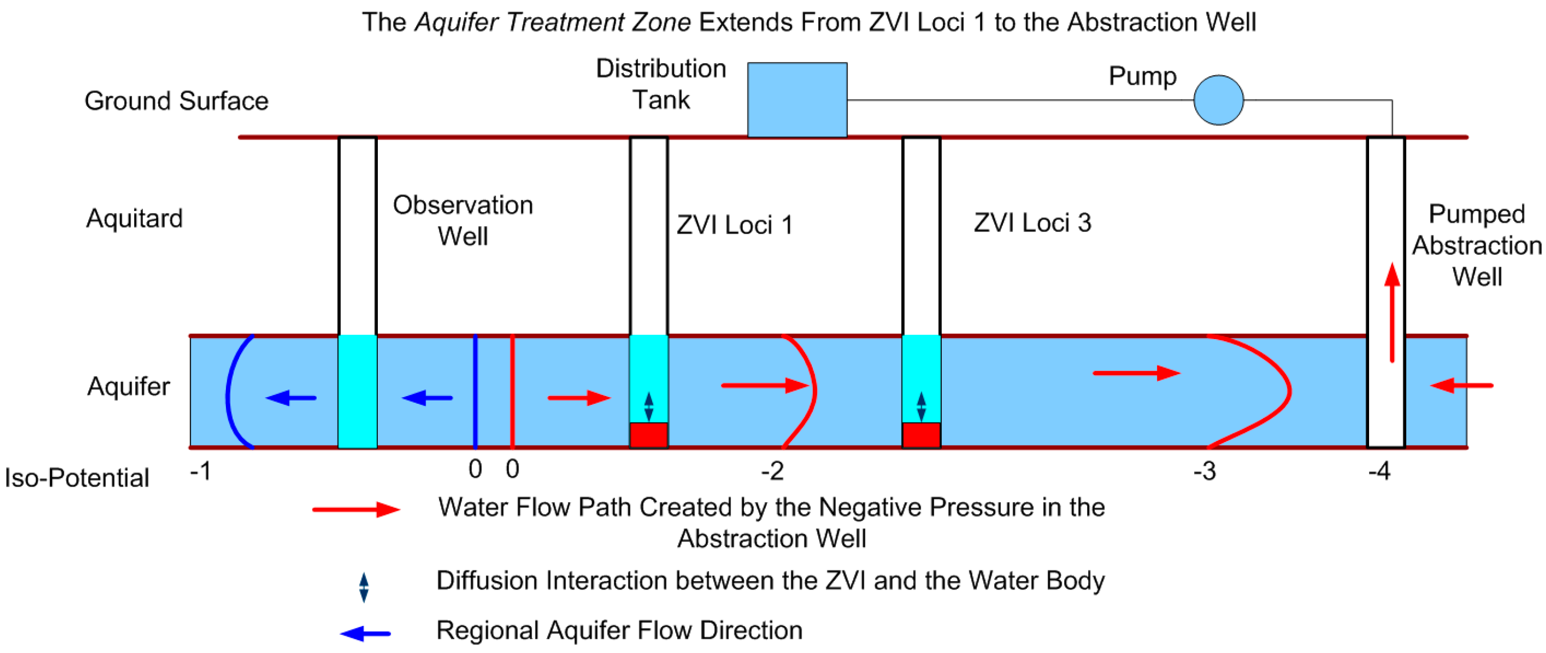
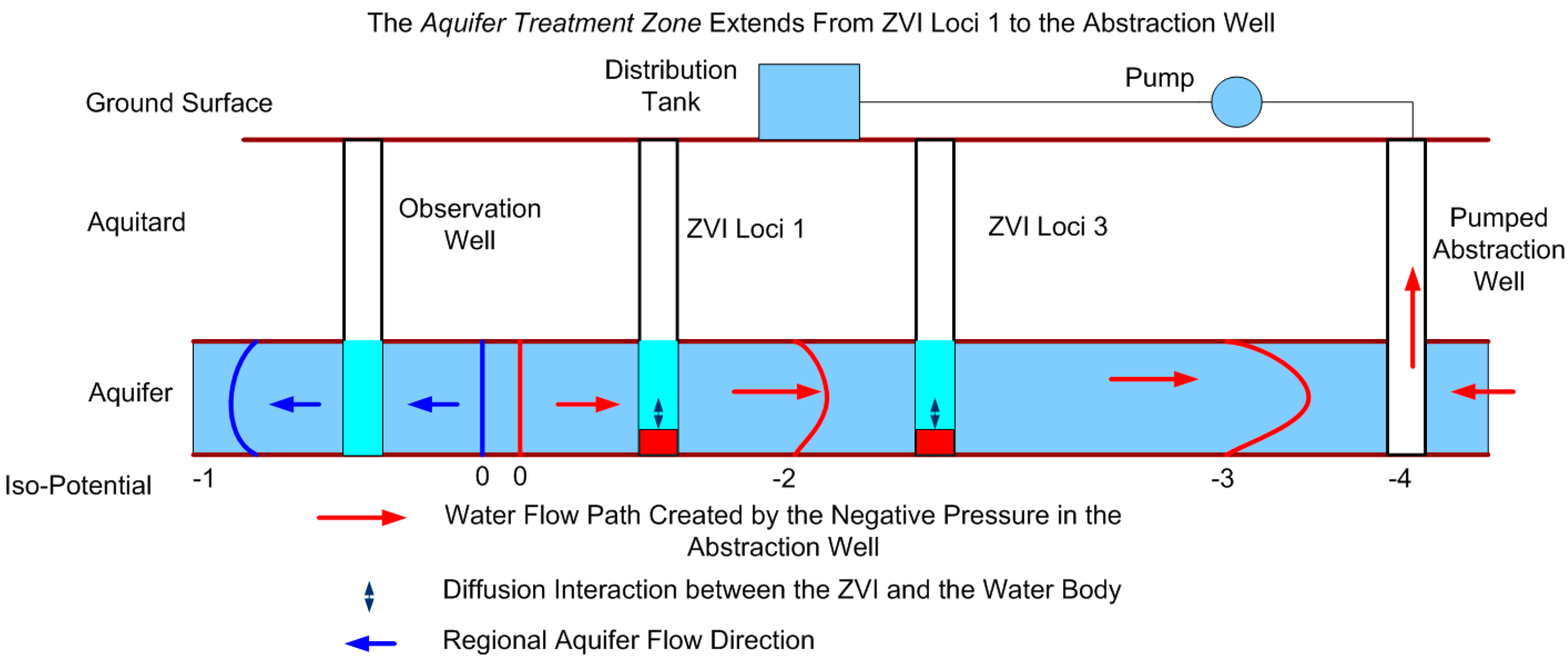
1.4. Definition and Construction of an Aquifer Treatment Zone
- Appendix B: Kinetic Data associated ST series desalination pellets; Equation (B1); Figure B1, Figure B2 and Figure B3;
- Appendix D: Classifying the Potential Aquifer Resource;
- Appendix E: Calculating and modeling the dimensions associated with a proposed Aquifer Treatment Zone. Equations (E1)–(E5); Table E1;
- Appendix G: Modeling a potential Static Strategy when the Aquifer is heterogenous; Equations (G1)–(G4); Figure G1.
2. Desalination Product
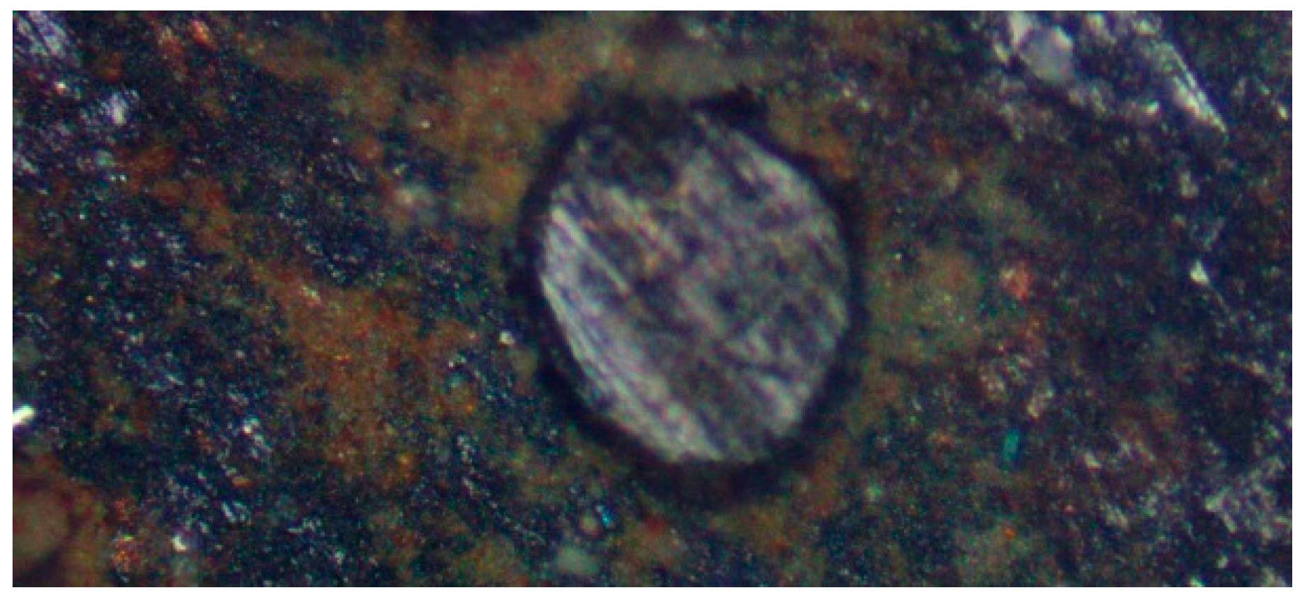
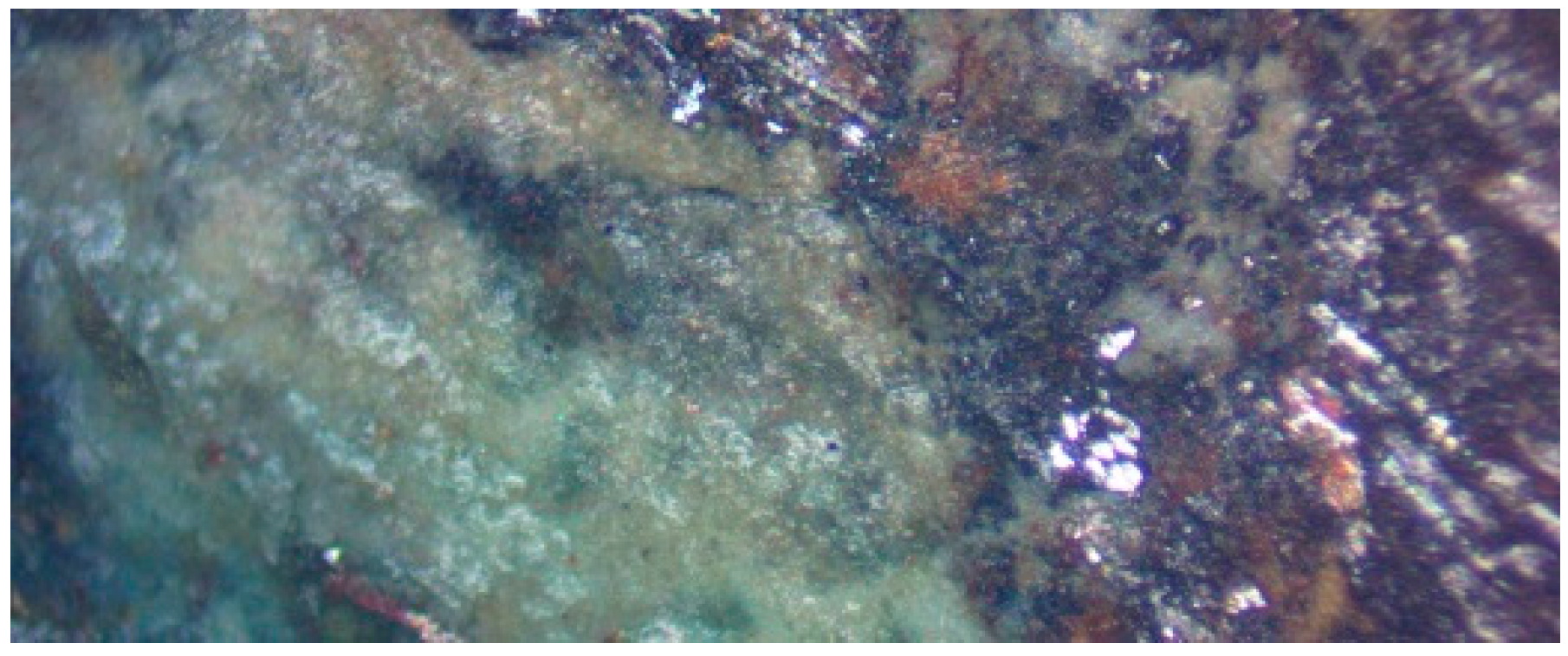
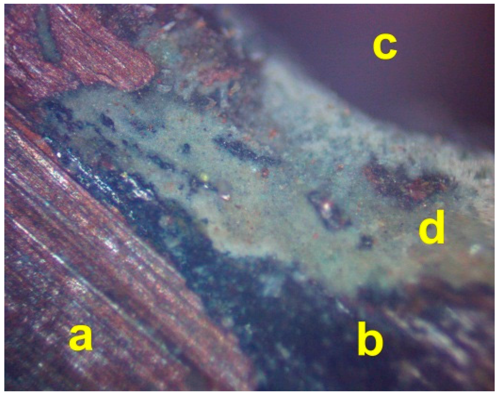
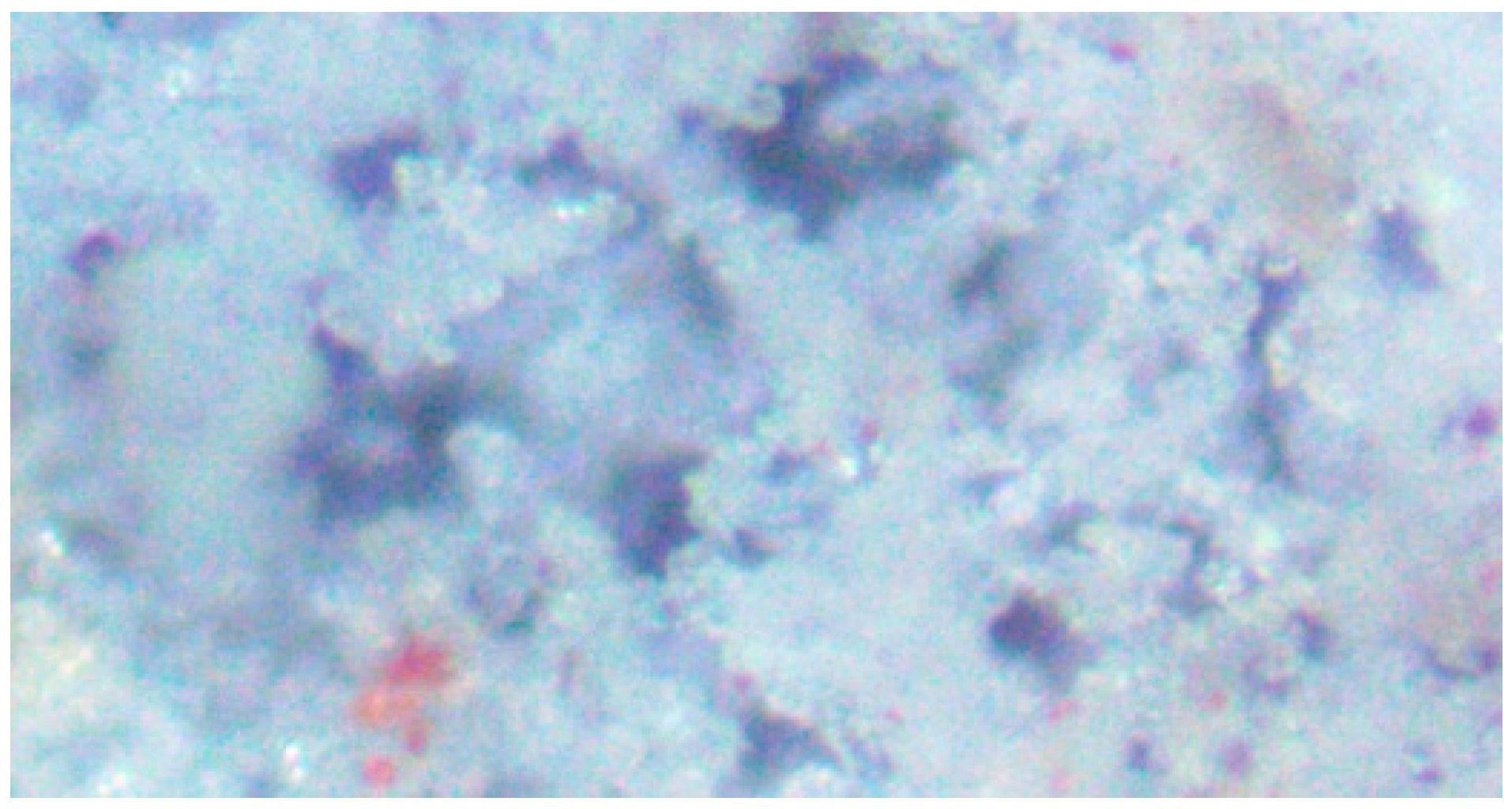
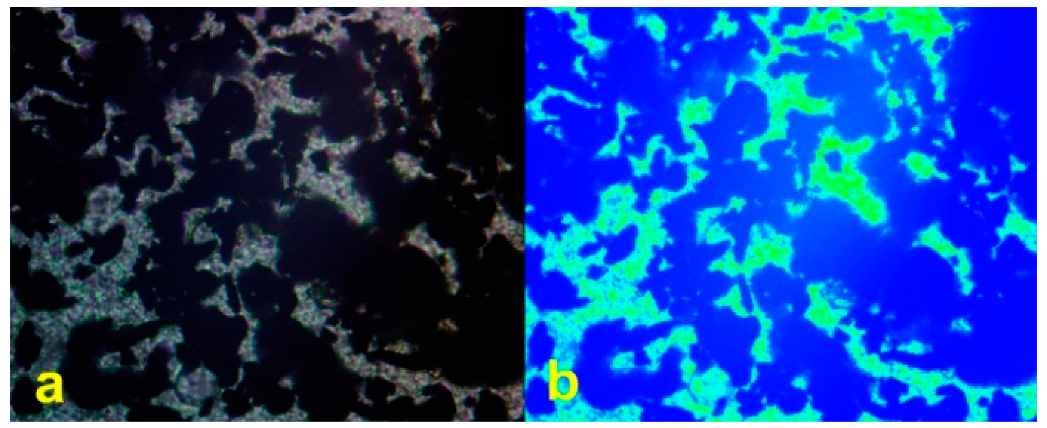
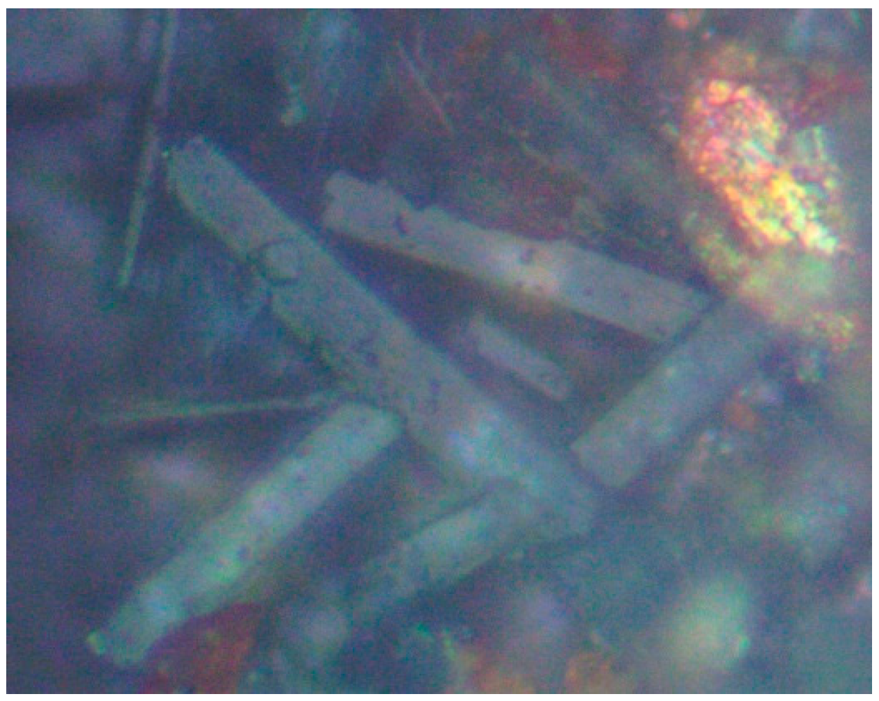
3. Desalination Product Petrography
3.1. Hygroscopic Nature of Cut Pellets
3.2. Rough Surface of Cut Pellets Following Desalination
3.3. Polished Surface of Cut Pellets Following Desalination
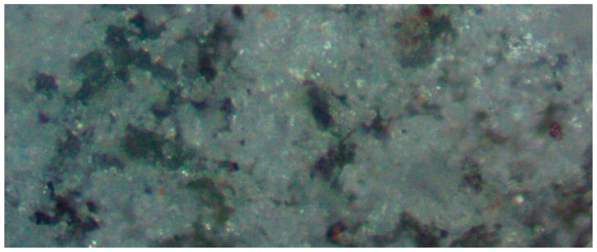
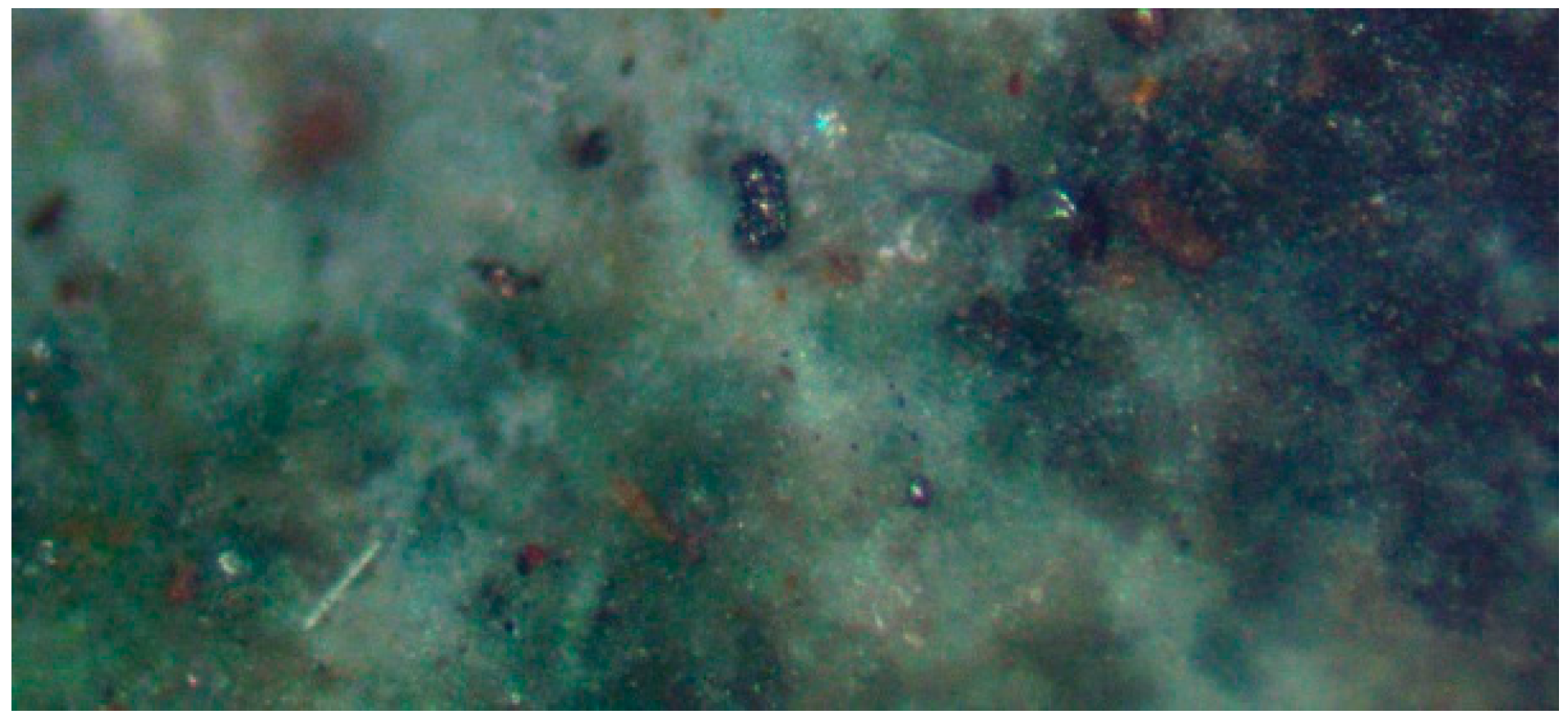
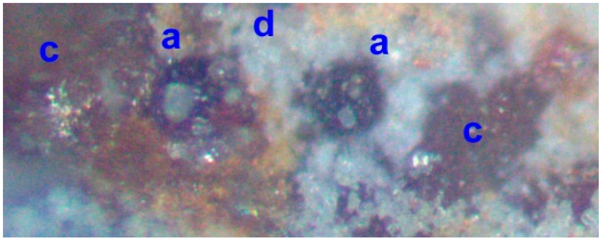
3.4. Material Redistribution within the Pellets during Desalination
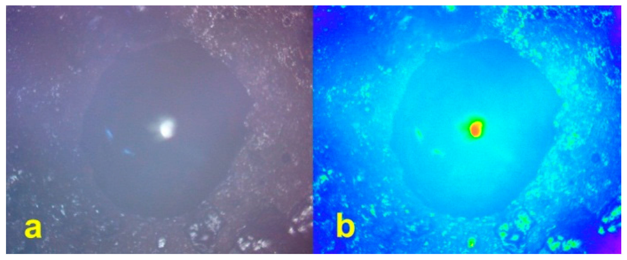
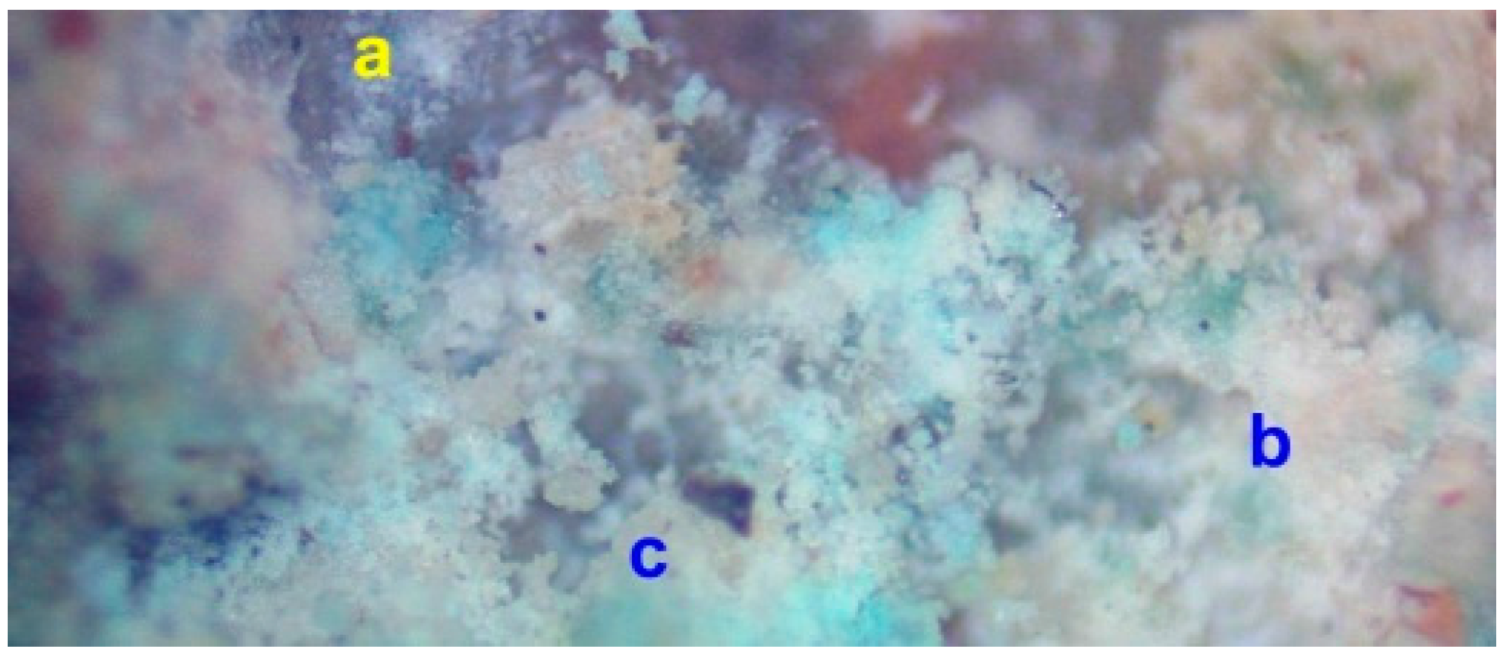
3.5. Reprecipitation of Copper within the Pellets during Desalination
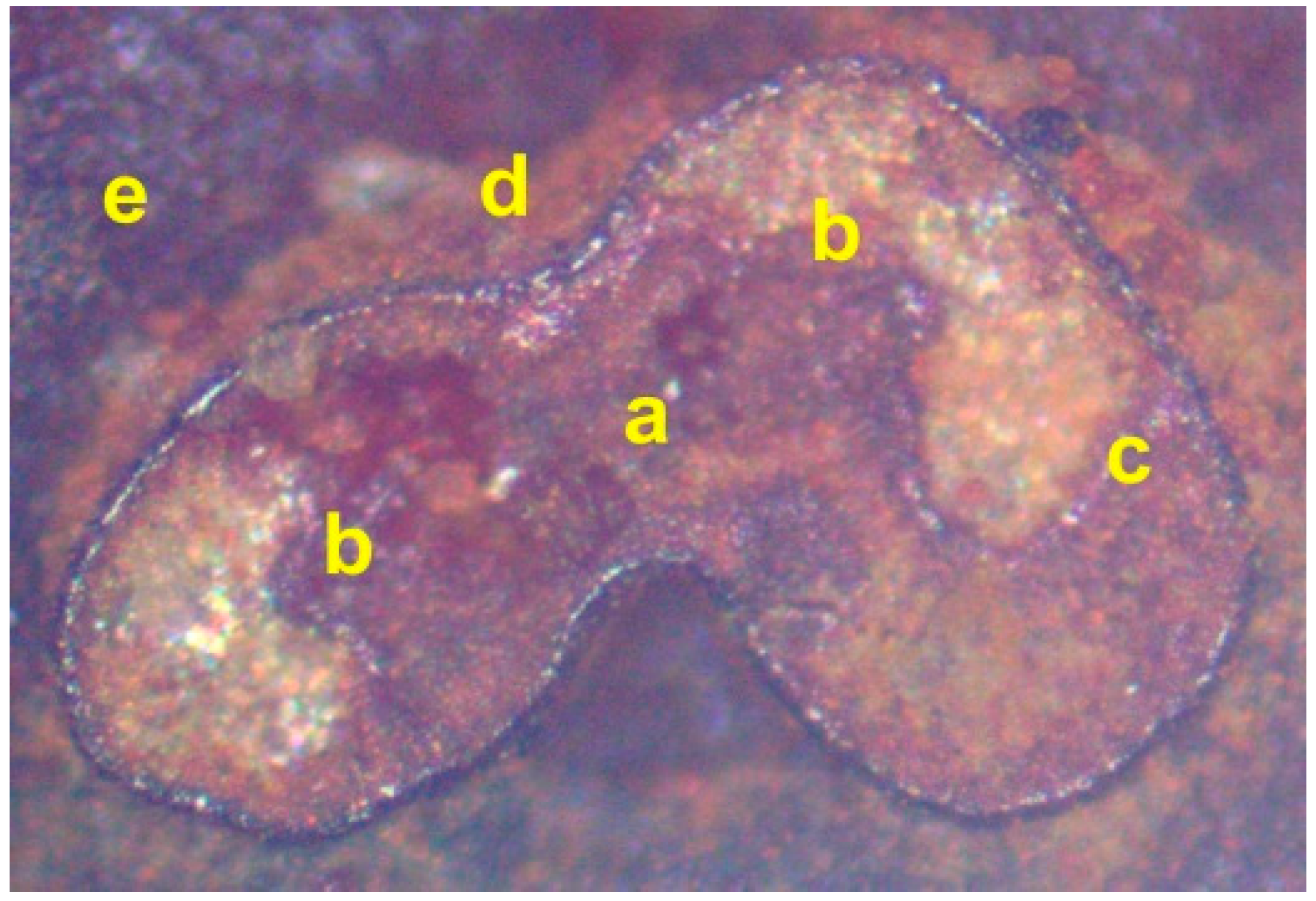
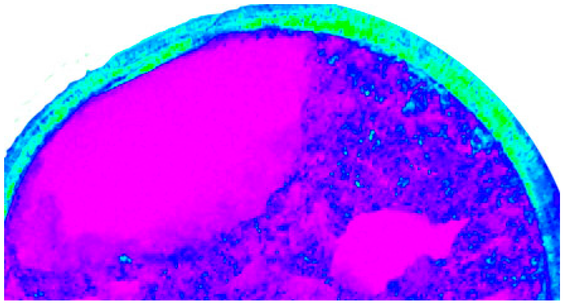
3.6. Method of Halite Infill of Porosity within the Pellets during Desalination
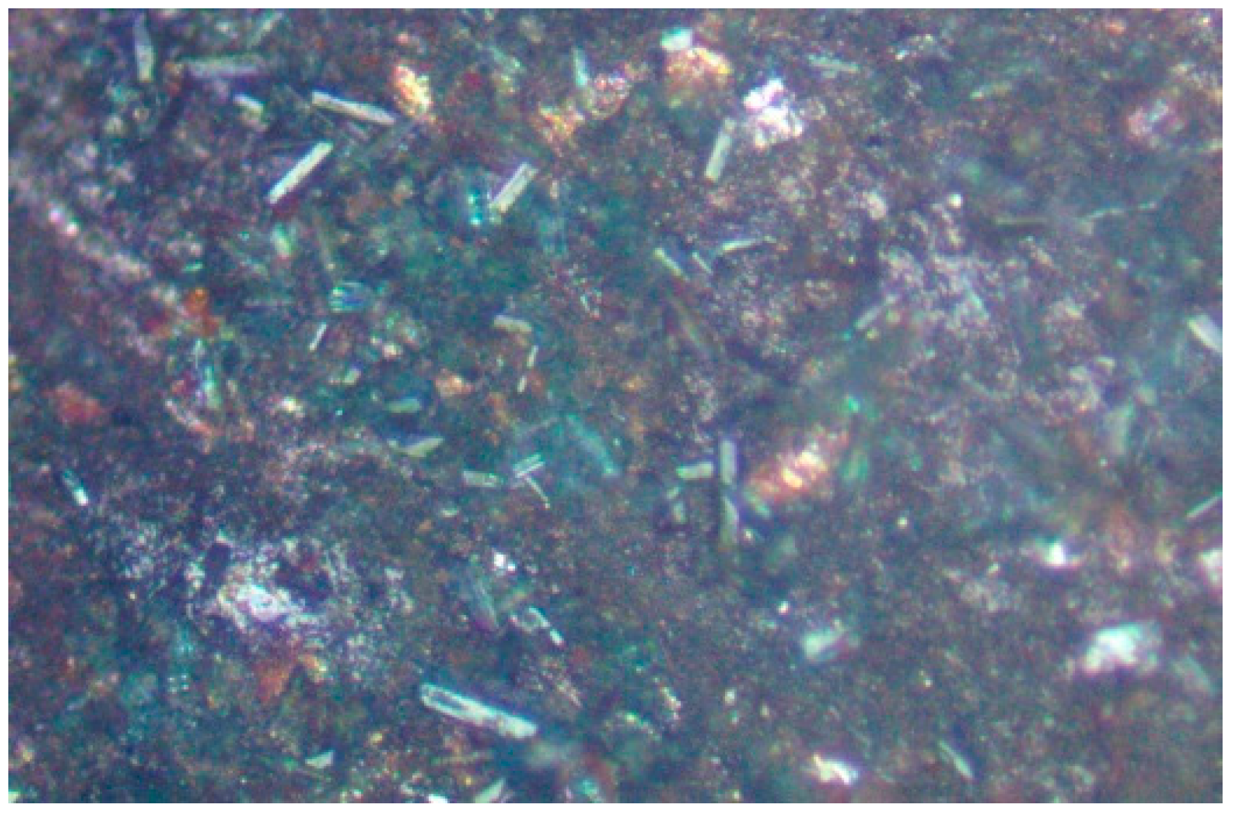
3.7. Morphology of Halite Infill of Porosity within the Pellets during Desalination
3.8. Morphology of Halite Infill of Porosity
3.9. Ironstone Precipitation
4. Chemical Implications of the Petrography for Aquifer Desalination
4.1. Dubinin-Astakhov Catalytic Model for ZVI Desalination
4.2. Significance of Porosity within the ZVI
- (a)
- (b)
- Placement of desorbed Na+ and Cl− ions into pores (Vop) which are in direct communication with the main water body will result in the desorbed Na+ and Cl− ions returning to the main water body. Vop > 0% at t = 0;
- (c)
- The inter-particle porosity = ϕ = Vo + Vop, and Vo = a·ϕ; Vop = b·ϕ, where a + b = 1. Once Vx/Vo = 1, {a} = 0, the residual porosity is Vop, i.e., {b} = 1. An irreducible water salinity level, BS, occurs when {a} reduces to 0.
4.3. Significance of Fluid Pore Pressure within the ZVI Pellet
- Na+ and Cl− ion removal rates will increase with increased pressure differentials between the pressures in the pores and the wider aquifer;
- Na+ and Cl− removal can have different rate constants [17];
- Smaller pores will be filled preferentially relative to larger pores.
5. Catalytic Implications of the Petrography
Desalination Model
6. Commercial Implications of the Petrography for Aquifer Desalination
7. Hydrological and Chemical Engineering Requirements for Commercialization
7.1. Conceptual and Front-End Hydrological Engineering and Design (FEHED)
- (a)
- 15 mm diameter Cu0 cased pellets (without operational optimization) = 59.1% to 65.8%, n = 50;
- (b)
- 75 mm diameter MDPI cased pellets (without operational optimization) = 58.2% to 83.4%, n = 15. i.e., 99% confidence limits (BS2846) are: mean ± (Standard Deviation) (t0.995/(n)0.5), where n = number of samples; t0.995 is the value (for n) of the students t test distribution (at the 99% confidence limits).
- prospective resource;
- contingent resource;
- developed resource.
7.2. Scale Up of Trial Desalination Kinetic Data to Provide an Assessment of the Amount of ZVI Required and the Size of the Aquifer Treatment Zone
- Up scaling the ZVI quantities used in the trials:
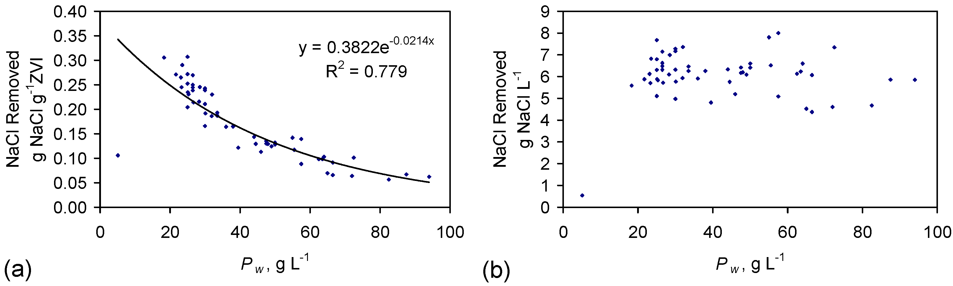
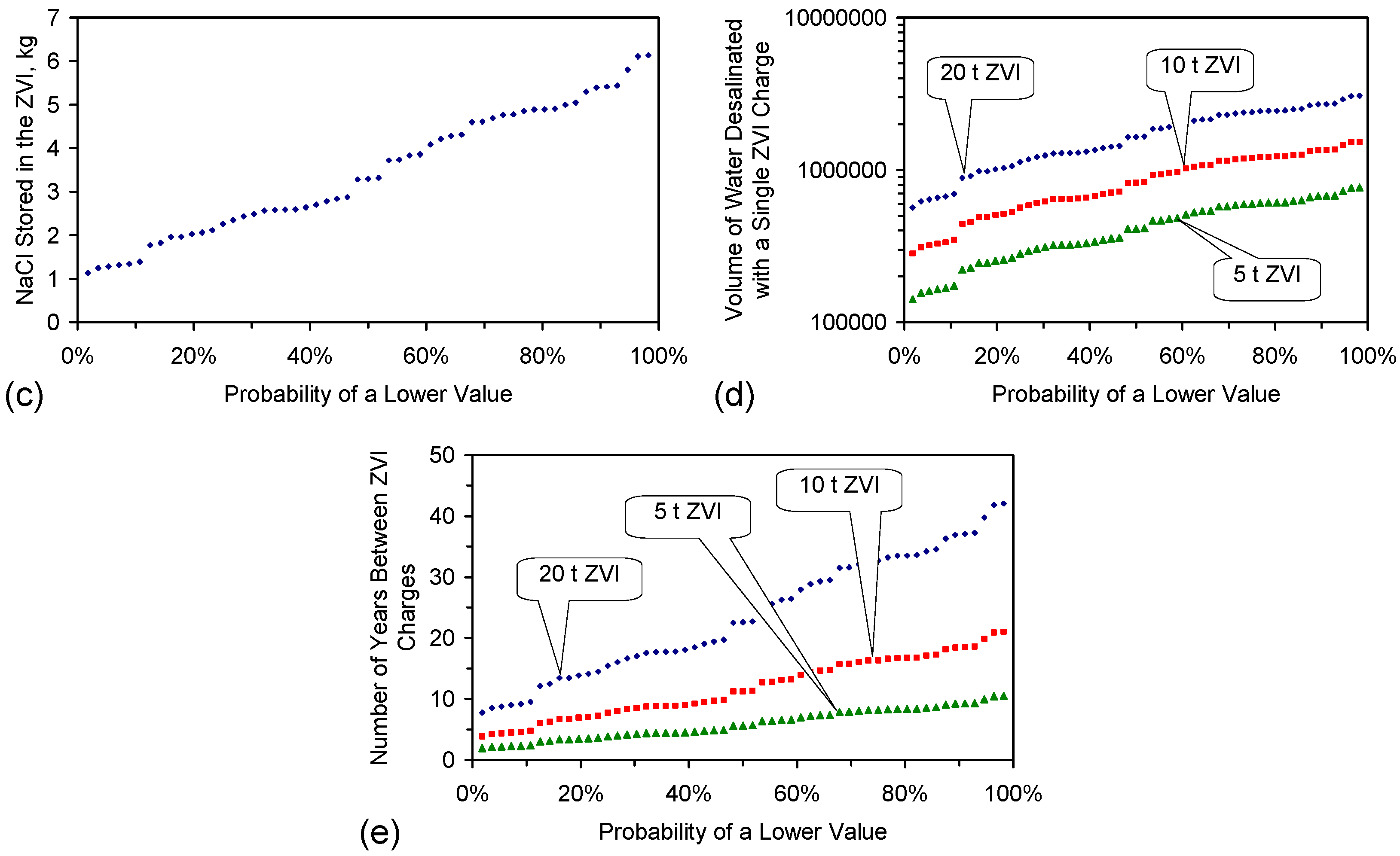
- The trial data demonstrates that the amount of NaCl removed per unit time is independent of the concentration of ZVI, g/L, Pw (Figure 17a,b);
- These trial observations indicate that:
- Each 1 g of ZVI will be expected to remove at least 0.35 g NaCl before it needs to be removed from the reaction environment and is replaced (Figure 17a–c).
- Scale up by the placement of 10 t ZVI in a saline aquifer would result in the removal of up to 3.5 t NaCl from the aquifer, before the replacement of the ZVI is required (Figure 17a–c). This experimental scale up allows:
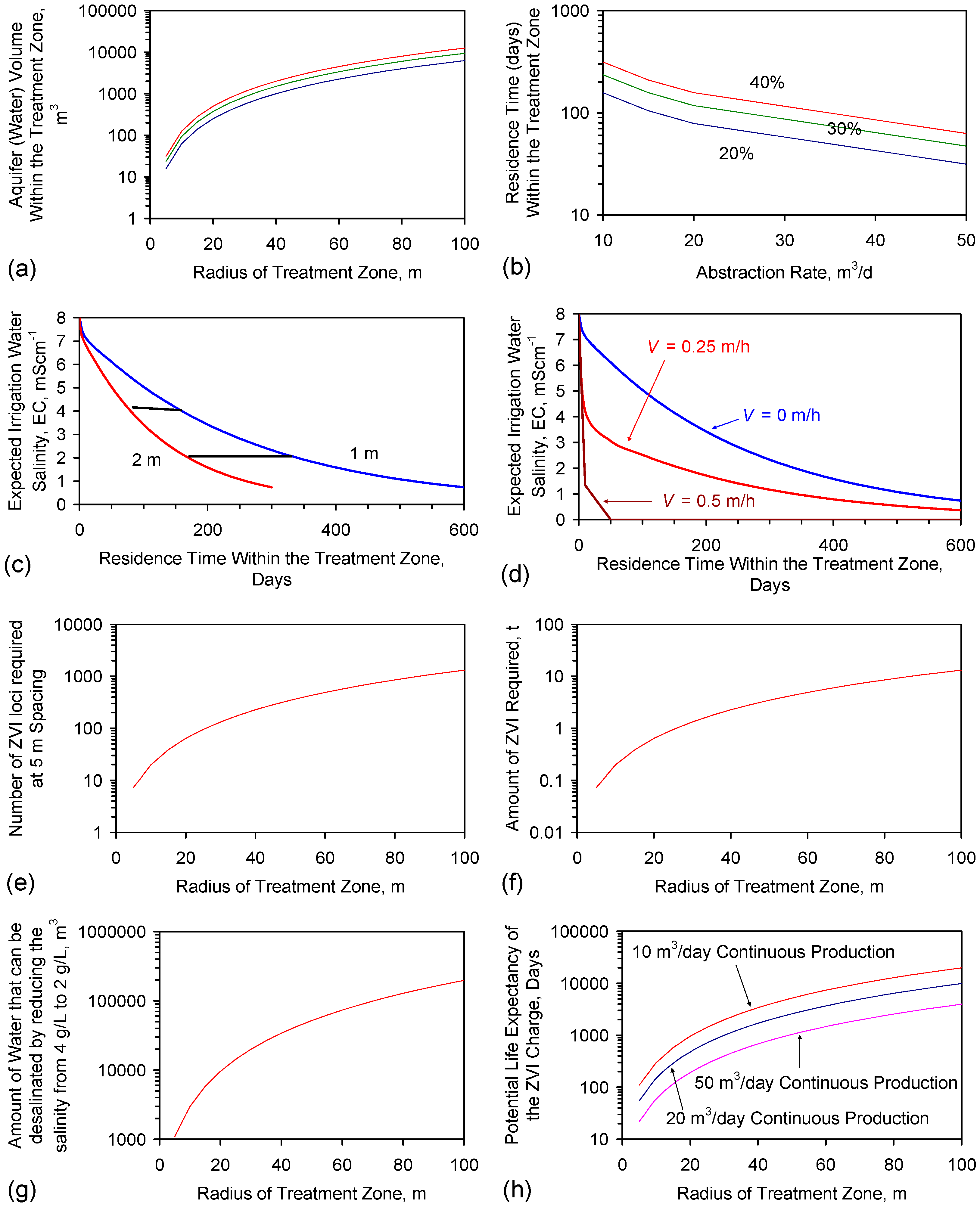
- Assessing from the trial data set, the size of the Aquifer Treatment Zone which is required to deliver the target volume of irrigation water:
- In a commercial development the ZVI will be placed in a number of loci (wells) which intersect the aquifer. The number of loci required is defined by the ZVI concentration data used in the trials (e.g., Figure 17a,b).
- The required residence time, td, to achieve the required irrigation water salinity is defined by the trials kinetic data (e.g., Equations (A1) to (A4); Figure B1, Figure B2 and Figure B3). The residence time is combined with the irrigation water volume required (Table 1) to define the minimum volume of water, and the minimum gross rock volume, contained within a proposed Aquifer Treatment Zone, Vaq (Equations (E1)–(E3) and (E5)).
- This minimum water volume is then integrated with the known aquifer properties in order to identify an aerial extent for the proposed Aquifer Treatment Zone Equation (E4).
7.3. Selection of Catalyst for the Proposed Aquifer Treatment Zone
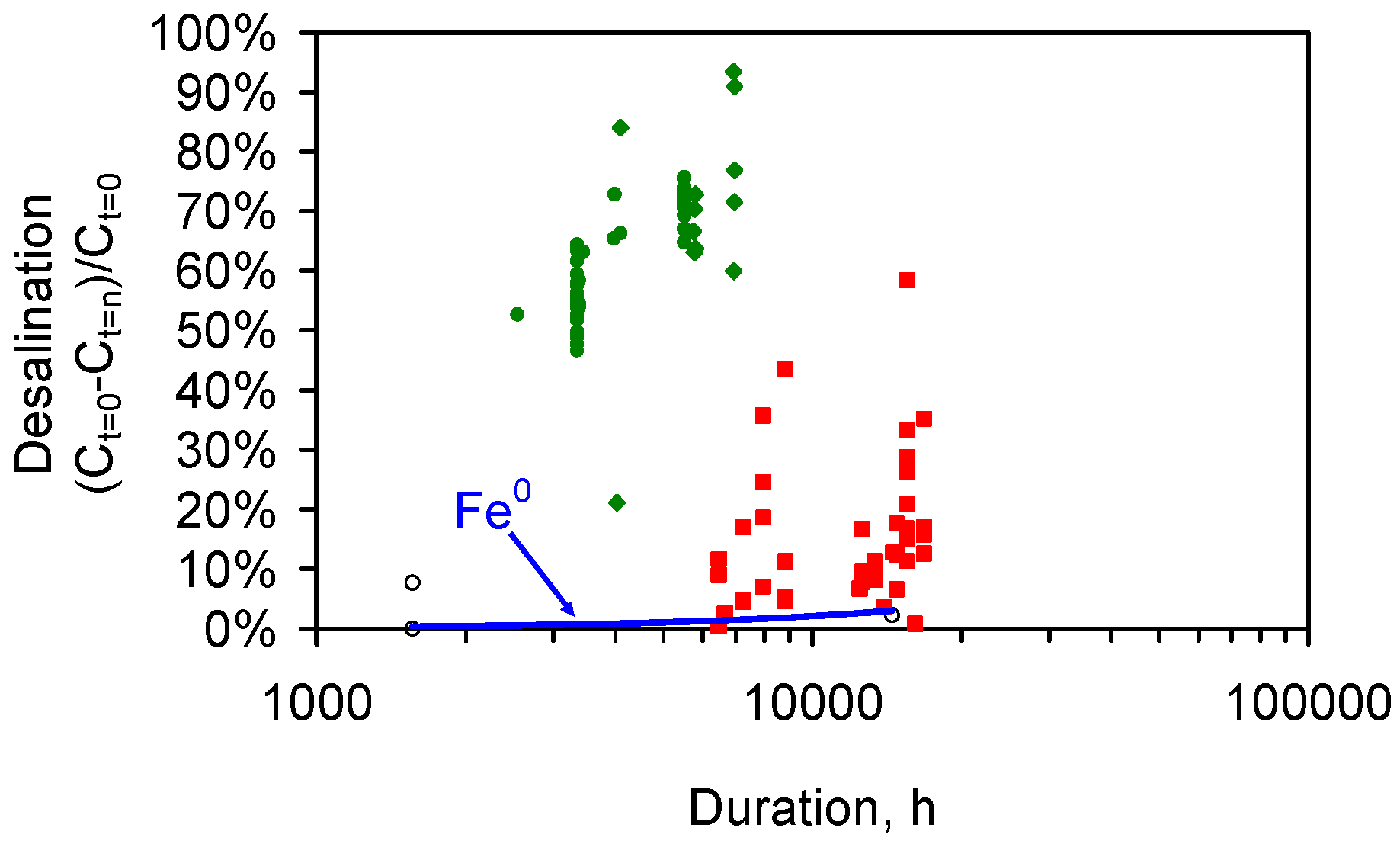
- A Type A Catalyst: This catalyst type (catalysts ST and MT) has a rigid porosity (Figure A2) and will, when placed in saline water, gradually remove NaCl from the water over a period of time (e.g., 100–1500 days). It has a low kr (Figure B1, Figure B2 and Figure B3) and a low BS. The irreducible (or equilibrium) salinity, BS, increases with decreasing catalyst porosity (Equations (8)–(14)). Fe0 powders, with no effective porosity, do not desalinate water (Figure B1) [36]. The statistical 1st and 3rd desalination quartiles for td = 200 days, for the three Type A catalysts considered in this study are: (i) ST catalyst (Figure A2; Figure B1, Figure B2 and Figure B3), 15 mm diameter pellet: 54.4% to 70.8%; n = 50; (ii) ST catalyst (Figure B3b), 75 mm diameter pellet: 63.2% to 76.8%; n = 13; (iii) MT catalyst (Figure B1), 20–25 mm diameter pellet: 6.1% to 13.7%; n = 24. The amount of NaCl that can be removed is controlled by the porosity (Equations (8)–(14)) and the amount of catalyst placed in the reaction environment (Figure 17). The Type A catalyst will require a residence time in the aquifer of 100–500 days before the maximum (design) equilibrium desalination is achieved (e.g., Figure F1, Figure F2 and Figure F3).
- A Type B Catalyst: This catalyst type (catalysts C to K) has an expandable, or poro-elastic, porosity (e.g., Table E1 and Table F1). The catalyst will, when placed in saline water, in a reaction environment incorporating water recycle, result in a relatively rapid removal of NaCl from water (e.g., 3 to 50 h). It has a high kr (Table E1 and Table F1) and a relatively high BS (e.g., 20%–80% (e.g., Table 1, item 4e)). It can preferentially remove Na+ or Cl− ions. Once an initial BS is achieved, or the water recycle ceases, desalination continues to progress at a substantially slower rate (e.g., Figure B1, Figure B2 and Figure B3). The Type B catalyst will require a residence time in the aquifer of 1–30 days before the maximum (design) equilibrium desalination (e.g., F4, F5).
- A Static Strategy: where the ZVI catalyst is placed in the aquifer and no water is recycled to the aquifer;
- A Recycle Strategy: where some of the product water is recycled back to the aquifer.
7.4. Control Hydrological Data and Models Required for the Proposed Aquifer Treatment Zone
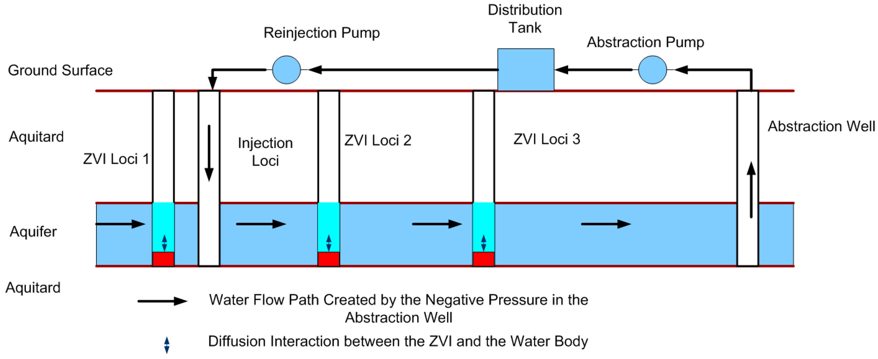
7.5. Construction of the Proposed Aquifer Treatment Zone Using the Static Strategy
- (a)
- a radial pattern of ZVI loci;
- (b)
- a single abstraction well located within the “Aquifer Treatment Zone” ;
- (c)
- an excess of ZVI is placed in each ZVI loci to increase the life expectancy of each ZVI charge. The life expectancy of a ZVI charge could be designed to exceed 20 years (Figure 17);
- (d)
- a simple process flow diagram (Figure 18);
- (e)
- a simple construction (Figure 19).
- (a)
- is suitable for most agricultural holdings;
- (b)
- can be installed using basic, simple, low cost, and widely available equipment and tools. Many of these tools may already be available on the agricultural holding, as the required augers are commonly used to install fence posts; and
- (c)
- requires no operating energy during its life (apart from power for the abstraction pump).
Costs Associated with the Static Strategy
7.6. Construction of the Proposed Aquifer Treatment Zone Using the Recycle Strategy
7.6.1. Poro-Elastic vs. Rigid Vo
- (i)
- catalyst D(i) = 8.4% to 13.7%, n = 31;
- (ii)
- catalyst D(ii) = 9.9% to 65.0%, n = 18.
7.6.2. Recycle Strategy
8. Commercial Scale-Up Risk
- Industrial Waste Water Treatment Plant, Shanghai: processing 60,000 m3/day [83,84]. A number of 2 h duration pre-development batch flow trials (containing 0.5 kg Fe0) were undertaken [83]. They were succeeded by a single continuous flow pre-development trial (containing 40 kg Fe0) at a rate of 120 L/d [83]. This pilot trial was operated for 6 months prior to commercialization [83]. The throughput scale-up factor was 500,000. The scale-up factor in the amount of Fe0 used was 22,950.
9. Comparative Desalination Cost Structure
10. Conclusions
10.1. The Static Strategy
10.2. The Recycle Strategy
10.3. Dual Use Strategy
10.4. Next Stage
Acknowledgments
Author Contributions
Conflicts of Interest
Appendix A. Trial Materials and Kinetic Methodology
A1. ZVI


A2. Microscopy
- (i)
- divisions at 0.15 mm, 0.1 mm, 0.07 and 0.01 mm supplied by No. 1 Microscope Wholesale Store, Henan, China, and
- (ii)
- divisions at 0.01 mm supplied by United Scope (Ning Bo) Co Ltd. Zhejiang, China.
A3. Saline Water Construction
A4. Water Analyses
- (i)
- ORP (oxidation reduction potential);
- (ii)
- pH;
- (iii)
- electrical conductivity (EC);
- (iv)
- temperature.
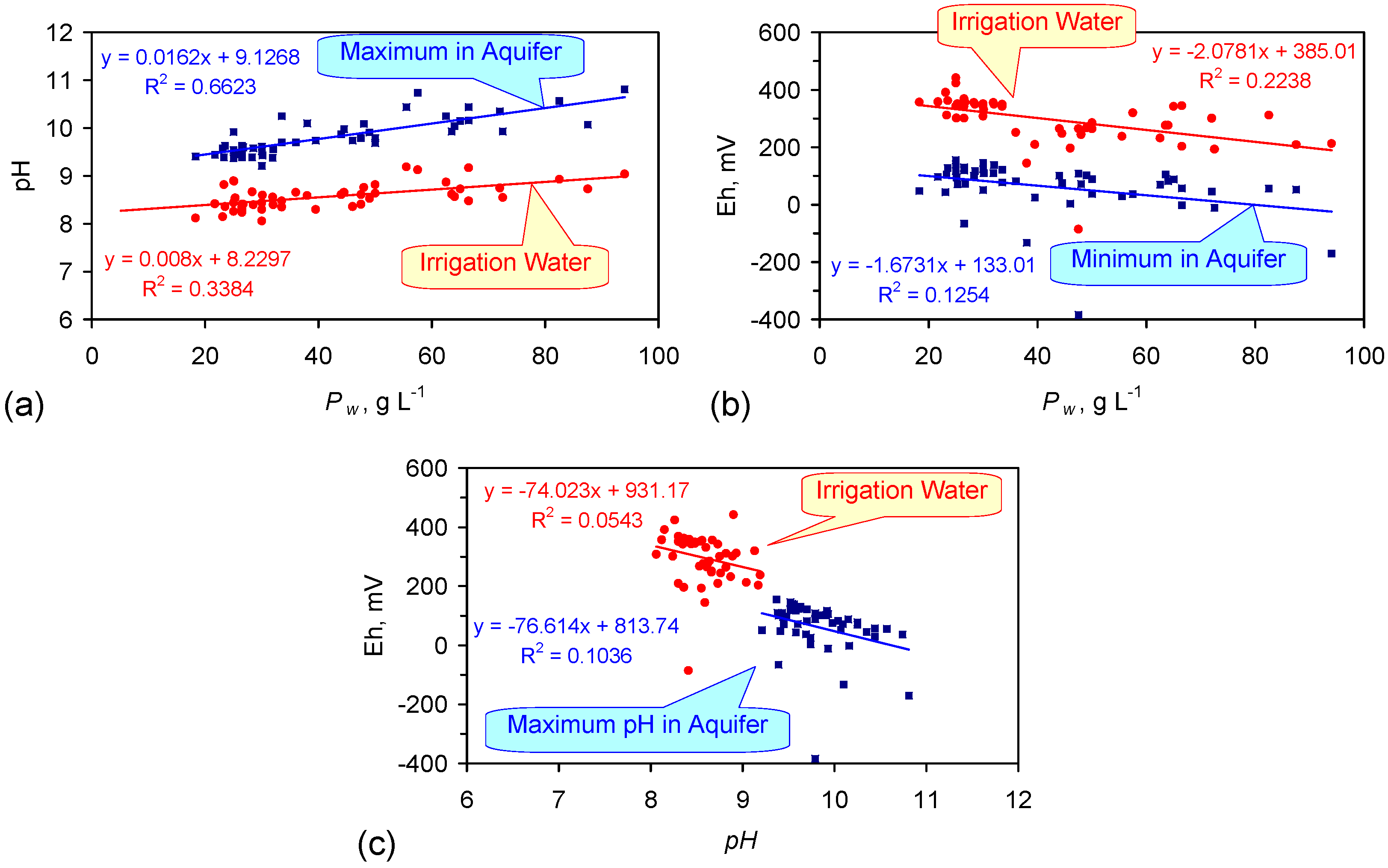
A4.1. pH
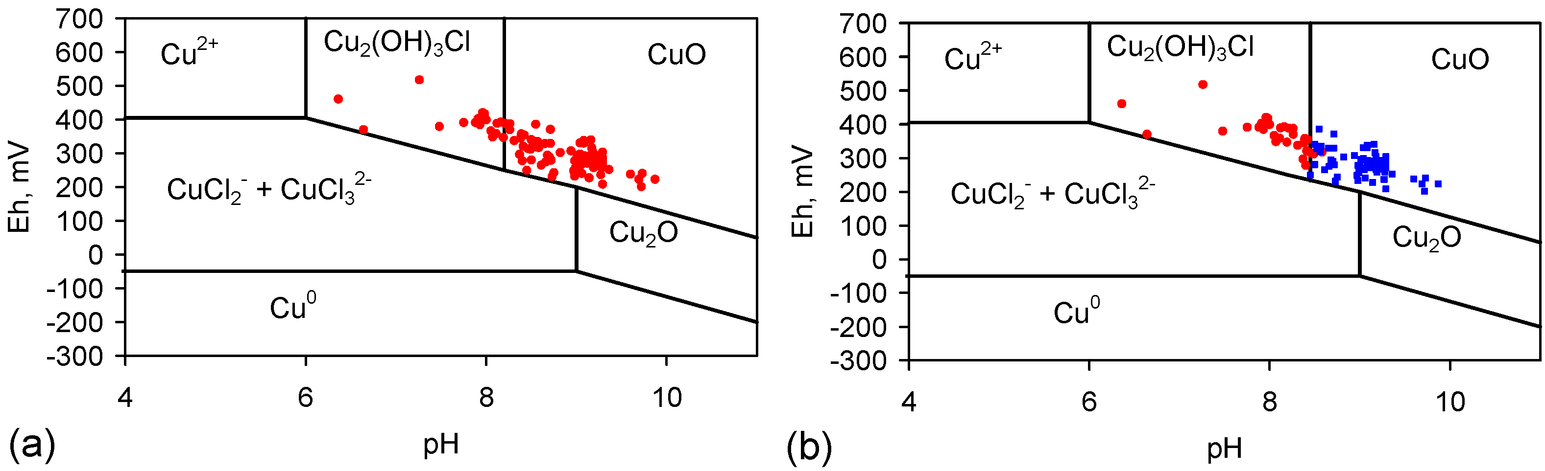
A4.2. Eh
A4.3. EC (Electrical Conductivity)
A4.4. Na+ and Cl− Ion Concentrations
A4.5. Temperature
A5. Reactor
A6. Pellets and Cartridges
A7. Conversion of Batch Flow Kinetic Data to Continuous Flow Kinetic Data
Appendix B. Kinetic Data Associated with ST Series Desalination Pellets
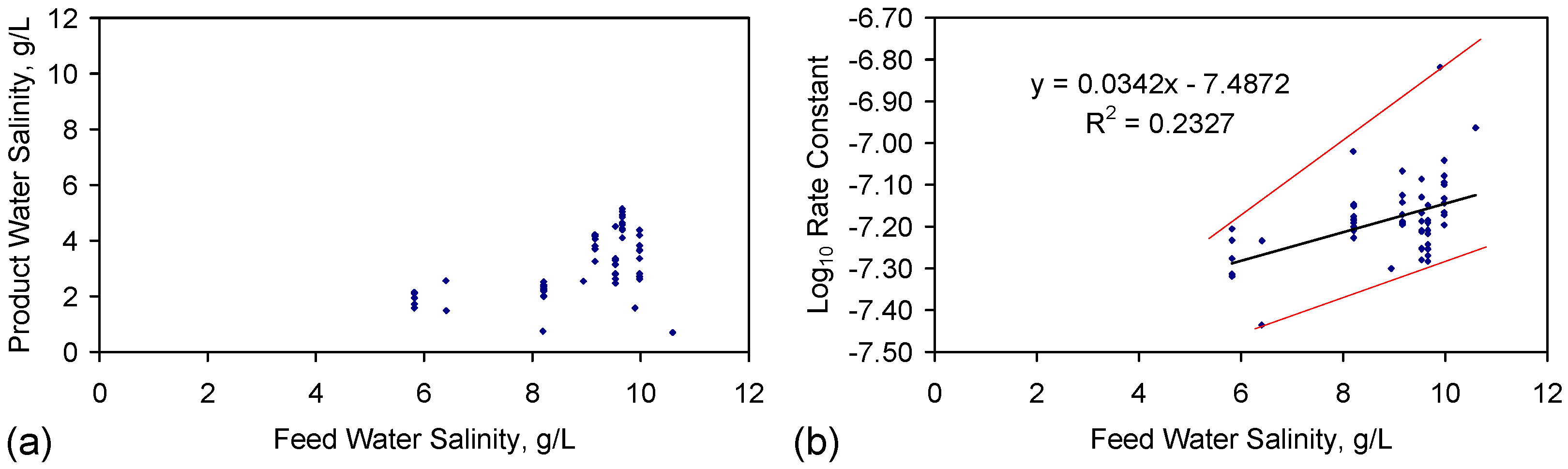
B1. Desalination Rate Constant
- (a)
- (b)
- (c)
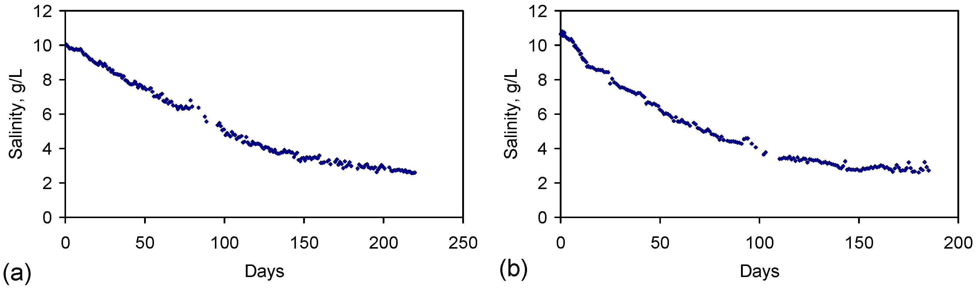
- Salinity (Ct = n) measured as a function of time t, follows the general decline pattern of a first order reaction (Figure B3).
B2. Desalination Pellet Dimensions
- the composition of the impermeable pellet sheathing material does not affect the rate of desalination, or the amount of desalination that can occur. The ability to use MPDE (or an alternative) as a sheathing material (instead of copper) substantially reduces the pellet cost. Suitable alternatives include: (i) ABS: acrylonitrile-butadiene-styrene; (ii) Buna-N: Copolymer of butadiene and acrylonitrile; (iii) CPVC: chlorinated polyvinyl chloride; (iv) EPDM: Ethylene-propylene-diene monomer; (v) FPM: Fluoro-carbon elastomer; (vi) GRP: Glass reinforced plastics; (vii) HDPE: high density polyethylene; (viii) PA 11: polyamide 11; (ix) PB: polybutylene; (x) PE: polyethylene; (xi) PEX: cross-linked polyethylene; (xii) PIR: polyisocyanurate; (xiii) PK: polyketone; (xiv) PP: polypropylene; (xv) PTFE: polytetrafluoroethylene; (xvi) PVC: polyvinyl chloride; (xvii) PVDF: poly vinylidene fluoride; (xviii) PVP: polyvinylpyrrolidone; (xix) SBR: styrene-butadiene;
- pellets with diameters of 15 mm, 20 mm, 25 mm, 40 mm and 75 mm are effective;
- the pellets can have one, or two, open ends, which are in contact with the water body;
- individual pellets can be structured with lengths of more than 0.5 m;
- desalination continues to occur when air and water temperatures drop below 0 °C [16].
Appendix C. Equations and Models Which Are Required to Provide a Control Data Set for the Aquifer and to Provide Effective Monitoring of a Proposed Aquifer Treatment Zone Following Installation
C1. Flow Rate and Iso-Potential Modelling
C1.1. Simple Reconstruction of an Aquifer
- a single abstraction well to be used to provide water for irrigation;
- The abstraction pump creates a point source with a negative head (sink) [75];
- the abstraction well is surrounded by a number of point loci (e.g., infiltration devices, wells, boreholes) containing ZVI pellets or cartridges.

C1.2. Identification of Heterogeneity in the Proposed “Aquifer Treatment Zone”

C2. Assessment of the Size of a Proposed Aquifer Treatment Zone
C2.1. Hydrological Parameters Associated with a Proposed Aquifer Treatment Zone
- at t = 0, the porosity contains mobile water + irreducible (bound) water;
- at t = n, following drawdown, the porosity can contain mobile water + irreducible water + mobile air + irreducible air.
C2.1.1. Radial Area of Influence of the Abstraction Well
C2.1.2. Volume Influenced by the Abstraction Well during a Control Pump Trial
C2.1.3. Flow Rate at Each Loci

C2.2. Complex Treatment of Under-Saturated Flow
C3. Hydrological Issues Associated with the Placement of ZVI in an Aquifer
C3.1. ZVI Permeability
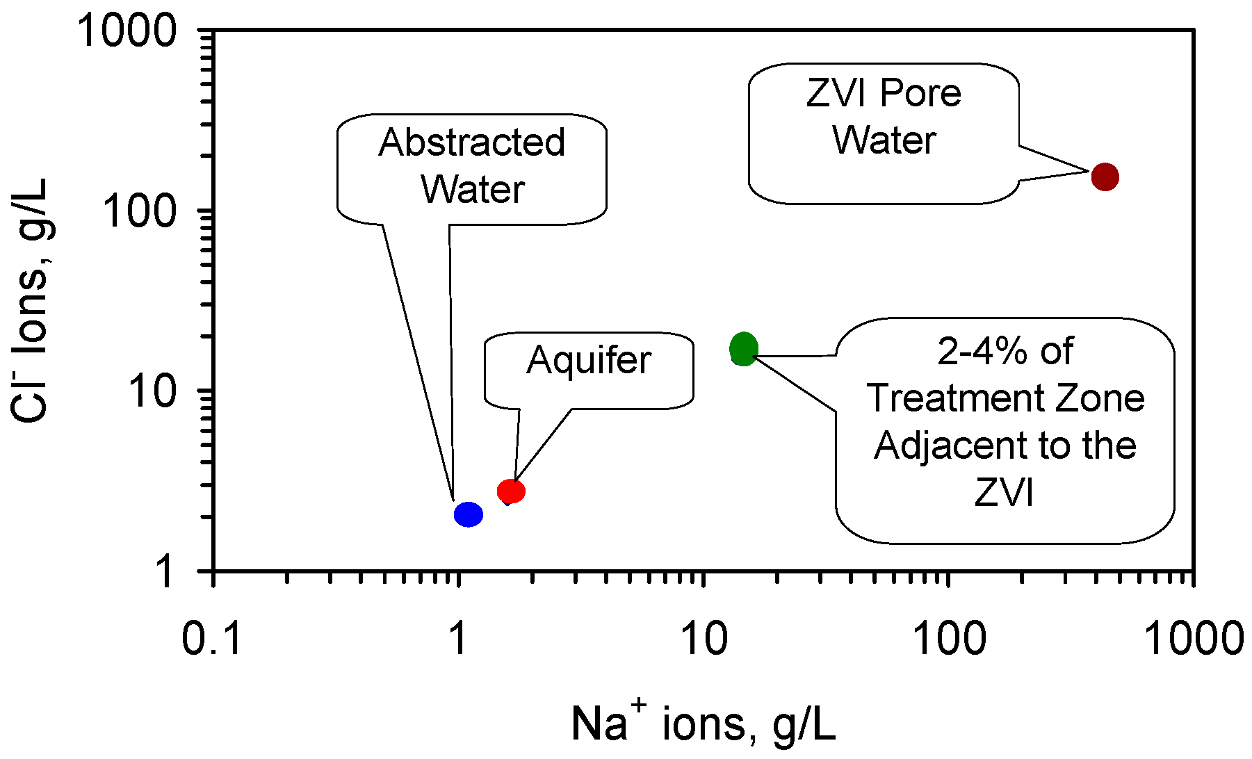
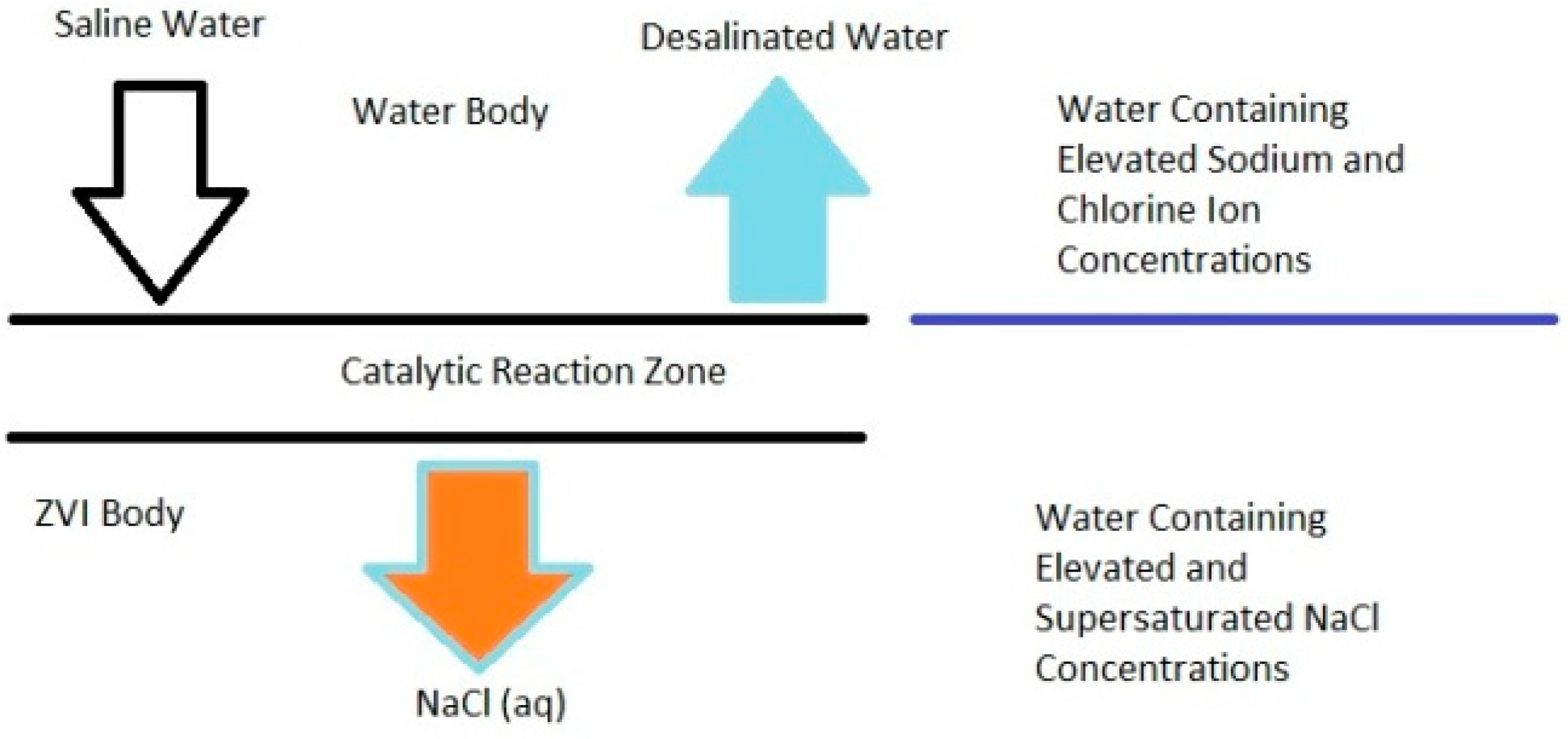
C3.2. Haloclines: Interaction between the ZVI Loci and the Surrounding Aquifer
- (a)
- zone of super saturation of NaCl within the ZVI pellets;
- (b)
- (c)

C4. Modeling Diffusion Fluid Flows Which Affect the Water Salinity
C4.1. Diffusion Flow Analysis
C4.2. Non-Fickian Diffusion Flow
- (i)
- the fluid velocity (V) is constant, and
- (ii)
- the only direction of flow is towards the abstraction well, e.g., [144]:δ(c2)/δt = −V·δ(c2/δx) + D·δα(c2)/δxα
C5. Space Velocity
C6. Mineral Precipitation, Gas Occlusion, and Biofilms within the Aquifer
C6.1. Impact of Mineral Precipitation and Gas Discharge from the ZVI on Aquifer Permeability

C6.2. Estimating Permeability Changes Due to Mineral Precipitation and Gas Occlusion
C6.3. ZVI Gas Generation
C6.4. Biofouling, Biofilms
Appendix D: Classifying the Potential Aquifer Resource
- Prospective resource;
- Contingent resource;
- Developed resource.
D1. Prospective Resource
- Play: Shallow aquifer which is believed to extend under the proposed Aquifer Treatment Zone ground surface but has not been demonstrated to be present by drilling or by the insertion of wells.
- Lead: Shallow aquifer whose presence has been identified by one or more wells or infiltration devices, but requires more data acquisition before it can be deemed to be suitable for conversion to an Aquifer Treatment Zone.
- Prospect: Shallow aquifer which has been identified and has been partially defined, but is insufficiently defined to represent a viable Aquifer Treatment Zone target.
D2. Contingent Resource
- Development Pending: Requires further data acquisition (aquifer, hydro/geochemical, regulatory, crop economics) and/or evaluation (financing, insurance, regulatory, crop analysis) in order to confirm commerciality;
- Development on Hold: Awaiting changes in market conditions (e.g., crop prices) or removal of other constraints to development (e.g., political, regulatory, financing, insurance, customers, seed availability, etc.);
- Development not Viable: No current plans exist to develop the defined resource or acquire additional data at this time due to aquifer constraints, legal, regulatory, chemical, commercial, insurance, crop, political, environmental issues, or one or more other constraints. A development site which is not viable at a specific time may become viable if one or more of the underlying constraints changes.
D3. Developed Resource
- On Production: The Aquifer Treatment Zone has been installed and is in operation producing partially desalinated water;
- Under Development: All necessary approvals and consents have been obtained, and construction of the Aquifer Treatment Zone is underway;
- Planned for Development: The project satisfies all technical constraints, and there is a firm intent from the land owner to progress with the installation of an Aquifer Treatment Zone. Installation is being held up by one or more of detailed development planning, regulatory, financing and insurance approvals, and contracts finalization.
Appendix E. Calculating and modeling the Dimensions Associated with a Proposed Aquifer Treatment Zone
E1. Area of Influence of Each ZVI loci Placed within an Aquifer
E2. Sizing the Aquifer Treatment Zone
E3. Sizing Identifying the Ground Surface Area Which Overlies the Aquifer Treatment Zone
E4. The Required Aquifer Gross Rock Volume
E5. Assessment of the Significance of Catalyst Selection on the Number of ZVI Loci Required

| Trial Group | Reactor Size, L | Pw, g Fe0/L | Sub-Optimised Rrc | Optimised Rrc | A0, g/L | At = n, g/L | Rrt, h | Log10 (kobserved) | Log10 (kactual) | Water Volume Treated, L | Scale-Up Required to Achieve 20 m3/day | Scale-Up Required to Achieve 20 m3/day with Optimised Operation |
|---|---|---|---|---|---|---|---|---|---|---|---|---|
| RC1 | 5.8 | 23.28 | 3.60 | 2.48 | 4.21 | 3.03 | 5.80 | −4.80 | −6.17 | 63.8 | 833.3 | 574.7 |
| RC2 | 240.0 | 0.50 | 11.08 | 3.00 | 2.97 | 2.14 | 22.15 | −5.39 | −5.09 | 12000.0 | 76.9 | 20.8 |
| RC3 | 8.0 | 28.00 | 20.25 | 1.35 | 2.65 | 0.79 | 45.00 | −5.13 | −6.57 | 32.0 | 4687.5 | 312.5 |
| RC4 | 5.8 | 8.79 | 302.28 | 7.45 | 4.25 | 2.81 | 487.00 | −6.63 | −7.57 | 34.8 | 69,971.3 | 1724.1 |
| RC5 | 5.8 | 4.80 | 11.75 | 3.10 | 36.17 | 25.71 | 18.93 | −5.30 | −5.98 | 92.8 | 2719.8 | 718.4 |
| RC6 | 5.8 | 0.86 | 12.22 | 3.72 | 15.66 | 8.67 | 19.68 | −5.08 | −5.01 | 75.4 | 2827.6 | 862.1 |
| RC7 | 5.8 | 4.66 | 9.62 | 3.10 | 8.84 | 7.04 | 15.50 | −5.39 | −6.06 | 29.0 | 2227.0 | 718.4 |
| RC8 | 5.8 | 0.86 | 2.84 | 1.86 | 6.46 | 5.30 | 4.58 | −4.92 | −4.86 | 17.4 | 658.0 | 431.0 |
| RC9 | 800.0 | 0.07 | 3.21 | 0.45 | 2.10 | 1.28 | 42.74 | −5.49 | −4.34 | 9600.0 | 44.5 | 6.3 |
Appendix F. Concepts and Models Associated with a Recycle Strategy
F1. Engineering Concepts Associated with Catalytic Recycle
F1.1. Modelling the Recycle Water Flow Rate (V)
- (a)
- reinjected into the aquifer within the proposed Aquifer Treatment Zone, or
- (b)
- recirculated within the proposed Aquifer Treatment Zone.
- (i)
- (ii)
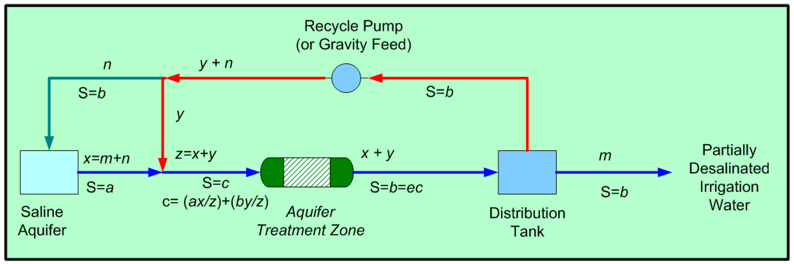
- The volume of abstracted water, which is radially reinjected into the Aquifer Treatment Zone at a distance rinj from the abstraction well is denoted as y m3/d (Figure 20).
- (iii)
- The volume of water, which is used for irrigation = m (Figure 20).
- (iv)
- The volume of water present in a confined (or closed) proposed Aquifer Treatment Zone during recycle is WTZ1.
F1.2. Closed Environment
F1.3. Recycle Loop
F2. Primary Engineering and Hydrological Concepts Associated with Catalytic Recycle
F2.1. Semi-Closed Aquifer Treatment Zone With Aggressive Recycle
- (i)
- a strong negative potential being created by the abstraction well, and
- (ii)
- a dispersed, low positive potential being associated with reinjection, (or infiltration), of the recycle water on the periphery of the Aquifer Treatment Zone.
- (i)
- by matching the net fluid outflow from the system for irrigation water, with
- (ii)
- a dispersed inflow around the treatment zone periphery by fresh saline water from the aquifer.
- (i)
- the recycle ratio can be reduced;
- (ii)
- the number of ZVI loci and infiltration loci can be reduced;
- (iii)
- the volume of water contained within the aquifer treatment zone can be reduced.
- (i)
- the ZVI requirement;
- (ii)
- the number of ZVI loci;
- (iii)
- the amount of desalination;
- (iv)
- the reinjection/reinfiltration requirement;
- (v)
- the size of the Aquifer Treatment Zone;
- (vi)
- the amount of irrigation water which can be abstracted from a specific Aquifer Treatment Zone Volume.
| Trial Group | Aquifer Volume, m3 | Irrigation Water (without Optimisation), m3·day−1 | Recycle Water, m3·day−1 | Optimised Irrigation Water, m3·day−1 | Feed Water Salinity, g·L−1 | Product Water Salinity, g·L−1 | Mean Desalination | Mean Na+ Removal | ZVI Required, t | Catalyst |
|---|---|---|---|---|---|---|---|---|---|---|
| ST | 4000 | 20 | 0 | 20 | 4.00 | 1.84 | 54.0% | 54.0% | 120 | ST |
| RC1 | 4000 | 16,552 | 59,586 | 24,000 | 4.00 | 2.88 | 28.0% | 93.12 | C | |
| RC1a | 4000 | 18,113 | 65,208 | 4.00 | 2.88 | 28.1% | 38.9% | 93.12 | ||
| RC2 | 4000 | 4334 | 48,000 | 16,000 | 4.00 | 2.88 | 27.9% | 2.00 | D | |
| RC3 | 4000 | 2133 | 43,200 | 32,000 | 4.00 | 1.19 | 70.2% | 112.00 | E | |
| RC4 | 4000 | 197 | 59,586 | 8,000 | 4.00 | 2.64 | 33.9% | 35.16 | F | |
| RC5 | 4000 | 5071 | 59,586 | 19,200 | 4.00 | 2.84 | 28.9% | 19.20 | G | |
| RC6 | 4000 | 4878 | 59,586 | 16,000 | 4.00 | 2.21 | 44.6% | 3.44 | H | |
| RC7 | 4000 | 6194 | 59,586 | 19,200 | 4.00 | 3.19 | 20.4% | 18.64 | I | |
| RC8 | 4000 | 20,961 | 59,586 | 32,000 | 4.00 | 3.28 | 18.0% | 3.44 | J | |
| RC9 | 4000 | 2246 | 7,200 | 16,000 | 4.00 | 2.43 | 39.3% | 0.28 | K | |
| RC9a | 4000 | 9600 | 7,200 | 4.00 | 2.41 | 39.6% | 50.6% | 0.28 |
F3. Modeling of Catalytic Recycle
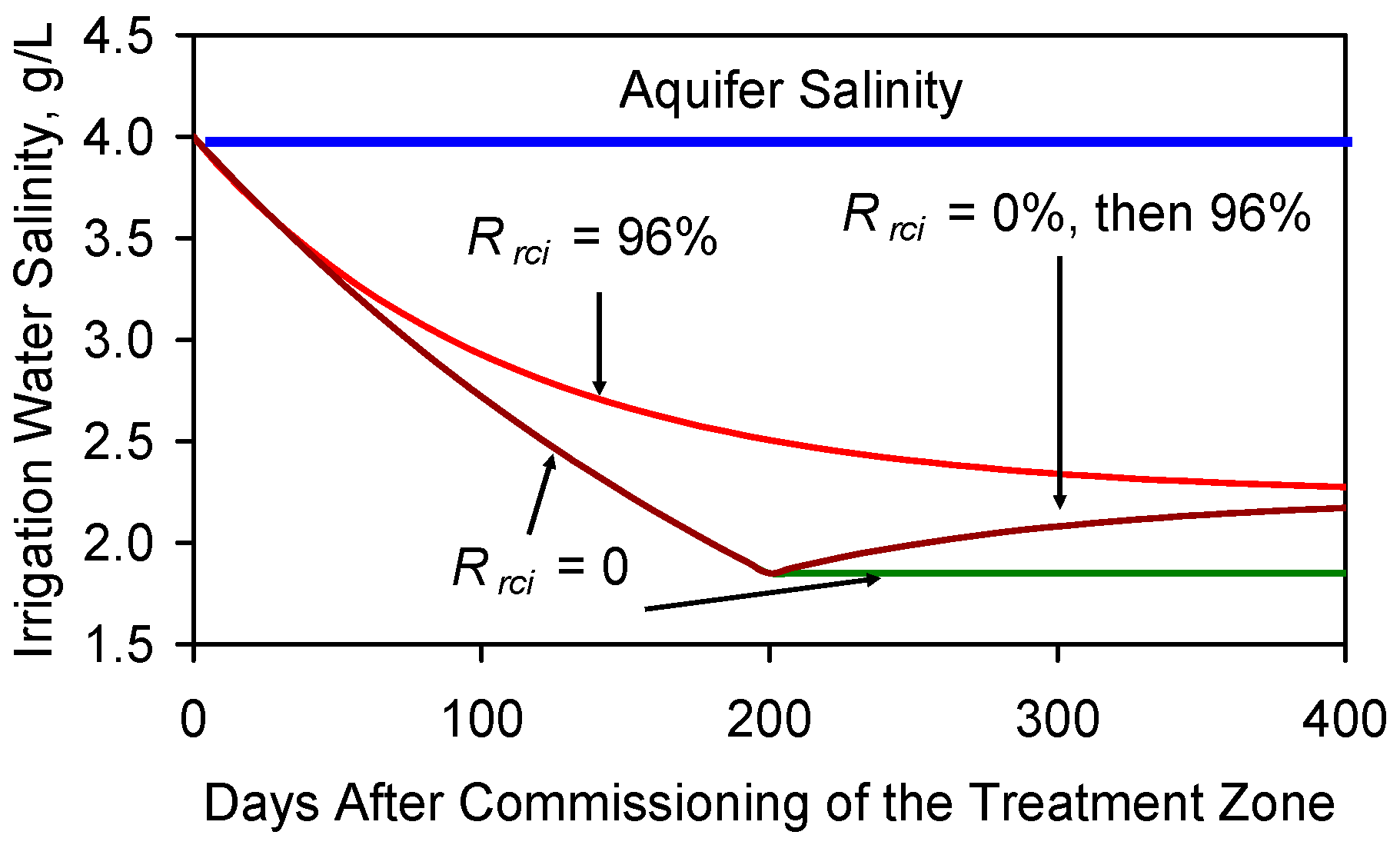
F3.1. Desalination Without Recycle: Type A Catalyst
- (i)
- a 60 m radius around the abstraction well,
- (ii)
- 20 m3·day−1 abstraction (without recycle, i.e., y = 0 m3·day−1; m = x = 20 m3·day−1,
- (iii)
- td = 200 days,
F3.2. Desalination With Recycle: Type A Catalyst
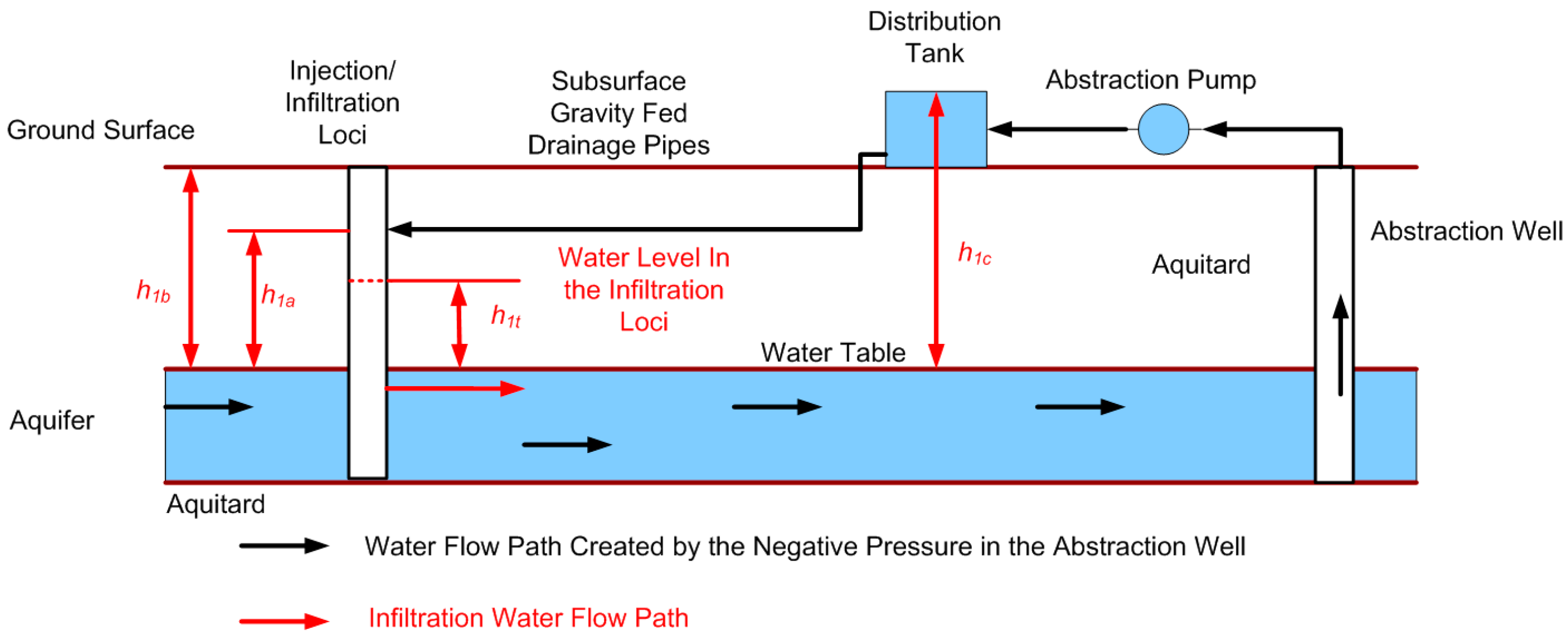
F4. Hydrological Issues Associated with the Reinjection Loci
F4.1. Gravity Fed Reinjection Sites
F5. Desalination Issues Associated with Recycle
F5.1. Impact of Increasing the Aquifer Abstraction Rate without Recycle
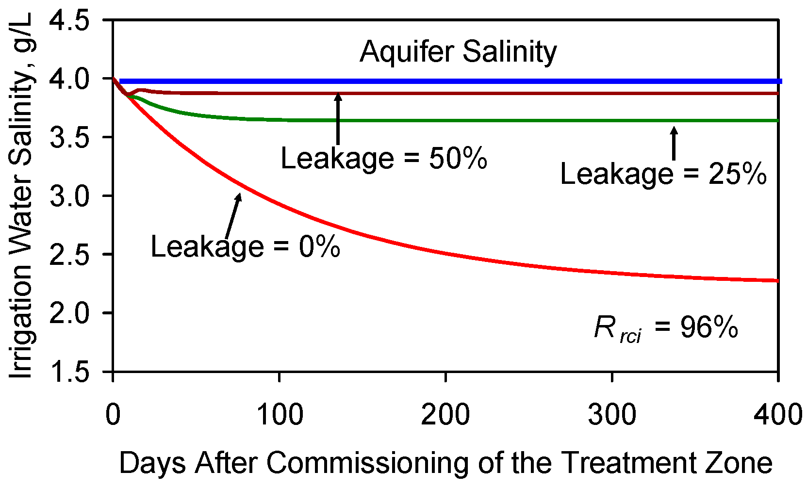
F5.2. Impact of Different Recycle Strategies
F5.3. Impact of Leakage of Reinjected Water to the Principal Aquifer
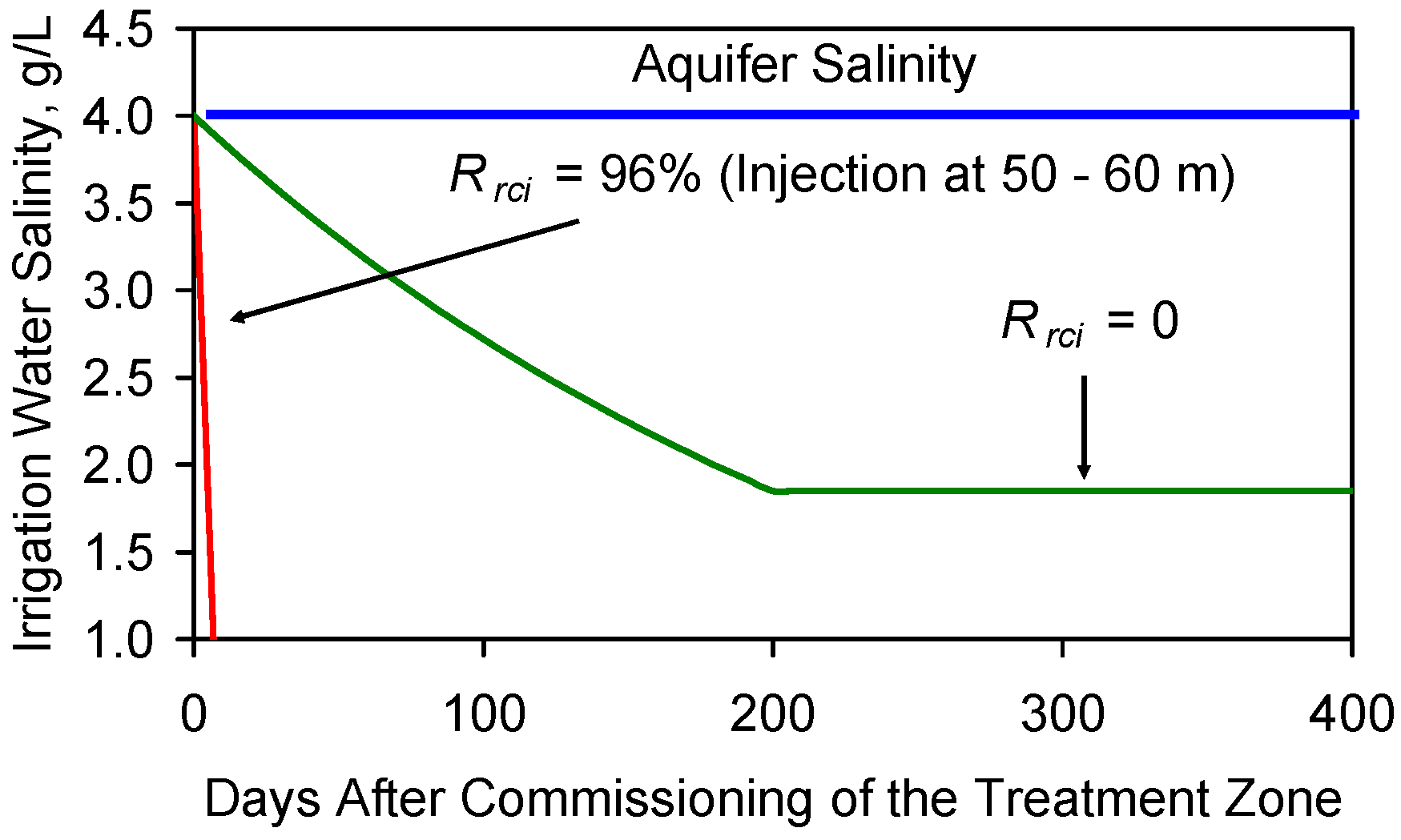
F6. Impact of Changing Reinjection Location on Desalination
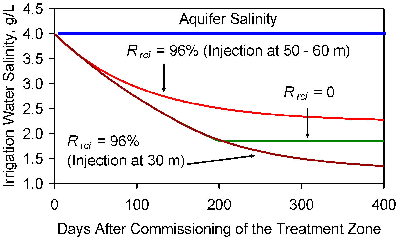
F6.1. Placement of the Injection Loci within the Aquifer Treatment Zone
- 50–60 m from the abstraction well (4524 m3 water volume), and
- the injection loci are 30 m from the abstraction well (1131 m3 water volume),

F7. Impact of Catalyst on Desalination
F7.1. Impact of Changing the Rate Constant
- (1)
- decrease c2 (and increase kr), unless
- (2)
- the increase in V is matched by a corresponding increase in the dispersion coefficient D (Equation (C21)).
- (i)
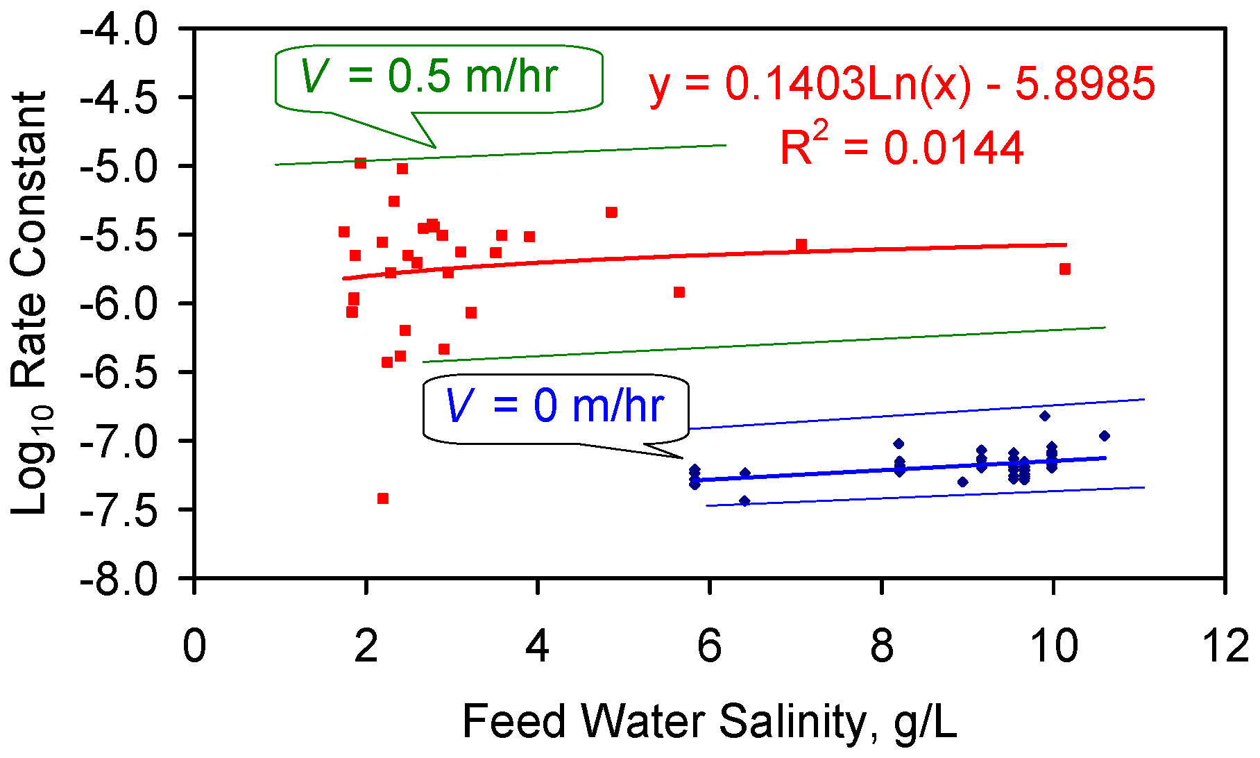
- reinjection at the periphery of the Aquifer Treatment Zone without leakage, (with the desalination rate constants (for V = 0.5 m/h) will result in (D − V) decreasing as V increases;
- (ii)
- suitable catalyst design (combined with reinjection) may allow the residence time required to reduce the water salinity to the required level to be substantially reduced, relative to a base case with no reinjection (Figure F4).
F7.2. Equilibrium or Base Salinity Level
Appendix G. Modeling Aquifer Heterogeneity, Static Strategy
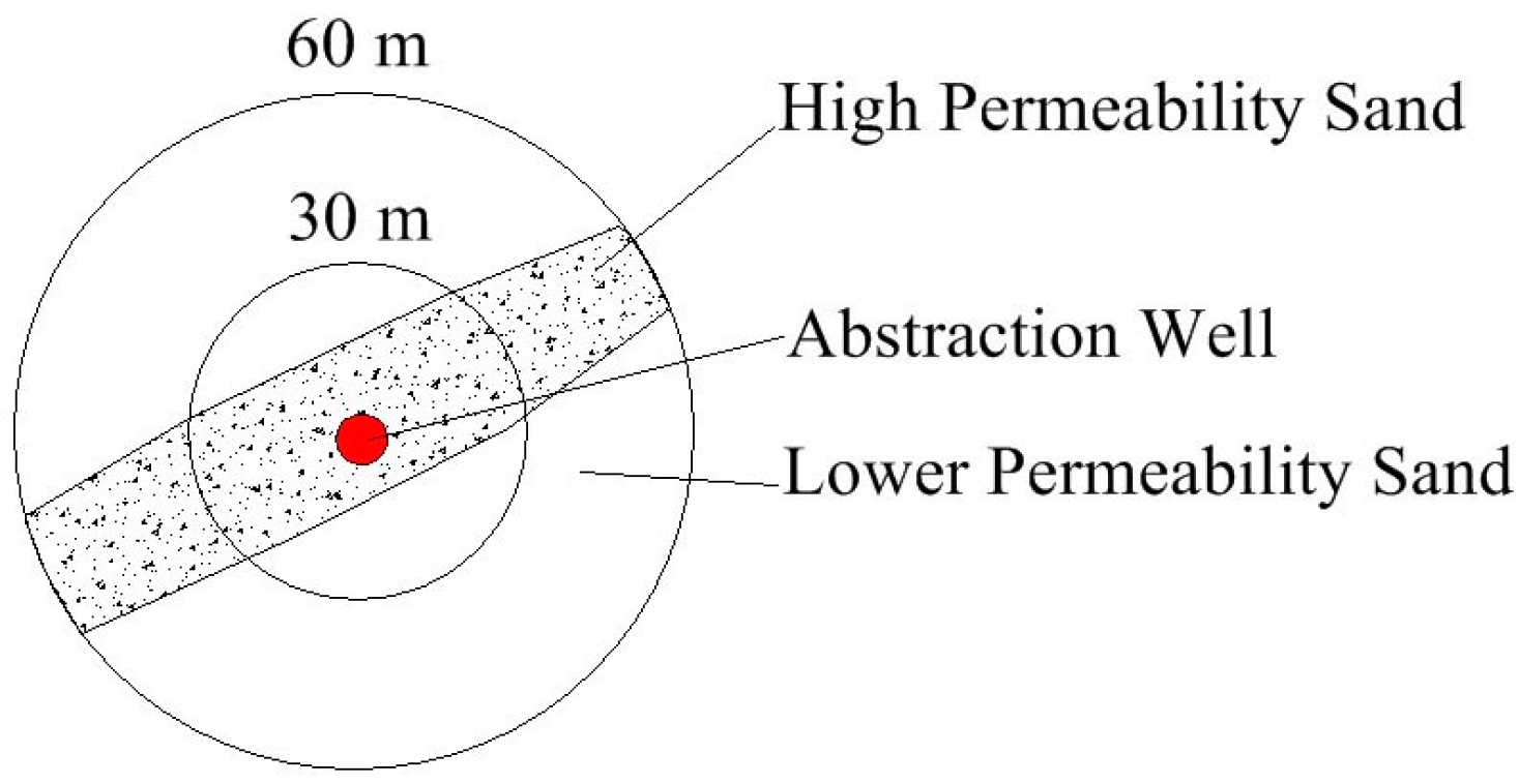
G1. Impact of Geology on Desalination
- (i)
- increase differential flow from the aquifer to the abstraction well through the Aquifer Treatment Zone;
- (ii)
G2. Impact of Permeability Variation within the Aquifer

- (i)
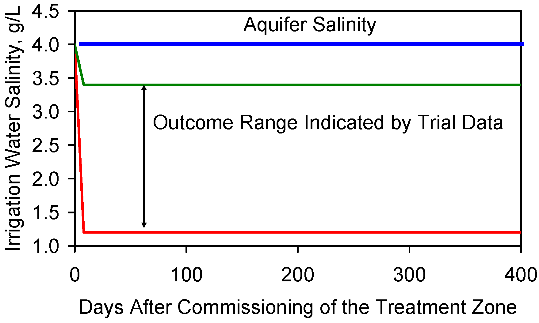
- The initial design of the aquifer (based on the lower permeability aquifer) will assume that the average residence time is 200 days (based on a 20 m3·day−1 abstraction rate).
- (ii)
- The presence of the higher permeability sand will result in an average residence time within this higher permeability sand of 20 days. This will result in about 80% of the abstracted water being derived from this sand. The remaining 20% will be derived from the lower permeability sand.
- (i)
- water arriving at the abstraction well from both the lower permeability aquifer and the higher permeability sand;
- (ii)
- the water contribution to abstraction well from the higher permeability sand will be 16 m3·day−1; salinity (ch) = 3.7 g·L−1;
- (iii)
- the average equilibrium residence time of the water within the lower permeability sand increasing to 814 days (based on 3256 m3 water volume in the lower permeability sand and a 4 m3·day−1 abstraction rate); salinity (cl) = 0.17 g·L−1;
G3. Assessing the Relative Contribution of Different Water Sources
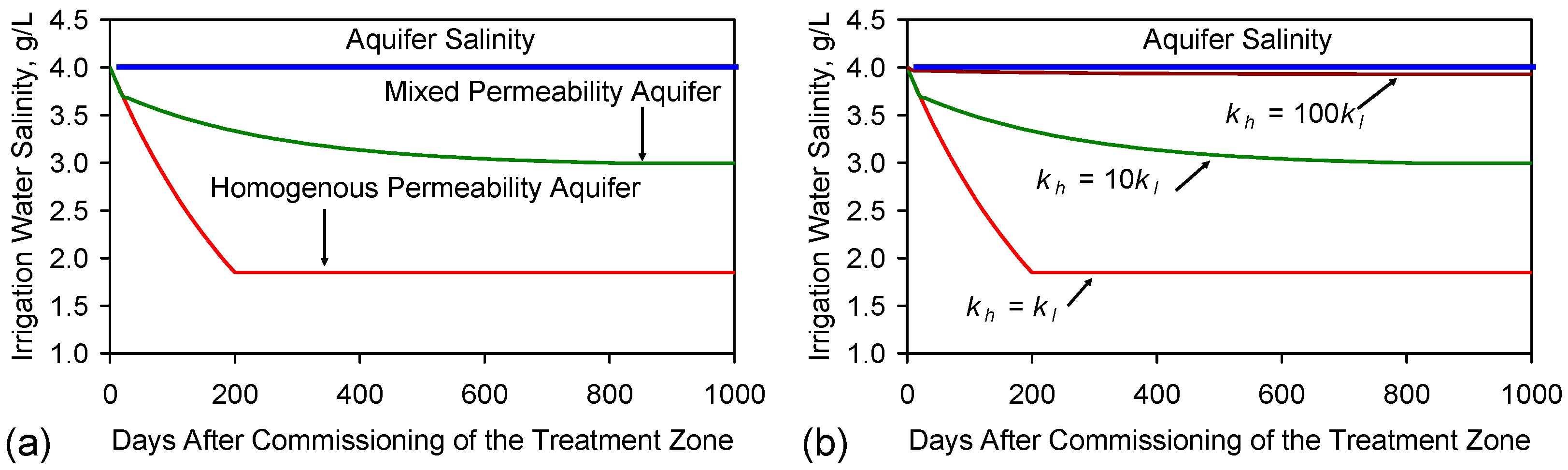
G4. Impact of Differential Permeability Variation (and Flow by-Pass) within the Aquifer
- (i)
- (ii)
- a series of higher permeability discrete lenses [185] within the treatment zone. This results in the effective by-pass of some of the surrounding lower permeability aquifer [185]. The net result of this change is to increase the equilibrium abstracted water salinity (when compared with a homogenous aquifer). The exact changes will be location specific, but the general trend expected is demonstrated in Figure G2b.
Abbreviations and Symbols
| A | cross-sectional area of the flow pathway; |
| A | anion in chemical equations; |
| Ac | actual cost of supplying the partially desalinated irrigation water, $/m3; |
| Ar | aromatic chemical with an OH group; |
| AR | required abstraction rate, m3·day−1; |
| AT | Net water column thickness in the aquifer, m; |
| AV | required aquifer volume, m3; |
| Ainf | area of the base of the infiltration device, m2; |
| Asinf | area of the sides of the infiltration device, m2; |
| [A] | NaCl, or Cl−, or Na+ concentration at time t = n; |
| [Ao] | NaCl concentration at time t = 0; |
| a | fractional yield change due to fertilizer application; |
| a | a constant (Equation (26)); |
| a1 | plants per hectare; |
| as | normalized surface area of ZVI particle, m2·g−1. |
| asi | particle size, e.g., nm, mm; |
| BS | irreducible salinity; |
| b | fractional yield change due to fungicide application; |
| b1 | seed pods, or grain heads, or fruit per plant; |
| Ct=0 | feed water salinity at time t = 0; |
| Ct=n | product water salinity at time t = n; |
| C0 | aquifer water salinity; |
| CR | recycle water salinity. |
| CS | water salinity entering the Aquifer Treatment Zone; |
| c | fractional yield change due to pesticide application; |
| c2 | concentration of [A] where ([A]/[Ao]) increases with increasing distance from x; |
| c1 | number of fruit or seeds per pod/head/plant; |
| c1s, c2s | linear regression defined constants linking salinity to crop yield decrement; |
| D | constant dispersion coefficient |
| Dd | dispersion tensor; |
| Dm | effective molecular diffusion coefficient; |
| Dr | fractional amount of desalination that has occurred; |
| d | fractional yield change due to herbicide application; |
| d1 | seeds or fruit per unit weight, t; |
| dp | pore throat width (diameter), nm; |
| dw | density of water; |
| e | fractional yield change due to bactericide application; |
| E | β1Eo; |
| Eo | characteristic energy of adsorption of a standard adsorbate; |
| Ep | average potential energy for the molecules being adsorbed (KJ/mole); |
| E1 | characteristic energy for a specific fluid-solid system; |
| F | Faraday Constant; |
| Fd | The driving force for the discharge between the distribution tank and the invert point in the infiltration loci; |
| F1 | Incremental increase in financing costs associated with the increased yield, $; |
| g | gravitational constant; |
| g1 | a ZVI Loci within a treatment (desalination) zone at a point x,y,z; |
| h | hydraulic head, e.g., m3 = h1 (upstream water source elevation)−h2 (downstream water discharge elevation); |
| h1a | vertical distance between the invert point (intersect point) of the drainage pipe with the infiltration loci and the aquifer water table; |
| h1b | vertical distance between the ground level and the aquifer water table; |
| h1c | vertical distance between the water level in the distribution tank and the aquifer water table; |
| h1t | depth of water in the infiltration loci measured from the base of the loci, if the base is located aobve the aquifer water table, or the surface of the water table if the base of the loci is located below the base of the aquifer water table; |
| I | identity tensor; |
| I1 | total length of flow path in the aquifer, m; |
| Ic | aquifer water volume (m3) where the chemistry of the aquifer water has been altered by the ZVI; |
| Ic1 | Installation cost, $; |
| Iw | Irrigation water volume required, m3·day−1; |
| J | mass flux; |
| J | the infiltration rate or flux, m3·s−1, at time, t, at an infiltration loci; |
| Jadv | advective mass flux; |
| Jdif | mass flux due to molecular diffusion across the saturated pore space; |
| Jdis | dispersive mass flux; |
| K | a permeability constant; |
| k | intrinsic permeability, m3·m−2·s−1·Pa−1; k = Q/P; |
| khinf | intrinsic horizontal permeability of the sides of the infiltration device, m3·m−2·s−1·Pa−1; |
| kvinf | intrinsic vertical permeability of the base of the infiltration device, m3 m−2·s−1·Pa−1; |
| kaquifer | Intrinsic permeability of the aquifer; |
| k0 | intrinsic permeability at satiation; |
| kactual | normalized actual rate constant = kobserved/(as Pw) |
| kad | Dubinin-Radushkevich isotherm constant (M2·kJ−2); |
| kobserved | observed rate constant = kr; |
| kp | rate of particle growth; |
| kr | the rate constant (unit (e.g., moles) per unit time (e.g., seconds) per unit ZVI); |
| k10 | Log10 kr; |
| K | a permeability constant = uI1/h; K = 1 Darcy when u = 1 cm·s−1; |
| Kn | Knudsen Number; |
| L | liquid phase; |
| L | Apparent flow path length; |
| Lc | Actual flow path length. Lc = L when the pores are represented by perfect cylinders. In most pores, Lc > L; |
| LT | required land take size, m2; |
| l | reference column length, m; |
| Mc | maximum sustainable cost (Mc, $/m3) of desalination for irrigation water for a specific crop, or agricultural holding; |
| Mn | Manning number for the recycle pipe; |
| m | a factor which is related to pore size distribution; |
| NG | Aquifer net to gross ratio (i.e., net aquifer volume/total (aquifer + aquitard) volume within the aquifer unit); |
| nt | number of electrons transferred; |
| n1 | a satiation constant; Calculated as g + (j + d)/b where g + j + b + d are constants; and n1 is in the range 0.1 to 25; |
| n2 | a reaction order constant, e.g., 1; |
| n3 | number of hours on line; |
| O.D. | outer diameter; |
| O1 | Incremental increase in operating costs and infra-structure costs associated with the increased yield, $; |
| Oc | Operating Cost, $; |
| P | bulk pressure exerted by the water, constant driving force, Pa (or head, m); In this study P = Pr = Φ; |
| Pa | adsorption pressure; |
| Pi | the amount of ZVI in the Aquifer Treatment Zone e.g., g·m−3; |
| Pp | the fluid pore pressure within the pore; |
| Pr | pressure difference, Pa, represented by h; |
| Ps | initial pressure; |
| PA | aquifer pressure; |
| P1 | Profit required by the agricultural holding on the increased yield, $; |
| Pw | amount of ZVI in a batch flow reactor; e.g., g·L−1, or g·m−3; |
| Q | normalized flow rate, (volume) (unit time)−1 or flow rate, (volume) (unit time)−1 (unit weight, area, or volume of ZVI (or aquifer))−1 = kPr = k Φ. |
| Qaquifer | aquifer flow rate prior to reconstruction as an Aquifer Treatment Zone; |
| qe | ion removed at equilibrium/unit ZVI (g/g); |
| qs | theoretical isotherm saturation capacity, g/g; |
| q | mass flux; |
| r | pore throat radius, m; |
| ra | radius of circular desalination treatment field; |
| re | represents the radial distance from the abstraction well bore where ΦInitial (aquifer) = Φabstraction well; |
| r1 | radial distance from the abstraction well; |
| rinj | radial distance of an injection loci from the abstraction well; |
| R | the gas constant; |
| R2 | coefficient of determination; |
| Ref | Removal Efficiency (%); |
| Rrc | Reinjection or Recycle Ratio = y/x; |
| Rrci | Reinjection or Recycle Fraction of Abstracted Water = y/(x + y); |
| Rrt | Average residence time of the water in the reaction environment; |
| R6 | Reduction in salinity (%); |
| Rwp | wetted perimeter of the recycle pipe, m, ft; |
| R1 | Sale price of crop, $/t; |
| R2 | Number of days the water is required to reside in the Aquifer Treatment Zone in order for its salinity to reduce to the required level; |
| S | slope of recycle pipes; |
| Sm | minimum slope of recycle pipes required to meet local regulations; |
| SV | space velocity, m3 (water) t−1·W−1; |
| Sp | water saturation after exclusion of porosity for precipitates, 0 < Sp < (1 − Swi); = [ϕ(t = 0) − ϕ(t = n)]3/[(1 − (ϕ(t = 0) + ϕ(t = n)))/(1 − (ϕ(t = 0)))]2 , when n2 = 1 [119]; |
| Sw | mobile water saturation, 0 < Sw < (1 − Swi); |
| Swi | irreducible water saturation, 0 < Swi < 1; |
| T | temperature, K; |
| TF | dispersed treatment field; |
| Th | aquifer thickness, m; |
| t | unit time, e.g., seconds (s), hours (h), days, years (a); |
| td | Residence time in the reaction environment = Flow rate, or abstraction rate (m3/unit time)/Volume of the reaction environment; |
| u | flow velocity (cm·s−1); |
| V | a constant fluid velocity at a point x, created by an abstraction well at time t; |
| Vo | the initial inter-particle nano-meso-macro pore volume which is not in direct communication with the main water body (dead-end porosity); |
| Vop | the initial inter-particle nano-meso-macro pore volume, which is in direct communication with the main water body; |
| Vfb, | minimum full bore velocity (or 75% full bore velocity) required in the recycle pipes to meet regulatory requirements, m·s−1, m3·m−2·s−1; |
| Vx | volume (NaCl) adsorbed at a relative pressure of (Pa/Ps) and temperature, T; |
| Vaq | volume of water required within the Aquifer Treatment Zone, m3; |
| v | fluid velocity within the pore space; |
| W | Normalized ZVI (or aquifer) unit, e.g., weight (t), volume (m3), cross sectional area (m2); |
| WRT | required water residence time in the reaction environment; |
| WTZ | minimum amount of water (m3) located within the Aquifer Treatment Zone; |
| WTZ1 | amount of water (m3) located within the Aquifer Treatment Zone; |
| W1 | amount of partially desalinated water which is required to achieve the increased yield, m3; |
| W4 | additional feed water from the wider aquifer which is mixed with the recycle water in the Aquifer Treatment Zone. This water replaces water which is lost due to leakage of recycle water to the wider aquifer; |
| W5 | residual recycle water (after losses due to leakage into the wider aquifer); |
| x and x,y,z | a point within a continuum, e.g., a spatial location where x, y, z are referenced to specific locations and datum. For example, z refers to elevation; x refers to north-south position; y refers to east-west position; |
| x | water flow rate abstracted from the Aquifer Treatment Zone for irrigation; Saline water entering the Aquifer Treatment Zone from the aquifer; |
| x1 | salinity of the aquifer; |
| y | water flow rate abstracted from the Aquifer Treatment Zone for reinjection/recycle; |
| y1 | Salinity of the irrigation water abstracted from the Aquifer Treatment Zone with recycle—“Recycle Strategy”; |
| Y | crop yield, t/ha, when irrigated with non-saline (fresh) water; |
| YS1 | Crop yield using salinized water, t; |
| YS2 | Crop yield using partially desalinated water, t; |
| YS | Salinity Adjusted Yield (t/ha); |
| Z1 | weight of ZVI. |
| z | (h1 − h2); This application is used to define potential; |
| z | water flow rate associated with losses from the Aquifer Treatment Zone to the wider aquifer associated with reinjection/recycle; This results in the water volume entering the Aquifer Treatment Zone from the aquifer being calculated as (x + z); |
| zp | the negative pressure, Pa, created by the abstraction pump at the infiltration loci; |
| z1 | Salinity of the irrigation water abstracted from the Aquifer Treatment Zone without recycle—“Static Strategy”; |
| z8 | Reinjection loss ratio = z/y; |
| α | solid (crystallized) phase; |
| α | order of fractional differentiation; 1 < α ≤ 2; |
| β | solid (crystallized) phase; |
| β1 | the affinity coefficient of the adsorbate; |
| δ | differential; |
| ε | Dubinin-Radushkevich isotherm constant, g. |
| Δ kaquifer | permeability gradient; |
| Δ Pr | pressure gradient; |
| Δ Qaquifer | flow gradient; |
| Δ | gradient operator; |
| Δ Φ | Potential gradient; |
| ϕ | Inter-particle or inter-aggregate porosity = Vo + Vop; |
| η | fluid viscosity, N·s−1·m−2; |
| Φ | Fluid potential (Pa), e.g., Φ = PA/dw + gz; |
| ΦInitial (aquifer) | Fluid potential (Pa) associated with the aquifer (at a location x m from the abstraction well) prior to the pump associated with the abstraction well being switched on; |
| Φabstraction well | Fluid potential (Pa) associated with the aquifer (at a location x m from the abstraction well) after the pump associated with the abstraction well being switched on; |
| τ | pore tortuosity, e.g., (Lc/L)2; |
| σ | complexity of pore geometry. |
Material and Other Abbreviations
| ABS | abacrylonitrile-butadiene-styrene; |
| Buna-N | abCopolymer of butadiene and acrylonitrile; |
| BS2846 | abBritish Standard BS2846: Part 1, Routine analysis of quantitative data. Issued by the British Standards Institute. |
| CPVC | abchlorinated polyvinyl chloride; |
| EC | abelectrical conductivity, mS·cm−1; dS·m−1; |
| Eh | abpotential calculated using the standard hydrogen electrode, mV; At pH 4 in quinhydrone solution Eh = ORP + 265.1 mV; at pH 7 in quinhydrone solution Eh = ORP + 87.4 mV; |
| EPDM | abEthylene-propylene-diene monomer; |
| FEHED | abFront-end hydrological engineering and design; |
| FPM | abFluoro-carbon elastomer; |
| GRP | abGlass reinforced plastics; |
| HDPE | abhigh density polyethylene; |
| MDPE | abMedium density polyethylene; |
| MSFD | abmultistage flash distillation; |
| ORP | aboxidation reduction potential, mV; |
| Cred | abreductant concentration; |
| PA 11 | polyamide 11; |
| PB | abpolybutylene; |
| PE | abpolyethylene; |
| PEX | abcross-linked polyethylene; |
| PIR | abpolyisocyanurate; |
| PK | abpolyketone; |
| PP | abpolypropylene; |
| PRB | abPermeable Reactive Barrier; |
| PTFE | abpolytetrafluoroethylene; |
| PVC | abpolyvinyl chloride; |
| PVDF | abpoly vinylidene fluoride; |
| PVP | abpolyvinylpyrrolidone; |
| RO | abReverse osmosis; |
| SBR | abstyrene-butadiene; |
| ZVI | abZero valent iron, Fe0. The term is also used in this study to describe manufactured, structured, desalination catalysts, which have been manufactured using Fe0 as a starting ingredient, e.g., [16]. |
References
- Hoogeveen, J.; Faures, J.M.; Peiser, L.; Burke, J.; van de Giesen, N. GlobWat—A global water balance model to assess water usage in irrigated agriculture. Hydrol. Earth Syst. Sci. 2015, 19, 3829–3844. [Google Scholar] [CrossRef]
- Jaramillo, F.; Destouni, G. Local flow regulation and irrigation raise human water consumption and footprint. Science 2015, 350, 1248–1251. [Google Scholar] [CrossRef] [PubMed]
- Wada, Y.; Florke, M.; Hanasaki, N.; Eisner, S.; Fischer, G.; Tramberend, S.; Satoh, Y.; van Vlient, M.T.H.; Yillia, P.; Ringler, C.; et al. Modelling global water use for the 21st Century: The Water Futures and Solutions (WFaS) initiative and its approaches. Geosci. Model Dev. 2016, 9, 175–222. [Google Scholar] [CrossRef]
- Brauman, K.A.; Richter, B.D.; Postel, S.; Malsy, M.; Florke, M. Water depletion: An improved metric for incorporating seasonal and dry year water scarcity risk into water risk assessments. Elem. Sci. Anthropocene 2016, 83. [Google Scholar] [CrossRef]
- Jagermeyr, J.; Gerten, D.; Schapoff, S.; Heinke, J.; Lucht, W.; Rockstrom, J. Integrated crop management might sustainably halve the global food gap. Environ. Res. Lett. 2016, 11, 025002. [Google Scholar] [CrossRef]
- Jagermeyr, J.; Gerten, D.; Heinke, J.; Schaphoff, S.; Kummu, M.; Lucht, W. Water savings potentials of irrigation systems: Global simulation of process and linkages. Hydrol. Earth Syst. Sci. 2015, 19, 3073–3091. [Google Scholar] [CrossRef]
- Lekakis, E.H.; Antonopoulis, V.Z. Modeling the effects of different irrigation salinity on soil water movement, uptake and multicomponent solute transport. J. Hydrol. 2015, 530, 431–446. [Google Scholar] [CrossRef]
- Fishman, R.; Devineni, N.; Raman, S. Can improved agricultural water use efficiency save India’s groundwater? Environ. Res. Lett. 2015, 10, 084022. [Google Scholar] [CrossRef]
- OEDC. Tackling the Challenges of Agricultural Groundwater Use; Trade and Agriculture Directorate; OECD Publishing: Paris, France, 2016. [Google Scholar]
- Kulmatov, R.; Rasulov, A.; Kulmatova, D.; Rozilhodjaev, B.; Groll, M. The modern problems of sustainable use and management of irrigated lands on the example of the Bukhara region (Uzbekistan). J. Water Res. Protect. 2015, 7, 956–971. [Google Scholar] [CrossRef]
- Knapp, K.C.; Baerenklau, K.A. Ground water quantity and quality management: Agricultural production and aquifer salinization over long time scales. J. Agric. Resour. Econ. 2006, 31, 616–641. [Google Scholar]
- FAO. The State of the World’s Land and Water Resources for Food and Agriculture (SOLAW)—Managing Systems at Risk; Food and Agricultural Organization of the United Nations and Earth Scan: Abingdon, UK, 2011. [Google Scholar]
- Amarasinghe, U.A.; Smakhtin, V. Global Water Demand Projections: Past, Present and Future; Report 156; International Water Management Institute (IWMI): Colombo, Sri Lanka, 2014. [Google Scholar]
- Wada, Y.; Bierkens, M.F.P. Sustainability of global water use: Past reconstruction and future projections. Environ. Res. Lett. 2014, 9, 104003. [Google Scholar] [CrossRef]
- Panta, S.; Flowers, T.; Lane, P.; Doyle, R.; Haros, G.; Shaala, S. Halophyte agriculture: Success stories. Environ. Exp. Bot. 2014, 107, 71–83. [Google Scholar] [CrossRef]
- Antia, D.D.J. Desalination of water using ZVI, Fe0. Water 2015, 7, 3671–3831. [Google Scholar] [CrossRef]
- Antia, D.D.J. ZVI (Fe0) Desalination: Stability of product water. Resources 2016, 5, 15. [Google Scholar] [CrossRef]
- Potassium Nitrate Association. Effect of Salinity on Crop Yield Potential. PNA, Ternat, Belgium. Available online: http://www.kno3.org/en/product-features-a-benefits/potassium-nitrate-and-saline-conditions/effect-of-salinity-on-crop-yield-potential- (accessed on 15 June 2016).
- Kim, H.; Jeong, H.; Jeon, J.; Bae, S. Effects of irrigation with saline water on crop growth and yield in greenhouse cultivation. Water 2016, 8, 127. [Google Scholar] [CrossRef]
- Ayers, R.S.; Westcot, D.W. Water Quality for Agriculture; Irrigation and Drainage Paper No. 29, Rev. 1, Reprinted 1989, 1994; Food and Agriculture Organization of the United Nations: Rome, Italy, 1994. [Google Scholar]
- Hill, R.; Koenig, R.T. Water Salinity and Crop Yield; Utah Water Quality AG-425.3; Utah State University Co-Operative Extension: Logan, UT, USA, 1999. [Google Scholar]
- Grattan, S.R. Irrigation Water Salinity and Crop Production; Publication 8066. FWQP Reference Sheet 9.10; University of California, Agriculture and Natural Resources, Farm Water Quality Planning: Oakland, CA, USA, 2002. [Google Scholar]
- Munns, R.; Gilliham, M. Salinity tolerance of crops—What is the cost? New Phytol. 2015, 208, 668–673. [Google Scholar] [CrossRef] [PubMed]
- Yao, R.; Yang, J.; Wu, D.; Xie, W.; Gao, P.; Jin, W. Digital mapping of soil salinity and crop yield across a coastal agricultural landscape using repeated electromagnetic induction (EMI) surveys. PLoS ONE 2016, 11, e015377. [Google Scholar] [CrossRef] [PubMed]
- Satir, O.; Berberoglu, S. Crop yield prediction under soil salinity using satellite derived vegetation indices. Field Crops Res. 2016, 192, 134–143. [Google Scholar] [CrossRef]
- Qadir, M.; Quillerou, E.; Nangia, V.; Murtaza, G.; Singh, M.; Thomas, R.J.; Drechsel, P.; Noble, A.D. Economics of salt induced land degradation and restoration. Nat. Res. Forum 2014, 38, 282–295. [Google Scholar] [CrossRef]
- APA Citation: World Losing 2000 Hectares of Farm Soil Daily to Salt Damage. 2014. Available online: http://phys.org/news/2014-10-world-hectares-farm-soil-daily.html (accessed on 15 June 2016).
- Martinez-Alvarez, V.; Martin-Gorriz, B.; Soto-Garcia, M. Seawater desalination for crop irrigation—A review of current experiences and revealed key issues. Desalination 2016, 381, 58–70. [Google Scholar] [CrossRef]
- Barron, O.; Ali, R.; Hodgson, G.; Smith, D.; Qureshi, E.; McFarlane, D.; Campos, E.; Zarzo, D. Feasibility assessment of desalination application in Australian traditional agriculture. Desalination 2015, 364, 33–45. [Google Scholar] [CrossRef]
- Lee, C.; Herbek, J. Estimating Soybean Yield; AGR—188, Cooperative Extension Service; University of Kentucky—College of Agriculture: Frankfort, KY, USA, 2005. [Google Scholar]
- Heatherley, L.G. Soybean Irrigation Guide for Midsouthern US; Mississipi Soybean Promotion Board: Canton, MS, USA, 2014. [Google Scholar]
- Monsanto. 2010 Demonstration Report: Soybean Irrigation Recommendations; Monsanto Technology Development, The Learning Centre: Gothenburg, NE, USA, 2010. [Google Scholar]
- Fronczyk, J.; Pawluk, K.; Michniak, M. Application of permeable reactive barriers near roads for chloride ions removal. Ann. Wars. Univ. Life Sci. 2010, 42, 249–259. [Google Scholar] [CrossRef]
- Fronczyk, J.; Pawluk, K.; Garbulewski, K. Multilayer PRBs—Effective technology for protection of the groundwater environment in traffic infrastructures. Chem. Eng. Trans. 2012, 28, 67–72. [Google Scholar]
- Hwang, Y.; Kim, D.; Shin, H.-S. Inhibition of nitrate reduction by NaCl adsorption on a nano-zero valent iron surface during concentrate treatment for water reuse. Environ. Technol. 2015, 36, 1178–1187. [Google Scholar] [CrossRef] [PubMed]
- Antia, D.D.J. Desalination of groundwater and impoundments using nano-zero valent iron, Fe0. Meteor. Hydrol. Water Manag. 2015, 3, 21–38. [Google Scholar]
- Antia, D.D.J. Desalination of irrigation water, livestock water, and reject brine using n-ZVM (Fe0, Al0, Cu0). In Advanced Environmental Analysis: Applications of Nano-Materials; Advanced Detection Science Series No. 10; Hussain, C.M., Kharisov, B., Eds.; Royal Society Chemistry: Oxford, UK, 2017; pp. 237–272. [Google Scholar]
- Antia, D.D.J. Sustainable zero-valent metal (ZVM) water treatment associated with diffusion, infiltration, abstraction and recirculation. Sustainability 2010, 2, 2988–3073. [Google Scholar] [CrossRef]
- Gupta, D.; Kim, H.; Park, G.; Li, X.; Eom, H.-J.; Ro, C.-U. Hygroscopic properties of NaCl and NaNO3 mixture particles as reacted inorganic sea-salt aerosol surrogates. Atmos. Chem. Phys. 2015, 15, 3379–3393. [Google Scholar] [CrossRef]
- Wise, M.E.; Semenuik, T.A.; Bruintjes, R.; Martin, S.T.; Russell, L.M.; Busek, P.R. Hygroscopic behaviour of NaCl bearing natural aerosol particles using environmental transmission electron microscopy. J. Geophys. Res. Atmos. 2007, 112, D10224. [Google Scholar] [CrossRef]
- Bladh, K.W.; Bideaux, R.A.; Antony-Morton, E.; Nichols, B.G. Handbook of Mineralogy; Mineralogical Society of America: Chantilly, VA, USA, 2003. [Google Scholar]
- Gribble, C.D.; Hall, A.J. Optical Mineralogy, Principles and Practice; George Allen and Unwin: London, UK, 1985. [Google Scholar]
- Battey, M.H. Mineralogy for Students; Oliver & Boyd: Edinburgh, UK, 1972. [Google Scholar]
- Craig, J.R.; Vaughan, D.J. Ore Microscopy and Ore Petrography; John Wiley and Sons: New York, NY, USA, 1994. [Google Scholar]
- Short, M.N. Microscopic Determination of the Ore Minerals; US Geological Survey Bulletin 825; United States Department of the Interior: Washington, DC, USA, 1931.
- Short, M.N. Microscopic Determination of the Ore Minerals; US Geological Survey Bulletin 914; United States Department of the Interior: Washington, DC, USA, 1940.
- Cooke, S.R.B. Microscopic Structure and Concentratability of the Important Iron Ores of the United States; US Bureau of Mines Bull. 391; United States Department of the Interior: Washington, DC, USA, 1936.
- Stewart, F.H. Data of Geochemistry. Chapter Y. Marine Evaporites; Geological Survey Professional Paper 440-Y; US Government Printing Office: Washington, DC, USA, 1963.
- Kuster, Y.; Leiss, B.; Schramm, M. Structural characteristics of the halite fabric type ‘kristallbrocken’ from the Zechstein Basin with regard to its development. Int. J. Earth Sci. 2010, 99, 505–526. [Google Scholar] [CrossRef]
- Pourbaix, M. Atlas of Electrochemical Equilibria in Aqueous Solutions, 1st ed.; NACE International, Cebelcor: Houston, TX, USA, 1974. [Google Scholar]
- Hannington, M.D. The formation of atacamite during weathering of sulphides on the sea floor. Can. Min. 1993, 31, 945–956. [Google Scholar]
- Sharkey, J.B.; Lewin, S.Z. Conditions governing the formation of atacamite and paratacamite. Am. Min. 1971, 56, 179–192. [Google Scholar]
- Getahun, A.; Reed, M.H.; Symonds, R. Mount St Augustine volcano fumarole wall rock alteration: Mineralogy, zoning, composition and numerical models of its formation process. J. Volcanol. Geotherm. Res. 1996, 71, 73–107. [Google Scholar] [CrossRef]
- Scott, D.A. Metallography and Microstructure of ANCIENt and Historic Metals; The Getty Conservation Institute: Marina del Rey, CA, USA, 1991. [Google Scholar]
- Rodriguez, L.A.C.; Gonzalez, E.N.A. Nanoadsorbents: Nanoadsorbents for water protection. In CRC Concise Encyclopedia of Nano-Technology; Kharisov, B.I., Kharissova, O.V., Ortiz-Mendez, U., Eds.; CRC Press: Boca Raton, FL, USA, 2016; pp. 573–589. [Google Scholar]
- Yusan, S.D.; Erenturk, S.A. Sorption behaviours of uranium (VI) ions on α-FeOOH. Desalination 2011, 269, 58–66. [Google Scholar] [CrossRef]
- Wang, Z.-M.; Shindo, N.; Otake, Y.; Kaneko, K. Enhancement of NO adsorption on pitch-based activated carbon fibers by dispersion of Cu-doped α-FeOOH fine particles. Carbon 1994, 32, 515–521. [Google Scholar] [CrossRef]
- Yusan, S.D.; Erenturk, S.A. Adsorption equilibrium and kinetics of U(IV) on beta type of akaganeite. Desalination 2010, 263, 233–239. [Google Scholar] [CrossRef]
- Lan, B.; Wang, Y.; Wang, X.; Zhou, X.; Kang, Y.; Li, L. Aqueous arsenic (As) and antinomy (Sb) removal by potassium ferrate. Chem. Eng. J. 2016, 292, 389–397. [Google Scholar] [CrossRef]
- Kapoor, A.; Ritter, J.A.; Yang, R.T. On the Dubinin-Radushkevich equation for adsorption in microporous solids in the Henry’s law region. Langmuir 1989, 5, 1118–1121. [Google Scholar] [CrossRef]
- Nguyen, C.; Do, D.D. The Dubinin-Radushkevich equation and the underlying microscopic adsorption description. Carbon 2001, 39, 1327–1336. [Google Scholar] [CrossRef]
- Antia, D.D.J. Formation and control of self-sealing high permeability groundwater mounds in impermeable sediment: Implications for SUDS and sustainable pressure mound management. Sustainability 2009, 1, 855–923. [Google Scholar] [CrossRef]
- Antia, D.D.J. Interacting Infiltration Devices (Field Analysis, Experimental Observation and Numerical Modeling): Prediction of seepage (overland flow) locations, mechanisms and volumes—Implications for SUDS, groundwater raising projects and carbon sequestration projects. In Hydraulic Engineering: Structural Applications, Numerical Modeling and Environmental Impacts, 1st ed.; Hirsch, G., Kappel, B., Eds.; Nova Science Publishers: Hauppauge, NY, USA, 2010; pp. 85–156. [Google Scholar]
- Antia, D.D.J. Interpretation of overland flow associated with infiltration devices placed in boulder clay and construction fill. In Overland Flow and Surface Runoff; Wong, T.S.W., Ed.; Nova Science Publishers: Hauppauge, NY, USA, 2013; pp. 211–286. [Google Scholar]
- Antia, D.D.J. Prediction of overland flow and seepage zones associated with the interaction of multiple Infiltration Devices (Cascading Infiltration Devices). Hydrol. Process. 2008, 21, 2595–2614. [Google Scholar] [CrossRef]
- Antia, D.D.J. Water remediation—Water remediation using nano-zero-valent metals (n-ZVM). In CRC Concise Encyclopedia of Nanotechnology, 1st ed.; Kharisov, B.I., Kharissova, O.V., Ortiz-Mendez, U., Eds.; CRC Press, Taylor & Francis Group: Boca Raton, FL, USA, 2016; pp. 1103–1120. [Google Scholar]
- Antia, D.D.J. Modification of aquifer pore water by static diffusion using nano-zero-valent metals. Water 2011, 3, 79–112. [Google Scholar] [CrossRef]
- Antia, D.D.J. Groundwater water remediation by static diffusion using nano-zero valent metals [ZVM] (Fe0, Cu0, Al0), n-FeHn+, n-Fe(OH)x, n-FeOOH, n-Fe-[OxHy](n+/−). In Nanomaterials for Environmental Protection, 1st ed.; Kharisov, B.I., Kharissova, O.V., Dias, H.V.R., Eds.; Wiley Inc.: Hoboken, NJ, USA, 2014; pp. 3–25. [Google Scholar]
- Kodama, S.; Fukui, K.; Mazume, A. Relation of space velocity and space time yield. Ind. Eng. Chem. 1953, 45, 1644–1648. [Google Scholar] [CrossRef]
- Winterbottom, J.M.; King, M.B. Reactor Design for Chemical Engineers; Stanley Thornes: Cheltenham, UK, 1999. [Google Scholar]
- Smith, R. Chemical Process Design and Integration; John Wiley: Chichester, UK, 2005. [Google Scholar]
- Kent, J.A. Kent and Riegel’s Handbook of Industrial Chemistry and Biotechnology, 11th ed.; Springer Science: New York, NY, USA, 2007. [Google Scholar]
- Ebbing, D.D.; Gammon, S.D. General Chemistry, 6th ed.; Houghton Mifflin Co.: Boston, MA, USA, 1999. [Google Scholar]
- Wilkin, R.T.; McNeil, M.S. Laboratory evaluation of zero-valent iron to treat water impacted by acid mine drainage. Chemosphere 2003, 53, 715–725. [Google Scholar] [CrossRef]
- Dake, L.P. Fundamentals of Reservoir Engineering; Elsevier: Amsterdam, The Netherlands, 1998. [Google Scholar]
- Euzen, J.-P.; Trambouze, P.; Wauquier, J.-P. Scale up Methodology for Chemical Processes; Editions Technip: Paris, France, 1993. [Google Scholar]
- Zlokarnik, M. Scale-up in Chemical Engineering; Wiley: Weinheim, Germany, 2006. [Google Scholar]
- Li, J.; Kwauk, M. Exploring complex systems in chemical engineering-the multi-scale methodology. Chem. Eng. Sci. 2003, 59, 521–535. [Google Scholar] [CrossRef]
- Garurevich, I.A. Foundations of chemical kinetic modeling, reaction models and reactor scale up. J. Chem. Eng. Process. Technol. 2016, 7, 2. [Google Scholar]
- Piccinno, F.; Hischier, R.; Seeger, S.; Som, C. From laboratory to industrial scale: A scale-up framework for chemical processes in life cycle assessment studies. J. Clean. Prod. 2016, 135, 1085–1097. [Google Scholar] [CrossRef]
- Henderson, A.D.; Demond, A.H. Long-term performance of zero valent iron permeable reactive barriers: A critical review. Environ. Eng. Sci. 2007, 24, 401–423. [Google Scholar] [CrossRef]
- Araujo, R.; Castro, A.C.M.; Bapitista, J.S.; Fluza, A. Nanosized iron based permeable reactive barriers for nitrate removal—Systematic review. Phys. Chem. Earth 2016, 94, 29–34. [Google Scholar] [CrossRef]
- Ma, L.; Zhang, W.-X. Enhanced biological treatment of industrial wastewater with bimetallic zero-valent iron. Environ. Sci. Technol. 2008, 42, 5384–5389. [Google Scholar] [CrossRef] [PubMed]
- Fan, J.-H.; Ma, L.-M. The pre-treatment by the Fe-Cu process for enhancing biological degradability of the mixed waste water. J. Hazard. Mater. 2009, 164, 1392–1397. [Google Scholar] [CrossRef] [PubMed]
- Branan, C. Rules of Thumb for Chemical Engineers; Elsevier: Amsterdam, The Netherlands, 2005. [Google Scholar]
- Tsagkari, M.; Couturier, J.-L.; Kokossis, A.; Dubois, J.-L. Early-stage capital cost estimation of biorefinery processes: A comparative study of heuristic techniques. ChemSusChem 2016, 9, 2284–2297. [Google Scholar] [CrossRef] [PubMed]
- Wu, X.; Hu, Y.; Wu, L.; Li, H. Model and design of cogeneration system for different demands of desalination water, heat, and power production. Chin. J. Chem. Eng. 2014, 22, 330–338. [Google Scholar] [CrossRef]
- Antia, D.D.J. Oil polymerisation and fluid expulsion from low temperature, low maturity, over pressured sediments. J. Petrol. Geol. 2008, 31, 263–282. [Google Scholar] [CrossRef]
- Antia, D.D.J. Low temperature oil polymerisation and hydrocarbon expulsion from continental shelf and continental slope sediments. Indian J. Petrol. Geol. 2009, 16, 1–30. [Google Scholar]
- Clark, I. Groundwater Geochemistry and Isotopes; CRC Press: Boca Raton, FL, USA, 2015. [Google Scholar]
- Dahlberg, E.C. Applied Hydrodynamics in Petroleum Exploration; Springer: New York, NY, USA, 1982. [Google Scholar]
- Brusaert, W. Hydrology an Introduction; Cambridge University Press: Cambridge, UK, 2005. [Google Scholar]
- Neuman, S.P. Theoretical derivation of Darcy’s Law. Acta Mech. 1977, 25, 153–170. [Google Scholar] [CrossRef]
- Mulder, M. Basic Principles of Membrane Technology; Kluwer Academic Publishers: Dordrecht, The Netherlands, 1996. [Google Scholar]
- Ye, G.; van Breugel, P.L.K. Modeling of water permeability in cementatious materials. Mater. Struct. 2006, 39, 877–885. [Google Scholar] [CrossRef]
- Pereira, J.-M.; Arson, C. Retention and permeability properties of damaged porous rocks. Comp. Geotech. 2013, 48, 272–282. [Google Scholar] [CrossRef]
- Berg, C.F. Permeability description by characteristic length, tortuosity, constriction and porosity. Trans. Porous Media 2014, 103, 381–400. [Google Scholar] [CrossRef]
- Gudjonsdottir, M.; Palsson, H.; Eliasson, J.; Saevarsdottir, G. Calculation of relative permeabilities of water and steam from laboratory measurements. Geothermics 2015, 53, 396–405. [Google Scholar] [CrossRef]
- Richards, L.A. The usefulness of capillary potential to soil moisture and plant investigations. J. Agric. Res. 1928, 37, 719–742. [Google Scholar]
- Brusaert, W. A concise parameterization of the hydraulic conductivity of unsaturated soils. Adv. Water Resour. 2000, 23, 811–815. [Google Scholar] [CrossRef]
- Douglas, J.F.; Gasiorek, J.M.; Swaffield, J.A. Fluid Mechanics, 4th ed.; Pearson: Harlow, UK, 2001. [Google Scholar]
- Massey, B.; Ward-Smith, J. Mechanics of Fluids; Stanley Thornes: Cheltenham, UK, 1998. [Google Scholar]
- Amiri, H.A.A.; Hamouda, A.A. Pore-scale modeling of non-isothermal two phase flow in 2D porous media: Influences of viscosity, capillarity, wettability and heterogeneity. Int. J. Multiph. Flow 2014, 61, 14–27. [Google Scholar] [CrossRef]
- Guo, C.; Xu, J.; Wu, K.; Wei, M.; Liu, S. Study on gas flow through nano pores of shale gas reservoirs. Fuel 2015, 143, 107–117. [Google Scholar] [CrossRef]
- Brodkey, R.S.; Hershey, H.C. Transport Phenomena. Vol 1. Part 1- Basic Concepts in Transport Phenomena; Brodkey Publishing: Columbus, OH, USA, 1988. [Google Scholar]
- Childs, E.C.; Collis-George, N. The permeability of porous media. Proc. R. Soc. Lond. A 1950, 201, 392–405. [Google Scholar] [CrossRef]
- Carmen, P.C. Fluid flow through granular beds. Trans Inst. Chem. Eng. Lond. 1937, 15, 150–166. [Google Scholar] [CrossRef]
- Carmen, P.C. Flow of Gases through Porous Media; Academic Press: New York, NY, USA, 1956. [Google Scholar]
- Brooks, R.H.; Corey, A.T. Hydraulic Properties of Porous Media; Hydrology Paper 3; Colorado State University: Fort Collins, CO, USA, 1964. [Google Scholar]
- Mualem, Y. A new model for predicting the hydraulic conductivity of unsaturated porous media. Water Resour. Res. 1976, 12, 513–521. [Google Scholar] [CrossRef]
- Mualem, Y. Hydraulic conductivity of unsaturated porous media: Generalized macroscopic approach. Water Resour. Res. 1978, 14, 325–334. [Google Scholar] [CrossRef]
- Burdine, N.T. Relative permeability calculations from pore-size distribution data. Pet. Trans. Am. Inst. Min. Metal. Pet. Eng. 1953, 198, 71–78. [Google Scholar] [CrossRef]
- Alexander, L.R.; Skaggs, R.W. Predicting unsaturated hydraulic conductivity from the soil water retention curve. Trans. Am. Soc. Agric. Eng. 1986, 29, 176–184. [Google Scholar] [CrossRef]
- Van Genuchten, M.T.V. A closed form equation for predicting the hydraulic conductivity of unsaturated soils. Soil. Sci. Soc. Am. J. 1980, 44, 892–898. [Google Scholar] [CrossRef]
- Leong, E.C.; Rahardjo, H. Permeability function for unsaturated soils. J. Geotech. Geoenviron. Eng. 1997, 123, 1118–1126. [Google Scholar] [CrossRef]
- Fredlund, D.G.; Rahardjo, H.; Fredlund, M.D. Unsaturated Soil Mechanics in Engineering Practice; Wiley: New York, NY, USA, 2012. [Google Scholar]
- Yang, Z.; Mohanty, B.P. Effective parameterizations of three nonwetting phase relative permeability models. Water Resour. Res. 2015, 51, 6520–6531. [Google Scholar] [CrossRef]
- Iden, S.C.; Peters, A.; Dumer, W. Improving prediction of hydraulic conductivity by constraining capillary bundle models to a maximum pore size. Adv. Water Res. 2015, 85, 86–92. [Google Scholar] [CrossRef]
- Malama, B.; Kuhlman, K.L. Unsaturated hydraulic conductivity models based on truncated lognormal pore-size distributions. Groundwater 2015, 53, 498–502. [Google Scholar] [CrossRef] [PubMed]
- White, J.; Zardava, K.; Nayagum, D.; Powrie, W. Functional relationships for the estimation of van Genuchten parameter values in landfill processes models. Waste Manag. 2015, 38, 222–231. [Google Scholar] [CrossRef] [PubMed]
- Oh, S.; Kim, Y.K.; Kim, J.-W. A modified van Genuchten-Mualem Model of hydraulic conductivity in Korean Residual Soils. Water 2015, 7, 5487–5502. [Google Scholar] [CrossRef]
- Seki, K.; Ackerer, P.; Lehmann, F. Sequential estimation of hydraulic parameters in layered soil using limited parameters. Geoderma 2015, 247–248, 117–128. [Google Scholar] [CrossRef]
- Zhai, Q.; Rahardjo, H. Estimation of permeability function from the soil-water characteristic curve. Eng. Geol. 2015, 199, 148–155. [Google Scholar] [CrossRef]
- Bevington, J.; Piragnolo, D.; Teatini, P.; Vellidis, G.; Morari, F. On the spatial variability of soil hydraulic properties in a Holocene coastal farmland. Geoderma 2016, 262, 294–305. [Google Scholar] [CrossRef]
- Gilberg, M.R.; Seeley, N.J. The identity of compounds containing chloride ions in marine iron corrosion products: A critical review. Stud. Conserv. 1981, 26, 50–56. [Google Scholar] [CrossRef]
- Sarin, P.; Snoeyink, V.; Lytie, D.; Kriven, W. Iron corrosion scales: Model for scale growth, iron release and coloured water formation. J. Environ. Eng. 2004, 130, 364–373. [Google Scholar] [CrossRef]
- Foley, R.T. Role of chloride ion in iron corrosion. Corrosion 1970, 26, 58–70. [Google Scholar] [CrossRef]
- Larroumet, D.; Greenfield, D. Raman spectroscopic studies of the corrosion of model iron electrodes in sodium chloride solution. J. Raman Spectrosc. 2007, 38, 1577–1585. [Google Scholar] [CrossRef]
- Wang, Y.; Cheng, G.; Wu, W.; Qiao, Q.; Li, Y.; Li, X. Effect of pH and chloride on the micro-mechanism of pitting corrosion for high strength pipeline steel in aerated NaCl solutions. Appl. Surf. Sci. 2015, 349, 746–756. [Google Scholar] [CrossRef]
- Nesic, S. Key issues related to the internal corrosion of oil and gas pipelines—A review. Corros. Sci. 2007, 49, 4308–4338. [Google Scholar] [CrossRef]
- Perez, F.R.; Barrero, C.A.; Walker, A.R.H.; Garcia, K.E.; Nomura, K. Effects of chloride concentration, immersion time and steel composition on the spinel phase formation. Mater. Chem. Phys. 2009, 117, 214–223. [Google Scholar] [CrossRef]
- Ray, R.I.; Lee, J.S.; Little, B.J. Iron-Oxidizing Bacteria: A Review of Corrosion Mechanisms in Fresh Water and Marine Environment; Paper 10218, NACE Corrosion 2010 Conference and Expo; Naval Research Laboratory, Office of Naval Research: Arlington, VA, USA, 2010. [Google Scholar]
- Lide, D.R. CRC Handbook of Chemistry and Physics 89th Edition 2008–2009; CRC Press: Bocca Raton, FL, USA, 2008. [Google Scholar]
- Noubactep, C. Aqueous contaminant removal by metallic iron: Is the paradigm shifting? Water SA 2011, 37, 419–426. [Google Scholar] [CrossRef]
- Noubactep, C. Designing metallic iron packed-beds for water treatment: A critical review. Clean-Soil Air Water 2016, 44, 411–421. [Google Scholar] [CrossRef]
- Noubactep, C. Predicting the hydraulic conductivity of metallic iron filters: Modeling gone astray. Water 2016, 8, 162. [Google Scholar] [CrossRef]
- Luo, P.; Bailey, E.H.; Mooney, S.J. Quantification of changes in zero valent iron morphology using X-ray computed tomography. J. Environ. Sci. 2013, 25, 2344–2351. [Google Scholar] [CrossRef]
- Domga, R.; Togue-Kamga, F.; Noubactep, C.; Tchatchueng, J.-B. Discussing porosity loss of Fe0 packed water filters at ground level. Chem. Eng. J. 2015, 263, 127–134. [Google Scholar] [CrossRef]
- Li, L.; Benson, C.H.; Lawson, E.M. Modelling porosity reductions caused by mineral fouling in continuous wall permeable reactive barriers. J. Contam. Hydrol. 2006, 83, 89–121. [Google Scholar] [CrossRef] [PubMed]
- Btatkeu-K, B.D.; Olvera-Vargas, H.; Tchatchueng, J.B.; Noubactep, C.; Care, S. Determining the optimum Fe0 ratio for sustainable granular Fe0/sand water filters. Chem. Eng. J. 2014, 247, 265–274. [Google Scholar] [CrossRef]
- Guan, X.; Sun, Y.; Qin, H.; Li, J.; Lo, I.M.C.; He, D.; Dong, H. The limitations of applying zero valent iron technology in contaminants sequestration and the corresponding countermeasures: The development in zero-valent iron technology in the last two decades (1994–2014). Water Res. 2015, 75, 224–248. [Google Scholar] [CrossRef] [PubMed]
- Wilkin, R.T.; Puls, R.W.; Sewell, G.W. Long-term performance of permeable reactive barriers using zero valent iron: Geochemical and microbiological effects. Groundwater 2003, 41, 493–503. [Google Scholar] [CrossRef]
- Slip, W.P.; England, M.H. The control of polar haloclines by along-Isopycnal diffusion in climate models. J. Clim. 2009, 22, 486–498. [Google Scholar]
- Neuman, S.P.; Tartakovsky, D.M. Perspectives on theories of non-Fickian transport in heterogeneous media. Adv. Water Resour. 2009, 32, 670–680. [Google Scholar] [CrossRef]
- Mackenzie, P.D.; Horney, D.P.; Sivavec, T.M. Mineral precipitation and porosity losses in granular iron columns. J. Hazard. Mater. 1999, 68, 1–17. [Google Scholar] [CrossRef]
- Li, L.; Benson, C.H.; Lawson, E.M. Impact of mineral fouling on hydraulic behavior of permeable reactive barriers. Groundwater 2005, 43, 582–596. [Google Scholar] [CrossRef] [PubMed]
- Chen, K.-F.; Li, S.; Zhang, W.-X. Renewable hydrogen generation by bimetallic zero valent iron nanoparticles. Chem. Eng. J. 2011, 170, 562–567. [Google Scholar] [CrossRef]
- Bouniol, P. Influence of iron on water radiolysis in cement based materials. J. Nucl. Mat. 2010, 403, 167–183. [Google Scholar] [CrossRef]
- Ruhl, A.S.; Jekel, M. Degassing, gas retention and release in Fe(0) permeable reactive barriers. J. Cont. Hydrol. 2014, 159, 11–19. [Google Scholar] [CrossRef] [PubMed]
- Reardon, E.J. Capture and storage of hydrogen gas by zero valent iron. J. Cont. Hydrol. 2014, 157, 117–124. [Google Scholar] [CrossRef] [PubMed]
- Da Silva, M.L.B.; Johnson, R.L.; Alvarez, P.J.J. Microbial characterization of groundwater undergoing treatment with a permeable reactive barrier. Environ. Eng. Sci. 2007, 24, 1122–1127. [Google Scholar] [CrossRef]
- Xie, Y.; Dong, H.; Zeng, G.; Tang, L.; Jiang, Z.; Zhang, C.; Deng, J.; Zhang, L.; Zhang, Y. The interactions between nanoscale zero-valent iron and microbes in the subsurface environment: A review. J. Hazard. Mater. 2017, 321, 390–407. [Google Scholar] [CrossRef] [PubMed]
- Lefere, E.; Bossa, N.; Wiesener, M.R.; Gunsch, C.K. A review of the environmental implications of in situ remediation by nanscale zero valent iron (nZVI): Behavior, transport and impacts on microbial communities. Sci. Total Environ. 2016, 565, 889–901. [Google Scholar] [CrossRef] [PubMed]
- Avillera, A.; Cid, M.; Petit, M.C. Anodic reaction of iron in transpassive range. J. Electroanal. Chem. 1979, 105, 149–160. [Google Scholar] [CrossRef]
- Xia, L.; Zheng, X.; Shao, H.; Xin, J.; Sun, Z.; Wang, L. Effects of bacterial cells and two types of extracellular polymers on bioclogging of sand columns. J. Hydrol. 2016, 535, 293–300. [Google Scholar] [CrossRef]
- SPE. Guidelines for the Evaluation of Petroleum Reserves and Resources; Society Petroleum Engineers: Richardson, TX, USA, 2001. [Google Scholar]
- SPE. Guidelines for Application of the Petroleum Resources Management System; Society Petroleum Engineers: Richardson, TX, USA, 2011. [Google Scholar]
- Etherington, J.; Pollen, T.; Zuccolo, L. Oil and Gas Reserves Committee (OGRC) Mapping subcommittee final report—December 2005. In Comparison of Selected Reserves and Resource Classifications and Associated Definitions; Society Petroleum Engineers: Richardson, TX, USA, 2005. [Google Scholar]
- Lerche, I. Oil Exploration Basin Analysis and Economics; Academic Press: San Diego, CA, USA, 1992. [Google Scholar]
- Gavaskar, A.; Tatar, L.; Condit, W. Cost and Performance Report: Nanoscale Zero-Valent Iron Technologies for Source Remediation; Contract Report CR-05–007-ENV; NAVFAC Naval Facilities Engineering Command, US Navy Engineering Services Center: Port Hueneme, CA, USA, 2005. [Google Scholar]
- Gavaskar, A.; Bhargava, M.; Condit, W. Cost and Performance Report for a Zero Valent Iron (ZVI) Treatability Study at Naval Air Station North Island; Technical report TR-2307-ENV; NAVFAC Naval Facilities Engineering Command, US Navy Engineering Services Center: Port Hueneme, CA, USA, 2008. [Google Scholar]
- Tosco, T.; Papini, M.P.; Viggi, C.C.; Sethi, R. Nanoscale zero valent iron particles for groundwater remediation: A review. J. Clean. Prod. 2014, 77, 10–21. [Google Scholar] [CrossRef]
- Chowdhury, A.I.A.; Krol, M.M.; Kocur, C.M.; Boparal, H.K.; Weber, K.P.; Sleep, B.E.; O’Carroll, D.M. nZVI injection into variably saturated soils: Field and modeling study. J. Contam. Hydrol. 2015, 183, 16–28. [Google Scholar] [CrossRef] [PubMed]
- Nemecek, J.; Pokomy, P.; Lacinova, L.; Cernik, M.; Masopustova, Z.; Lhotsky, O.; Filipova, A.; Cajthami, T. Combined abiotic and biotic in situ reduction of hexavalent chromium in groundwater using n-ZVI and whey: A remedial pilot test. J. Hazard. Mater. 2015, 300, 670–679. [Google Scholar] [CrossRef] [PubMed]
- Kocur, C.M.D.; Lomheim, L.; Boparai, H.K.; Chowdhury, A.I.A.; Weber, K.P.; Austrins, L.M.; Edwards, E.A.; Sleep, B.E.; O’Carroll, D.M. Contributions of abiotic and biotic dechlorination following carboxymethyl cellulose stabilized nanoscale zero valent iron injection. Environ. Sci. Technol. 2015, 49, 8648–8656. [Google Scholar] [CrossRef] [PubMed]
- Hatfield, K.; Klammer, H. The problem of flow bypass at permeable reactive barriers. WIT Trans. Built Environ. 2008, 100, 15–24. [Google Scholar]
- Klammer, H.; Hatfield, K.; Kacimov, A. Analytical solutions for flow fields near drain and gate reactive barriers. Ground Water 2010, 48, 427–437. [Google Scholar]
- Wanner, C.; Zink, S.; Eggenberger, U.; Mader, U. Unraveling the partial failure of a permeable reactive barrier using a multi-tracer experiment and Cr isotope measurements. Appl. Geochem. 2013, 37, 125–133. [Google Scholar] [CrossRef]
- Field, R. Chemical Engineering; Macmillan: London, UK, 1988. [Google Scholar]
- Carberry, J.J. Chemical and Catalytic Reaction Engineering; Dover: New York, NY, USA, 2001. [Google Scholar]
- Misstear, B.; Banks, D.; Clark, L. Water Wells and Boreholes; John Wiley & Sons Ltd.: Chichester, UK, 2006. [Google Scholar]
- Hill, C.G. An Introduction to Chemical Engineering Kinetics & Reactor Design; John Wiley and Sons: New York, NY, USA, 1977. [Google Scholar]
- Hill, C.G.; Root, T.W. An Introduction to Chemical Engineering Kinetics & Reactor Design, 2nd ed.; John Wiley and Sons: New York, NY, USA, 2014. [Google Scholar]
- Thakur, G.C.; Satter, A. Integrated Waterflood Asset Management; Penwell Books: Tulsa, OK, USA, 1998. [Google Scholar]
- Baker, R. Reservoir management for waterfloods—Part II. J. Can. Petrol. Technol. 1998, 37, 12–17. [Google Scholar] [CrossRef]
- Roldin, M.; Locatelli, L.; Mark, O.; Mikkelsen, P.S.; Binning, P.J. A simplified model of soakaway infiltration interaction with a shallow groundwater table. J. Hydrol. 2013, 497, 165–175. [Google Scholar] [CrossRef]
- Roldin, M.; Fryd, O.; Jeppesen, J.; Mark, O.; Binning, P.J.; Mikkelsen, P.J.; Jensen, M.B. Modelling the impact of soakaway retrofits on combined sewage overflows in a 3 km2 urban catchment in Copenhagen, Denmark. J. Hydrol. 2012, 452–453, 64–74. [Google Scholar] [CrossRef]
- Roldin, M.; Mark, O.; Kuczera, G.; Mikkelsen, P.S.; Binning, P.J. Representing soakaways in a physically distributed urban drainage model—Upscaling individual allotments to an aggregated scale. J. Hydrol. 2012, 414–415, 530–538. [Google Scholar] [CrossRef]
- Locatelli, L.; Gabriel, S.; Mark, O.; Mikkelsen, P.S.; Arbjerg-Nielsen, K.; Taylor, H.; Brockhorn, B.; Larsen, H.; Kjelby, M.J.; Blicher, A.S.; et al. Modelling the impact of retention-detention units on sewer surcharge and peak and annual runoff reduction. Water Sci. Technol. 2015, 71, 898–903. [Google Scholar] [CrossRef] [PubMed]
- Roldin, M. Distributed Models Coupling Soakaways, Urban Drainage and Groundwater. Ph.D. Thesis, Technical University Denmark, Lyngby, Denmark, 2012. [Google Scholar]
- Locatelli, L.; Mark, O.; Mikkelsen, P.S.; Arbjerg-Nielsen, K.; Wong, T.; Binning, P.J. Determining the extent of groundwater interference on the performance of infiltration trenches. J. Hydrol. 2015, 529, 1360–1372. [Google Scholar] [CrossRef]
- Stumpp, C.; Ekdal, A.; Gonenc, I.E.; Maloszewski, P. Hydrological dynamics of water sources in a Mediterranean lagoon. Hydrol. Earth Syst. Sci. 2014, 18, 4825–4837. [Google Scholar] [CrossRef]
- Strauch, G.; Oyarzun, J.; Fiebig-Wittmaack, M.; Gonzalez, E.; Weise, S.M. Contributions of the different water sources to the Elqui river runoff (northern Chile) evaluated by H/O isotopes. Isotopes Environ. Health Stud. 2006, 42, 303–322. [Google Scholar] [CrossRef] [PubMed]
- Dinar, A.; Zilberman, D. Economics of Water Resources: The Contributions of Dan Yaron; Springer Science + Business Media: New York, NY, USA, 2002. [Google Scholar]
- BGS and PHE. Arsenic Contamination of Groundwater in Bangladesh; Phase 2, Groundwater flow Modeling; Kinniburgh, D.G., Smedley, P.L., Eds.; British Geological Survey Technical Report WC/00/19; British Geological Survey: Keyworth, UK, 2001. [Google Scholar]


| Item | Data Category | Data Subcategory | Example |
|---|---|---|---|
| 1 | Agricultural Holding Data | ||
| 1a | Holding Dimensions and Area | 25 ha | |
| 1b | Legal rights to modify water composition in an aquifer | ||
| 1c | Irrigation Requirement | 20 m3·day−1 | |
| 1d | Aquifer Thickness | 1 m | |
| 2 | Target Irrigation Water Salinity | ||
| 2a | Aquifer Salinity | 4 g·L−1 | |
| 2b | Required Irrigation Water Salinity | 2 g·L−1 | |
| 2c | Crop yield with irrigation using saline aquifer water | 1 t·ha−1 | |
| 2d | Crop yield with irrigation with partially desalinated water | 5 t·ha−1 | |
| 3 | Agricultural Economics Data | ||
| 3a | Crop yield decrement as a function of salinity | [16,18,19,20,21,22,23,24,25] | |
| 3b | Crop market value | $300/t | |
| 4 | Experimental Desalination Data | ||
| 4a | Rate constants | Equations (A1)–(A4) and (B1); Figure B1, Figure B2 and Figure B3; Table E1 | |
| 4b | Relationship between residence time, td, in the reaction environment and desalination | Equations (A1)–(A4) and (B1); Figure B3 | |
| 4c | Rate of Salinity Decline as a function of td | Catalyst ST: (Figure B3) | |
| 4d | Statistical variation of desalination around the mean at the 99% confidence limits | Catalyst ST: 59.1% to 65.8% Catalyst K: 31.7% to 47.0% | |
| 4e | Statistical desalination at the 1st and 3rd quartiles, e.g., Catalyst ST: 54.4% to 70.8%; Catalyst D: 24.8% to 65.8%; Catalyst E: 58.9% to 92.1%; Catalyst K: 33.2% to 45.5% | ||
| 4f | Statistical variation of Na+ Removal around the mean at the 99% confidence limits | Catalyst ST: 59.1% to 65.8% Catalyst K: 39.1% to 62.8% | |
| Item | Hydrological Parameter | Measured or Modelled Item | Equations and Figures |
|---|---|---|---|
| 1 | Control Data Set (Aquifer) | ||
| 1a | Permeability | Equations (G1)–(G4), Figure G1 | |
| 1b | Porosity | Equations (G1)–(G4), Figure G1 | |
| 1c | Thickness | Equations (G1)–(G4), Figure G1 | |
| 1d | Piezometric Surface | Equations (C1) to (C4) | |
| 2 | Control Models | ||
| 2a | Isopache (thickness) Model | Equations (G1)–(G4), Figure G1 | |
| 2b | Iso-permeability Model | Equations (G1)–(G4), Figure G1 | |
| 2c | Iso-potential Model | Equations (C2) and (C3) | |
| 2d | Flow Rate Model | Equations (C1)–(C4) | |
| 3 | Control Abstraction Test | ||
| 3a | Piezometric Surface | Equations (C1)–(C4) | |
| 3b | Iso-potential Model | Equations (C2) and (C3) | |
| 3c | Flow Rate Model | Equations (C1)–(C4) | |
| 3d | Drawdown Model | Equation C5 | |
| 3e | Drawdown Permeability Model | Equations (C6) and (C10)–(C12) | |
| 3f | Radius of Influence of the Abstraction Well | Equation (C7) | |
| 3g | ATZ volume as a function of the abstraction rate | Equation (C8) | |
| 3h | Flow rate and flow direction at each loci | Equation (C9) | |
| 3i | Design Parameters for the Aquifer Treatment Zone | Equations (C1)–(C9), Figure C3 | |
| 4 | Operational Monitoring | ||
| 4a | Iso-potentiaL, flow rate, and drawdown measurements and modelling | Equations (C1)–(C12) | |
| 4b | Permeability Reductions associated with ZVI | Equation (C13), Figure C4 | |
| 4c | Halocline monitoring | Figure C5 | |
| 5 | Diffusion Modelling | ||
| 5a | Impact of fluid velocity changes | Equations (C14)–(C21), Figure C6 | |
| 6 | Space Velocity Modelling | ||
| 6a | Impact on the desalination rate | Equations (C22)–(C26) | |
| 6b | Impact of water residence time in the ATZ | Equation C27 | |
| 7 | Modifications to Aquifer Properties during Prolonged Abstraction | ||
| 7a | Redox parameters | Figure C7 | |
| 7b | Permeability reduction due to gas occlusion or mineralization | Equations (C28)–(C30) | |
| 7c | Permeability reductions and redox modifications associated with biofilms | Equations (C31)–(C36) | |
| Actual MSFD | Actual RO | Target ZVID | Scaled Target ZVI | Scaled Target ZVI | Scaled Target ZVI | Scaled Target ZVI | Scaled Target ZVI | |
|---|---|---|---|---|---|---|---|---|
| Power Plant Capacity, MWh | 291.0 | 291.0 | 291.0 | |||||
| Power Usage, MWh | 9.8 | 31.1 | 0.0 | |||||
| Net Power Available for Sale, MWh | 281.2 | 259.9 | 291.0 | |||||
| Net Power Sales Value, $ MM/a, at $70/MWh | 172.4 | 159.4 | 178.4 | |||||
| Pressure, MPa | 7.0 | 0.0 | ||||||
| ZVI Desalination scale up constant {a} | 1.0 | 1.0 | 0.95 | 0.9 | 0.8 | 0.7 | ||
| Sea Water Feed, m3/day | 390,921.6 | 296,712.0 | 90,196.8 | 90,196.8 | 90,196.8 | 90,196.8 | 90,196.8 | 90,196.8 |
| Product Water, m3/day | 149,803.2 | 90,196.8 | 90,196.8 | 90,196.8 | 90,196.8 | 90,196.8 | 90,196.8 | 90,196.8 |
| Reject Brine, m3/day | 241,118.4 | 206,515.2 | 0.0 | 0.0 | 0.0 | 0.0 | 0.0 | 0.0 |
| Capital Investment, $ MM/a | 35.2 | 44.7 | 29.6 | 6.8 | 3.8 | 2.4 | 0.8 | 0.2 |
| Pre-Treatment and Pressurisation Cost, $ MM/a | 17.0 | |||||||
| Labour Cost, $ MM/a | 8.8 | 6.7 | 2.0 | 2.0 | 1.1 | 0.7 | 0.2 | 0.1 |
| Membrane Replacement Cost, $ MM/a | 11.8 | |||||||
| Chemical Treatment Cost, $ MM/a | 5.3 | |||||||
| ZVI Replacement Cost, $ MM/a | 10.0 | 10.0 | 5.7 | 3.5 | 1.1 | 0.4 | ||
| Spares Cost, $ MM/a | 7.2 | |||||||
| Power Station Fuel Cost, $ MM/a | 203.2 | 143.3 | 120.0 | 0.0 | 0.0 | 0.0 | 0.0 | 0.0 |
| Operations and Maintenance Cost, $ MM/a | 18.8 | 24.9 | 21.0 | 2.0 | 1.1 | 0.7 | 0.2 | 0.1 |
| Net Cost, $ MM/a | 106.1 | 89.0 | 4.1 | 20.8 | 11.7 | 7.3 | 2.3 | 0.7 |
| Net Cost, $/m3 | 1.94 | 2.70 | 0.13 | 0.63 | 0.36 | 0.22 | 0.07 | 0.02 |
© 2016 by the author; licensee MDPI, Basel, Switzerland. This article is an open access article distributed under the terms and conditions of the Creative Commons Attribution (CC-BY) license (http://creativecommons.org/licenses/by/4.0/).
Share and Cite
Antia, D.D.J. Provision of Desalinated Irrigation Water by the Desalination of Groundwater within a Saline Aquifer. Hydrology 2017, 4, 1. https://doi.org/10.3390/hydrology4010001
Antia DDJ. Provision of Desalinated Irrigation Water by the Desalination of Groundwater within a Saline Aquifer. Hydrology. 2017; 4(1):1. https://doi.org/10.3390/hydrology4010001
Chicago/Turabian StyleAntia, David D. J. 2017. "Provision of Desalinated Irrigation Water by the Desalination of Groundwater within a Saline Aquifer" Hydrology 4, no. 1: 1. https://doi.org/10.3390/hydrology4010001
APA StyleAntia, D. D. J. (2017). Provision of Desalinated Irrigation Water by the Desalination of Groundwater within a Saline Aquifer. Hydrology, 4(1), 1. https://doi.org/10.3390/hydrology4010001