Migrating Storms and Optimal Control of Urban Sewer Networks

Abstract

Uniform storms are generally applied in most of the research on sewer systems. This is for modeling simplicity. However, in the real world, these conditions may not be applicable. It is very important to consider the migration behavior of storms not only in the design of combined sewers, but also in controlling them. Therefore, this research was carried out to improve Rathnayake and Tanyimboh’s optimal control algorithm for migrating storms. Promising results were found from the model improvement. Feasible solutions were obtained from the multi-objective optimization and, in addition, the role of on-line storage tanks was well placed.

1. Introduction

Uniform storms are generally applied in most of the research on sewer systems [1]. This is for modeling simplicity. However, these conditions may not be applicable in the real world. The spatial distribution of rainfall events (such as land use) leads to non-uniform hydrographs. These non-uniform storms affect the runoff hydrograph and the magnitude of the peak discharge of the runoff hydrograph. The overall peak discharge of a downstream migrating storm exceeds that of an upstream migrating storm [1,2,3,4]. The safety level is low compared to a uniform rainfall event, with equal directions for both wind and flow [1], and can easily cause combined sewer overflows (CSOs). This notable difference has been excluded when considering the uniform rainfall conditions for the simulations for simplicity.

CSOs are a major environmental concern for many cities in the world. There are many approaches in reducing these CSOs. Sustainable urban drainage systems (SUDS) are one way of addressing the issue. SUDS try to reduce the storm water flow to the combined sewer networks during the stormy periods. This is done by introducing natural infiltration techniques to infiltrate the majority of the storm water. In addition, providing more storage facilities to store wastewater during stormy periods is another alternative. Controlling the existing combined sewer networks is another option and it has taken the interest of the world.

Optimal control of the sewer system is not a new topic; however, it is still a challenging topic in introducing the integration of optimal control of urban sewer systems to real-time control with the consideration of water quality aspects. Therefore, a holistic approach is still to be tabled for discussions. Rathnayake and Tanyimboh [5,6,7,8] have presented an optimal control model for urban sewer systems considering the water quality effects in receiving water due to CSOs. However, that was for uniform storms. In other words, runoff storms have reached the corresponding interceptor sewers at the same time. This paper fills that identified gap in research by introducing the migrating behavior of storms. Rathnayake and Tanyimboh’s optimal control model [5,6,8] was improved with two different migrating storms, including migrating downstream and migrating upstream storms.

2. Mathematical Formulations

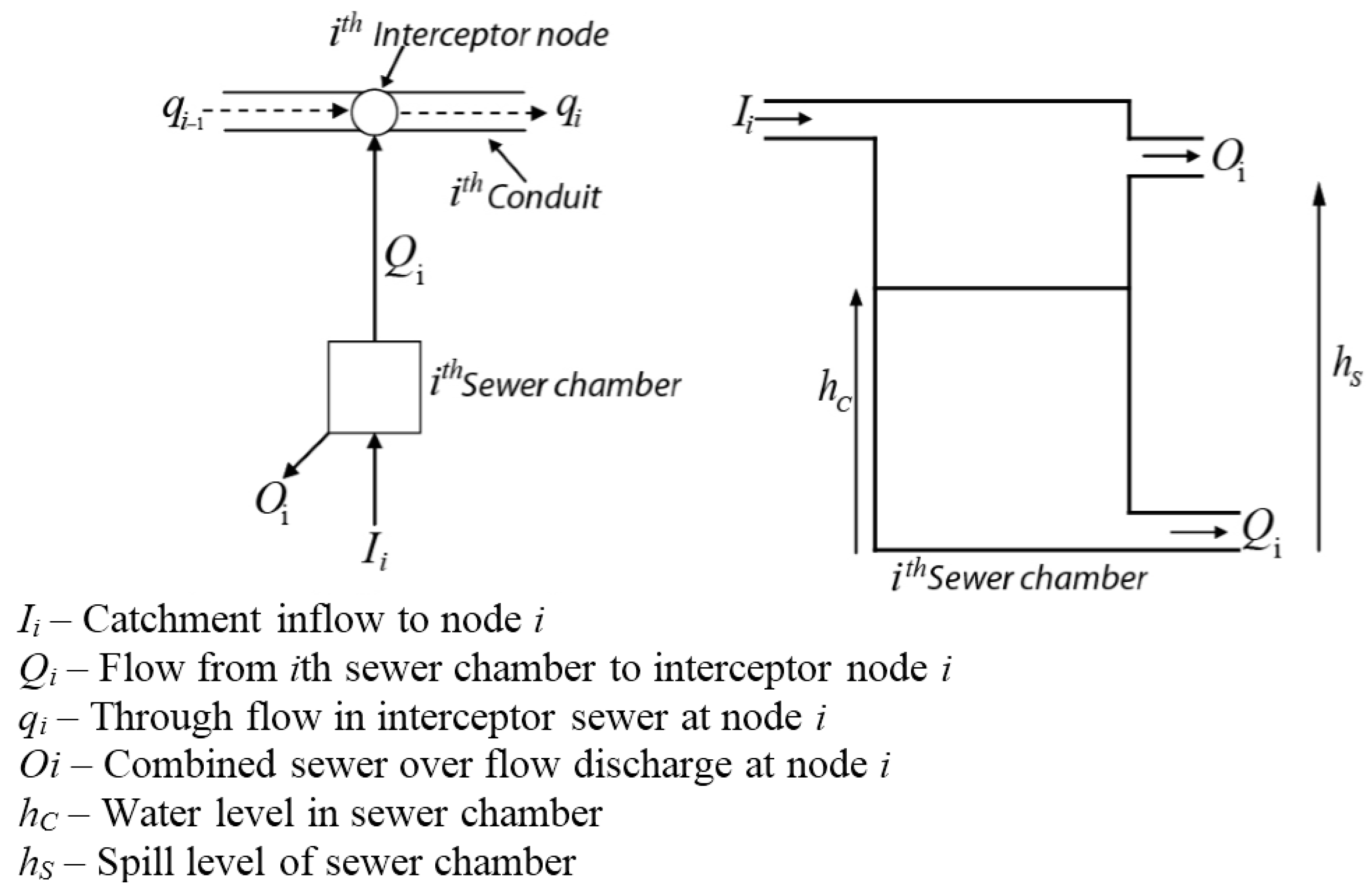
Figure 1 illustrates the schematic diagram of an interceptor sewer system. These schematics were used to develop the multi-objective optimization approach in controlling the urban sewer systems.

Figure 1. Schematic diagram of interceptor sewer system.

Figure 1. Schematic diagram of interceptor sewer system.

Equation (1) gives the formulated first objective function (F₁) for the multi-objective optimization approach. This was developed to minimize the pollution load from CSOs. The effluent quality index (EQI) was used to formulate this pollution load. Concentrations of total suspended solids (TSS), chemical oxygen demand (COD), five-day biochemical oxygen demand (BOD), total Kjeldahl nitrogen (TKN), and nitrates/nitrites (NOX) are integrated to develop this EQI. A detailed explanation of this EQI can be found in Rathnayake and Tanyimboh [5,6,7].

$$Minimize{F}_1={\displaystyle \sum _{i=1}^n{P}_i}$$

(1)

where n and P_i are the number of interceptor nodes or CSO chamber points and the pollution load to the receiving water from the ith CSO chamber, respectively. The second objective function (F₂), given in Equation (2), was formulated to minimize the wastewater treatment cost at downstream wastewater treatment plants.

$$Minimize{F}_2=C_T$$

(2)

where C_T (€/year) is the treatment cost at the treatment plant. The corresponding control settings of the sewer networks are the decision variables of these two objective functions. The C_T is expressed as a function of the wastewater volume flow rate (q_T) to the wastewater treatment plant and given in the following equation (Equation (3)).

$$C_T=\{\begin{array}{lll}& 916.862\times {\left(86400\times q_T\right)}^{0.659}& q_T\le 3\times DWF\\ & 916.862\times {\left(3\times DWF\right)}^{0.659}+\frac{2}{3}\left(1.69\left(q_T-3\times DWF\right)+11376\right),& 6\times DWF\ge q_T\ge 3\times DWF\\ & 916.862\times {\left(3\times DWF\right)}^{0.659}+\frac{2}{3}\left(\left(1.69\times 3\times DWF\right)+11376\right),& q_T>6\times DWF\end{array}$$

(3)

where q_T (m³/s) is the treated wastewater volume flow rate. A detailed explanation on the derivation of this generic cost function is given in Rathnayake and Tanyimboh [5,6,7].

Referring to Figure 1, the following continuity equations can be listed. Equation (4) is for the continuity in the interceptor node, whereas Equations (5) and (6) are the conditional continuity equations for the sewer chamber. These two conditional continuity equations are based on the capacity of the ith sewer chamber.

$$Q_i+q_{i-1}-q_i=0$$

(4)

$$A_C\frac{\text{Δ}{h}_C}{\text{Δ}t}=I_i-Q_i; h_C<h_S$$

(5)

$$A_C\frac{\text{Δ}{h}_C}{\text{Δ}t}=I_i-Q_i-O_i; h_C>h_s$$

(6)

where A_C is the surface area of the CSO chamber. Flows inside the interceptor sewers are constrained. These constraints are inserted in the multi-objective optimization approach. The mathematical formulations for the constraints are given in the following equation (Equation (7)).

$$0\le q_i\le q_{\max ,i}$$

(7)

where q_max,i is the maximum flow rate at the ith conduit. Often, combined sewer networks are constructed with storage tanks. They are to provide additional capacities to the sewer network. Formulations for on-line storage tanks were carried out in this research. More information on these formulations can be found in Rathnayake and Tanyimboh [8]. Furthermore, the above-stated continuity Equations (4)–(6) and constraints (Equation (7)) can handle the spatial and temporal behavior of the inflow. Therefore, the implementation of migration storms can be managed without any disruptions.

3. Solution Technique

U.S. EPA SWMM 5.0 [9] is a powerful hydraulic and water quality simulation model. This software is capable of simulating stormwater runoff and routing processes, including water quality routing. SWMM has been successfully used in many practical design and control problems in both combined and separate sewer systems [10,11]. Gradually varied, unsteady flows inside sewers are routed using the mass conservation and momentum equations, i.e., one-dimensional St. Venant equations. In addition, the sewers are assumed to behave as continuously stirred tank reactors for water quality routing. Mass conservation is used to calculate the concentrations of each water quality parameter leaving the conduits at the end of a time-step. The same principle is applied at the storage nodes.

SWMM 5.0 was linked to Non-dominated Sorting Genetic Algorithm (NSGA II) [12] using the C programming language. NSGA II is a multi-objective optimization module and it has already been successfully applied to many practical optimization problems in various disciplines.

NSGA II is a computationally fast and elitist multi-objective evolutionary algorithm. Briefly, an initial parent population of size N is generated randomly. An offspring population also of size N is then generated from the parent population. This involves binary tournament selection and crossover operations that create two children from two parents. On completion of the crossover, a mutation operator that alters a selection of individuals in the offspring population is applied. Then, the parent and offspring populations are merged to form a population of size 2N. The merged population is then sorted into various levels or fronts of non-domination based on the relevant fitness criteria. Finally, a new population of size N is created by taking the best solutions first, according to the rank order of the respective non-domination levels. If any non-domination level has more solutions than required, then preference is given to solutions in the parts of the solution space that are under-represented. This cycle is repeated until the algorithm convergences and/or the specified termination criteria are reached. At the end of the optimization run, the solutions to the objective functions can be plotted as “Pareto optimal fronts”.

A rectangular orifice was placed at the bottom of each CSO chamber. This orifice was used to control the wastewater flow to the interceptor sewer. The orifice openings are, therefore, the control settings or decision variables of the developed multi-objective optimization approach. These orifice openings were initially generated randomly. Then, a full hydraulic simulation, including water quality routing, was carried out using SWMM 5.0. In order to carry out the hydraulic simulations, runoff hydrographs from migrating storms and their corresponding pollutographs were fed to the respective CSO chambers. Generic pollutographs for total suspended solids (TSS), chemical oxygen demand (COD), biochemical oxygen demand (BOD), nitrates and nitrites (NOX), and total Kjeldahl nitrogen (TKN) were generated based on the previous literature [13,14,15,16,17,18,19]. Hydraulic and water quality results from the simulations were used to calculate the two objective functions (F₁ and F₂).

Continuity equations given in Equations (4)–(6) are automatically satisfied by the hydraulic model, SWMM 5.0. However, the constraints given in Equation (7) are satisfied inside the multi-objective optimization module, NSGA II. Constraints in NSGA II are satisfied by a tournament constraint handling approach [12].

4. Case Study

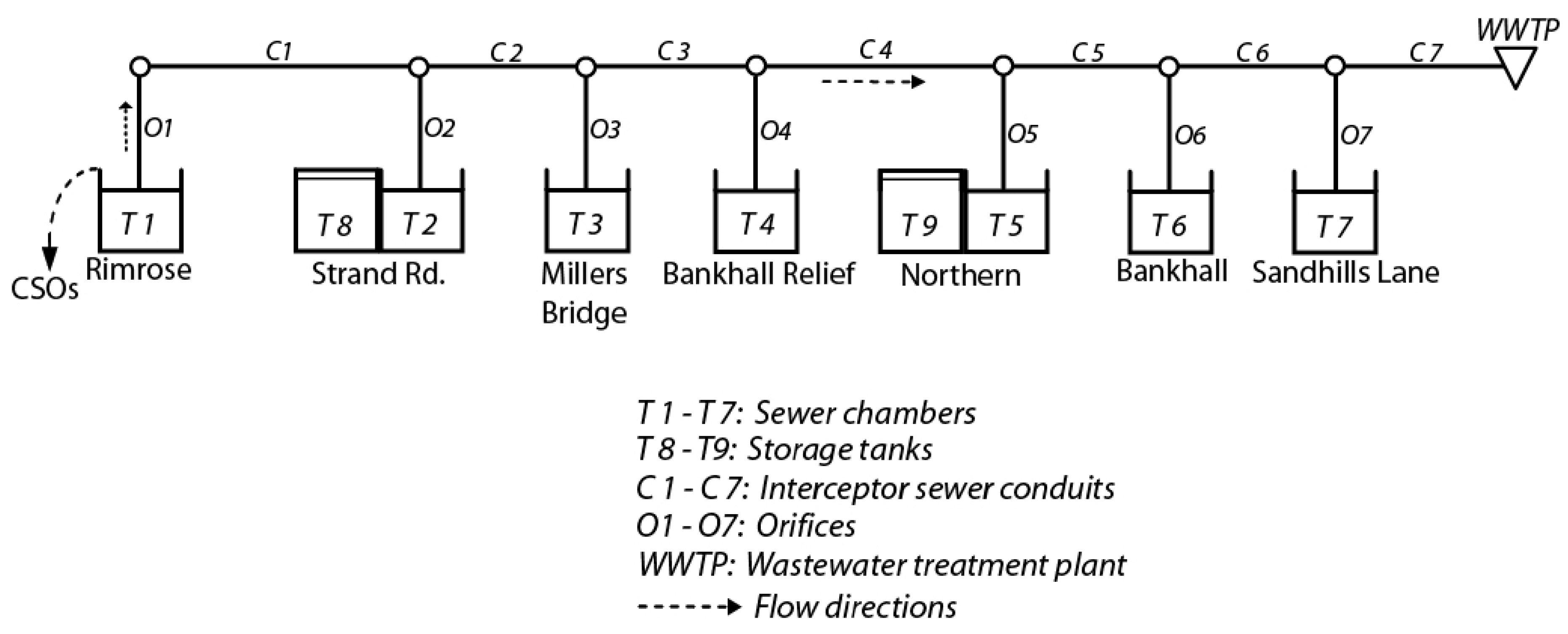
The interceptor sewer system used for this analysis can be seen in Figure 2. The interceptor sewer system found in Thomas [20] was modified for this study.

Figure 2. Interceptor sewer system.

Figure 2. Interceptor sewer system.

Two on-line storage tanks (T8 and T9) were introduced to T2 and T5 CSO chambers. These two on-line storage tanks were controlled inside the hydraulic model. The control rules in SWMM 5.0 were used to control the on-line storage tank. When the wastewater level in the CSO chamber reaches its spill level, the wastewater is transferred to the attached on-line storage tank. However, when the on-line storage tank researches its maximum capacity, this diversion of wastewater from the CSO chamber to the storage tank stops. This avoids having CSOs from any on-line storage tanks. However, when there is less stress on the combined sewer network, the stored wastewater is released back to combined sewer system.

The lengths of the C1–C7 conduits are 895, 740, 460, 15, 719, 19, 710, 350, and 196 m, respectively. More information on the geometric data of the interceptor sewer system is found in Thomas [20] and Rathnayake and Tanyimboh [6]. Flow rates inside the conduits were constrained to 3.26 m³/s in C1–C3 conduits and 7.72 m³/s in C4–C7 conduits.

Average dry weather flows were fed to T1–T7 CSO chambers. Runoff hydrographs for migrating downstream and migrating upstream runoff hydrographs were separately fed to the T1–T7 CSO chambers for two analyses. These migrating storms are illustrated in Figure 3a,b. For simplicity, only a set of generic hydrographs were fed to CSO chambers. The hydrographs presented in Thomas [20] and Rathnayake [6] were modified to represent the migration behavior of the storms. Therefore, Figure 3a presents the migration downstream behavior of the storms whereas Figure 3b shows the migration upstream behavior. However, there is a flexibility in applying the true rainfall data to generate migrating storms in the hydraulic model. Therefore, the model can be applied for any variation of runoff hydrographs.

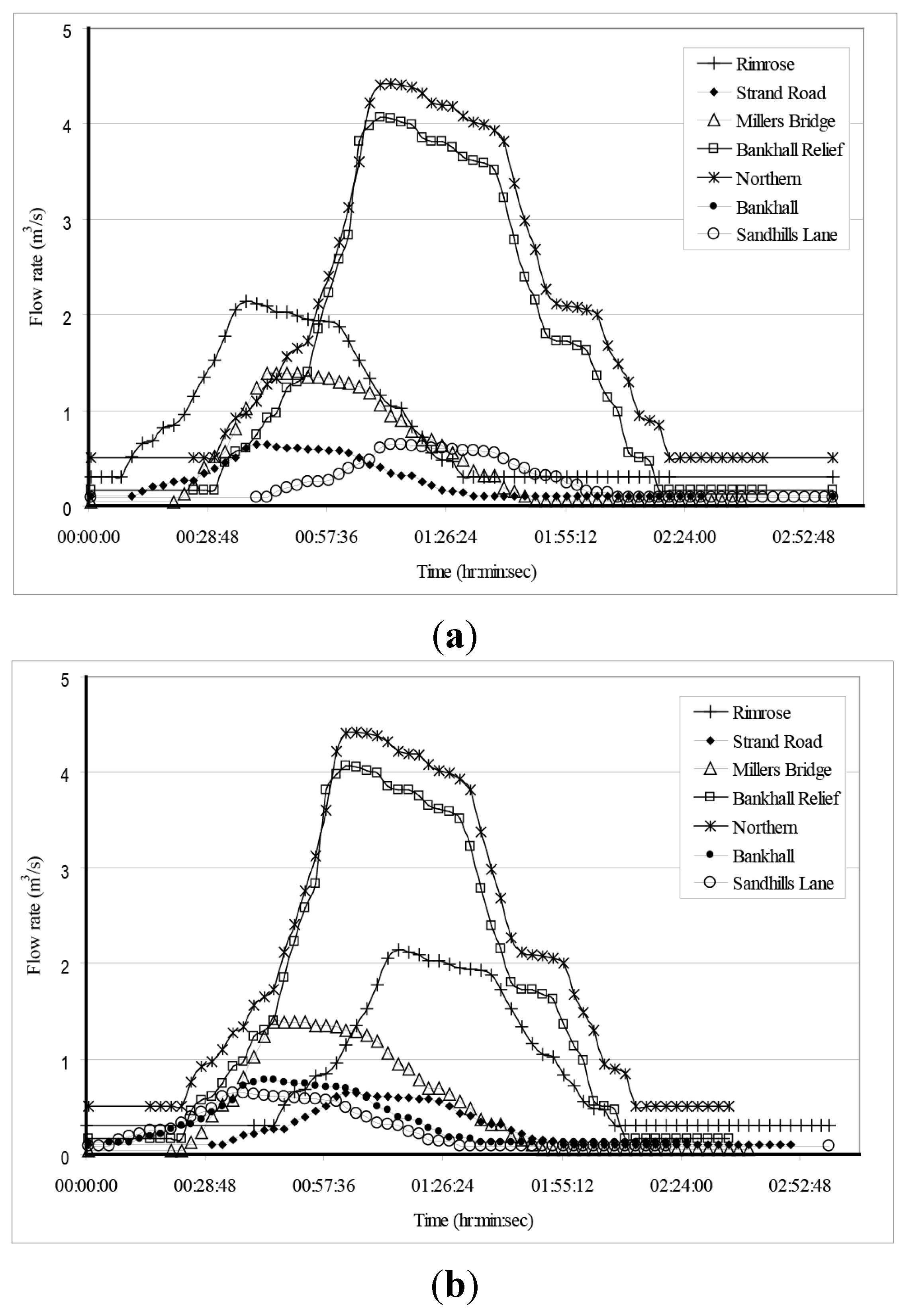
Figure 3. (a) Stormwater runoff hydrograph for migrating downstream storms; (b) Stormwater runoff hydrograph for migrating upstream storms.

Figure 3. (a) Stormwater runoff hydrograph for migrating downstream storms; (b) Stormwater runoff hydrograph for migrating upstream storms.

The peak duration of the hydrographs for the same CSO chamber variation can be clearly seen from Figure 3a,b. The peak flow of the Rimrose catchment to the T1 CSO chamber is around the 30th minute for the migrating downstream storms. However, that of the migrating upstream storms is around the 90th minute. In addition, the peak of the Northern is around the 90th minute in the migrating downstream storms (Figure 3a). Therefore, the two peak flows have a 45 min difference. These features show the migration features of the storms. In addition to the runoff hydrographs, corresponding pollutographs for five different water quality constituents (TSS, COD, BOD, NOX, and TKN) for different land uses (residential, commercial, industrial, agricultural, and mid-urban) were fed to each CSO chamber for the two cases.

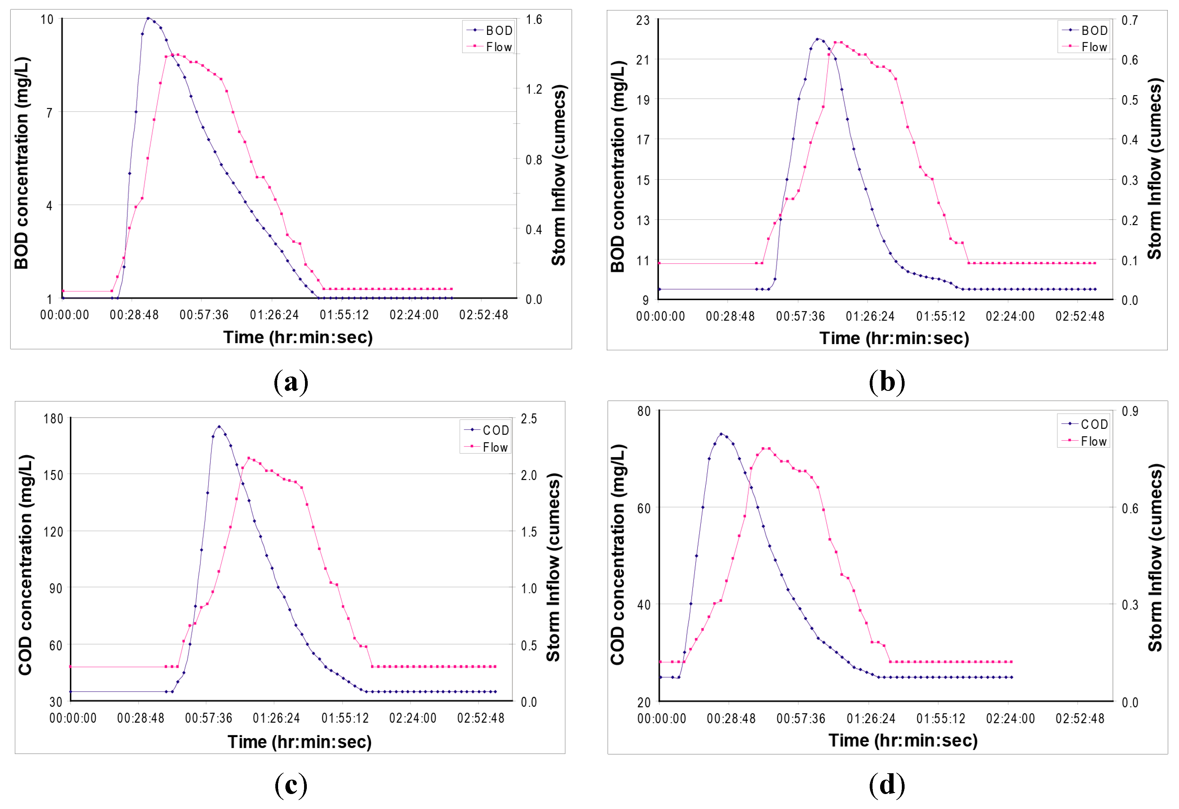
A few pollutographs generated based on previous literature [13,14,15,16,17,18,19] for two different migrating storms can be seen in Figure 4. Figure 4a,b show the BOD pollutographs and the corresponding stormwater runoffs for the Millers Bridge and Sandhills Lane catchments. The concentration levels are different in the two figures due to the different land uses. However, the migrating effects can be clearly visualized in the two figures. The peak of the BOD pollutograph of Figure 4a is roughly at the 30th min of the storm. However, the peak of the BOD pollutograph in Figure 4b has migrated roughly to the 1 h time duration. This is according to the migration of the corresponding stormwater runoff hydrograph. In contrast, Figure 4c,d show the COD pollutographs and the corresponding stormwater runoffs for the Rimrose and Bankhall catchments. The concentration levels are different in the two catchments due to the different land uses. However, the migrating upstream effects can be clearly visualized in the two figures. The peak of the COD pollutograph of the Rimrose catchment is roughly at the 1 h mark of the storm. However, the peak of the COD pollutograph at the Bankhall catchment has migrated roughly to the 30th min of the time duration. This is again according to the migration of the corresponding stormwater runoff hydrograph. It is noted herein that the Bankhall catchment is at the downstream of the combined sewer network.

Figure 4. Pollutographs for migrating storms. (a) BOD pollutograph for Millers Bridge; (b) BOD pollutograph for Sandhills Lane; (c) COD pollutograph for Rimrose; (d) COD pollutograph for Bankhall.

Figure 4. Pollutographs for migrating storms. (a) BOD pollutograph for Millers Bridge; (b) BOD pollutograph for Sandhills Lane; (c) COD pollutograph for Rimrose; (d) COD pollutograph for Bankhall.

Combined sewer network modeling was carried out using the above-stated information. The obtained results from the hydraulic and water quality modeling were input to the NSGA II optimization module. A real-coded NSGA II program was used in this study. The optimization process was done with a population of 100,100 generations for both migrating storm conditions. Many optimization runs with different random seeds were conducted. The routing time-step in SWMM 5.0 was kept at 30 s, and the results were obtained at each 15 min interval for the total duration of the storms. Then, the NSGA II optimization module was run using the obtained results. Each Genetic Algorithm (GA) run took about 42 to 47 min on an Intel^® Core™ i3 desktop personal computer with a 3.40 GHz processor and 4 GB of RAM.

5. Results and Discussion

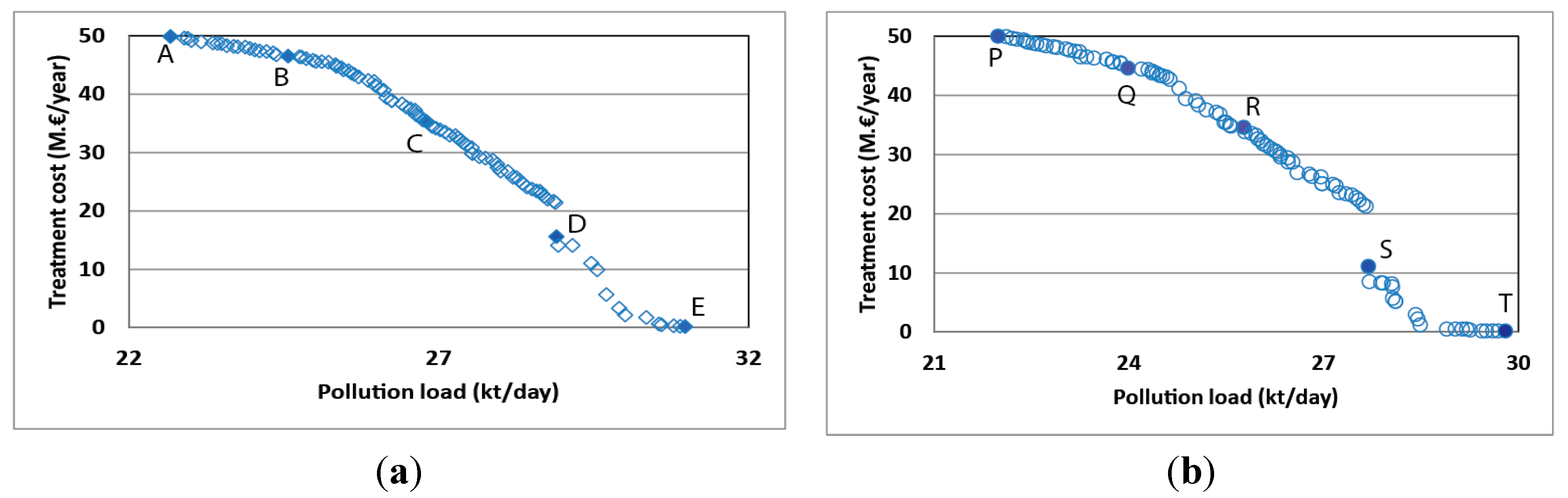
Figure 5a,b show the best Pareto optimal fronts for both storm conditions after 3 h. For the calibration purposes many optimization runs were carried out with different mutation rates. It was found out that the best Pareto optimal fronts can be achieved when the mutation rate is at 0.4 for both migrating downstream and upstream storms. These two Pareto optimal fronts look similar in shape. However, they have different maximums and minimums. For example, the minimum pollution load for the migrating downstream storm condition is 22.67 kt/day whereas that for the migrating upstream storm condition is 21.98 kt/day. The corresponding treatment costs for those mentioned above are 49.87 M.€/year and 49.96 M.€/year, respectively. Therefore, these numerical values clearly show the effects of migrating storms.

Figure 5. Pareto optimial fronts after 3 h runoff. (a) For migrating downstream; (b) For migrating upstream.

Figure 5. Pareto optimial fronts after 3 h runoff. (a) For migrating downstream; (b) For migrating upstream.

Five optimal solutions (A to E and P to T) for each case were selected for further analysis. Solutions A to E are for the migrating downstream storm conditions and solutions P to T are for the migrating upstream storm conditions. Solutions A and P correspond to the minimum pollution loads in each case and solutions E and T give minimum treatment costs in each case. Control settings (orifice openings) were obtained for these 10 optimal solutions. 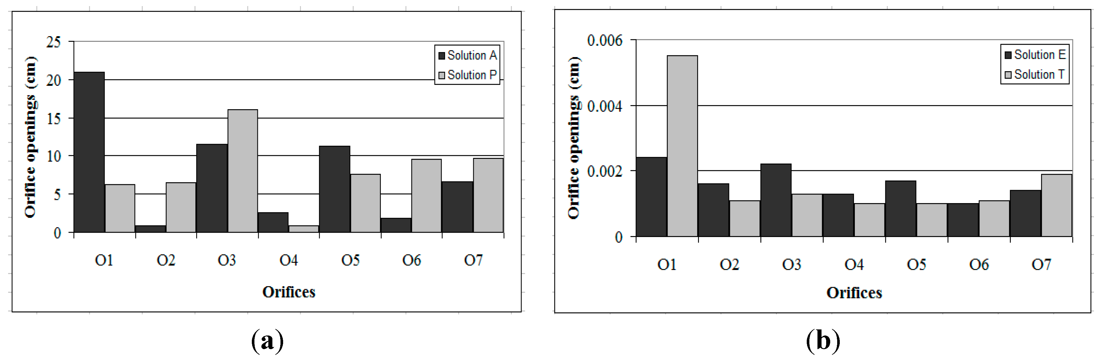Figure 5a,b presents the orifice openings for four optimal solutions.

Figure 6a shows the orifice openings for minimum pollution load solutions, whereas Figure 6b gives the orifice openings for minimum treatment cost solutions. Even though the Pareto optimal fronts (shown in Figure 5a,b) show similar patterns, the corresponding orifice openings are different. For example, the orifice opening for the O1 orifice in the migrating downstream storm condition is about 21 cm; however, that of the migrating upstream storm condition is about 6 cm. This observation can be seen for all other orifices in Figure 6a,b. Therefore, the developed model is capable of handling migrating storms and then producing sound control settings. These obtained orifice openings were used to carry out the hydraulic simulations for each case.

Figure 6. Orifice openings for optimal solutions. (a) Minimum pollution load case; (b) Minimum treatment cost case.

Figure 6. Orifice openings for optimal solutions. (a) Minimum pollution load case; (b) Minimum treatment cost case.

Figure 7a,b present the flow rates inside the interceptor sewers for solution A. As it was stated in the case study section, the flow rates in the conduits were constrained. The maximum allowable flow rate in C1 to C3 conduits was 3.26 m³/s and in C4 to C7 was 7.72 m³/s. Red-color dashed lines in Figure 7a,b graphically represent these maximum allowable flow rates. It can be clearly seen herein that the flow rates in the conduits are lower than the maximum allowed. This shows the developed multi-objective optimization approach produces feasible solutions. In addition, flow rates for the rest of the solutions were checked and the same conclusion can be determined.

Figure 7. Flow rates in interceptor sewers. (a) C1, C2 and C3; (b) C4, C5, C6 and C7.

Figure 7. Flow rates in interceptor sewers. (a) C1, C2 and C3; (b) C4, C5, C6 and C7.

Table 1 presents the wastewater heights in the CSO chambers and storage tanks for solution A. The geometric depths of these tanks from T1 to T9 are 5.42, 6.91, 7.95, 8.04, 8.18, 8.47, 9.26, 6.91, and 8.18 m, respectively. The grey color values shown in the following table are higher than the geometric heights of the corresponding CSO chambers. They represent the CSOs. However, the bold values for the T8 and T9 storage tanks are exactly the same as the geometric depths. They are kept at the maximum possible storage limits and that shows that the role of the storage tanks was well developed for the multi-objective optimization approach. In addition, as it is expected, there are no CSOs for these two storage tanks. This further suggests the robustness of the developed control algorithm.

Table 1. Water heights in CSO chambers and storage tanks.

Time (h:min:s)	Water Height (m)
	T1	T2	T3	T4	T5	T6	T7	T8	T9
0:15:00	5.76	5.55	5.64	7.2	7.71	4.64	3.06	0	1.67
0:30:00	5.99	7.16	8.21	8.22	8.49	8.59	4.96	6.91	8.18
0:45:00	6.14	7.26	8.49	8.5	8.74	8.64	6.29	6.91	8.18
1:00:00	6.1	7.24	8.47	8.89	9.06	8.76	9.42	6.91	8.18
1:15:00	5.87	7.14	8.35	9.04	9.18	8.86	9.56	6.91	8.18
1:30:00	5.64	7.06	8.21	9.04	9.18	8.83	9.54	6.91	8.18
1:45:00	5.61	7.04	8.01	8.88	9.14	8.72	9.46	6.91	8.18
2:00:00	5.61	7.04	7.57	8.69	8.92	8.62	9.34	6.91	8.18
2:15:00	5.61	7.04	7.46	8.35	8.62	8.6	9.2	6.91	8.18
2:30:00	5.61	7.04	7.44	8.22	8.49	8.6	9.09	6.91	8.18
2:45:00	5.61	7.04	7.43	8.22	8.49	8.6	9	6.91	8.18
3:00:00	5.61	7.03	7.43	8.21	8.48	8.59	8.94	6.91	8.18

Table 1. Water heights in CSO chambers and storage tanks.

Time (h:min:s)	Water Height (m)
	T1	T2	T3	T4	T5	T6	T7	T8	T9
0:15:00	5.76	5.55	5.64	7.2	7.71	4.64	3.06	0	1.67
0:30:00	5.99	7.16	8.21	8.22	8.49	8.59	4.96	6.91	8.18
0:45:00	6.14	7.26	8.49	8.5	8.74	8.64	6.29	6.91	8.18
1:00:00	6.1	7.24	8.47	8.89	9.06	8.76	9.42	6.91	8.18
1:15:00	5.87	7.14	8.35	9.04	9.18	8.86	9.56	6.91	8.18
1:30:00	5.64	7.06	8.21	9.04	9.18	8.83	9.54	6.91	8.18
1:45:00	5.61	7.04	8.01	8.88	9.14	8.72	9.46	6.91	8.18
2:00:00	5.61	7.04	7.57	8.69	8.92	8.62	9.34	6.91	8.18
2:15:00	5.61	7.04	7.46	8.35	8.62	8.6	9.2	6.91	8.18
2:30:00	5.61	7.04	7.44	8.22	8.49	8.6	9.09	6.91	8.18
2:45:00	5.61	7.04	7.43	8.22	8.49	8.6	9	6.91	8.18
3:00:00	5.61	7.03	7.43	8.21	8.48	8.59	8.94	6.91	8.18

Table 2 presents the total treated wastewater volumes and total CSO volumes for the four extreme solutions (A, E, P and T). Solution A corresponds to the minimum pollution load approach in migrating downstream storms and shows much higher treated wastewater volumes compared to that of solution E, which corresponds to the minimum treatment cost. A similar observation can be visualized in the migrating upstream storm case. In contrast, total CSO volumes in solutions A and P are lower than those in solutions E and T. Therefore, the optimization algorithm is robust even in volumetric measures.

Table 2. Total treated wastewater and CSOs.

	A	E	P	T
Total treated wastewater volume (m3)	5432.1	12.3	5394.5	11.5
Total CSO volume (m3)	6876.2	7737.3	6682.8	7392.7

Table 2. Total treated wastewater and CSOs.

	A	E	P	T
Total treated wastewater volume (m3)	5432.1	12.3	5394.5	11.5
Total CSO volume (m3)	6876.2	7737.3	6682.8	7392.7

6. Conclusions

Rathnayake and Tanyimboh’s optimal control algorithm was successfully applied for migrating storm conditions. Hydraulic analysis shows that the developed multi-objective optimization control algorithm produces feasible results. In addition, the role of the storage tanks was well placed for the control algorithm. Further research should be carried out in order to apply this optimal control algorithm in real-time controls.