Computations of a Bluff-Body Stabilised Premixed Flames Using ERN Method

Abstract

Combustible carbon-based energy is still prevailing as the world’s leading energy due to its high energy density. However, the oxidation of these hydrocarbons disturbs the natural carbon cycle greatly by increasing greenhouse gases. As emission legislation becomes more rigorous, lean premixed combustion becomes promising because it can reduce nitrogen oxides (NO_x) and Carbon Monoxide (CO) emissions without compromising efficiency. However, utilising lean premixed flames in industrial combustors is not easy because of its thermo-acoustic instabilities associated with pressure fluctuations and the non-linearity in the mean reaction rate. Therefore, reliable predictive combustion models are required to predict emissions with sensible computational costs to use the mode efficiently in designing environmentally friendly combustion systems. Along with the promising methodologies capable of modelling turbulent premixed flames with low computational costs is the ERN-RANS framework. Thus, this study aims to compute a bluff-body stabilised premixed flames close to blow-Off using the ERN-RANS framework. As a result, a satisfactory agreement is reached between the predicted and measured values.

1. Introduction

Climate change is one of the most significant threatening issues of our time. In recent years, an alarmingly increasing trend in the average global temperature has been monitored and reported by international organisations, such as Intergovernmental Panel on Climate Change (IPCC), the European Environmental Agency (EEA), the United Nations Environmental Program (UNEP), the National Aeronautics Space Administration (NASA), and others. At present, combustible carbon-based energy is still prevalent as the world’s prime energy source due to its high energy density [1]. However, in addition to the lack of broad availability, the oxidation of these hydrocarbons substantially unbalances the natural carbon cycle by rising greenhouse gases [1]. Further, burning these fuels cause health, economic, and other related environmental issues, i.e., acid rains, ozone depletion, and atmospheric pollution [1]. For instance, air pollution kills an estimated seven million people annually and damages the ecosystem. The transport and power generation sectors significantly share these harmful effects [2]. Thus, environmental legislation has become more stringent to reduce these adverse effects. The Paris agreement [3] was the latest to enhance the global response to climate change by keeping the global average temperature increase below two degrees Celsius above pre-industrial levels during this century.

Indeed, the growing environmental awareness has resulted in an increasing interest in renewable energy. Still, the share of the production of renewable energy is insignificant [4]. Moreover, combustible fuels are unlikely to be replaced with renewable energy soon (hydro, wind, etc.), explicitly for high energy-density applications, such as aviation, maritime, and power generation sectors.

Recently, lean premixed combustion has become under the spotlight because it can decrease nitrogen oxides (NO_x) emissions without compromising efficiency [5,6,7]. Nevertheless, utilising premixed flames in a lean mode for industrial combustors is not straightforward because of its thermo-acoustic instabilities associated with pressure fluctuations. These oscillations lead to the fluctuation of the fuel–air ratio by changing the inlet flow rates that change in return the combustion rate [5,6]. It is observed that a local extinction might occur if the fuel–air ratio drops significantly [8,9]. Additionally, there is a strong coupling between turbulence, chemical reaction, and diffusion in lean premixed flames [10,11].

Additionally, the reaction rate is a nonlinear function of temperature and species concentration in turbulent combustion. Hence, obtaining an estimate based on the average values is imprecise because of the high fluctuations of the species mass fractions, temperature, and enthalpy over the mean [10,11]. These constraints are a challenge in modelling turbulent lean premixed flames. Therefore, more sophisticated and low-cost numerical models are required to design and develop the next generation of low emissions lean combustion systems.

As discussed in Section 2, the equivalent reaction networks ERN-RANS framework can model turbulent premixed flames with low computational cost. Thus, in this study, the framework [12] is used to compute lean turbulent flame stabilised by a bluff-body [13,14].

This article is constructed as follows. The background and the mathematical formulation of the ERN approach are discussed in the next section, and the test flame is presented in Section 3. The computational details are discussed in Section 4, followed by the results in Section 5. Eventually, the conclusions of this study are summarised in the last section.

2. The Equivalent Reaction Networks (ERN) Method

The ERN approach was formulated in 1953 by [12] and later enhanced by [15]. The framework was used to several combustion problems, such as turbulent premixed flames [16], boilers [15,17,18], swirling flames [19], industrial burners [20,21], and gas turbine combustors [22,23,24]. The main aim of the method is to simplify the turbulent flow behaviour to lower the involved computational cost without reducing the computational accuracy. The ERN algorithm post-process is a fully converged mean flow field obtained using a reduced chemical mechanism. This technique allows simulating combustion problems with complex geometries with reasonable computational costs. The equivalent reactors network zones are constructed using the flow solution mesh based on global criteria. The zones are selected with homogeneous physical and chemical conditions, such as density, temperature, equivalence ratio, and mass fraction. For predicting NO${}_{\mathrm{x}}$ and CO emissions, the stoichiometry and temperature conditions are the best selection as global criteria since they greatly affect NO${}_{\mathrm{x}}$ formation. Based on the selected criteria, the CFD mesh is divided into zones categorised as a perfectly stirred reactor (PSR) or a plug flow reactor (PFR). Suppose the mean axial velocity obtained from the fully converged solution is low. In that case, the region is constructed as a PSR reactor, and if the mean axial velocity is high, the region is constructed as a PFR reactor. The ERN solves the transport equation for each reactor as follows.

$$\frac{d{M}_k}{dt}=M{W}_{k}V{\dot{\omega }}_k+\dot{m_i}\sum _{i=1}^{N_{inlets}}{Y}_k-\dot{m_j}\sum _{j=1}^{N_{outlets}}{Y}_k.$$

(1)

The LHS term in Equation (1) represents the unsteady part in the transport equation. The first term on the RHS represents the mass rate of species k within the control volume. Where V, ${\dot{\omega }}_k$ is the volumetric reaction rate, and $W_k$ is the molecular weight for species k within the control volume. The second and the third terms on the RHS represent the rates of mass flow entering and exiting the reactor, respectively. Where $\dot{m_i}$ and $\dot{m_j}$ are the mass flow rates passing into the reactor from inlet, i, and outlet, j. $Y_k$ is the mass fraction of species k. The energy transport equation is written as

$$\frac{dU}{dt}=\dot{m_j}\sum _{j=1}^{N_{outlets}}{Y}_{k,j}{h}_k-\dot{m_i}\sum _{i=1}^{N_{inlets}}{Y}_{k,i}{h}_k,$$

(2)

where U denotes the internal energy. $h_k$ signifies the absolute enthalpy, which is defined as the sum of the enthalpies of formation, $h_{f,k}^{\circ }$, at a reference temperature, $T_{\mathrm{ref}}$, and sensible enthalpy, $h^s$.

$$h^s=h_{f,k}^{\circ }+{\int }_{T_{ref}}^T{c}_{pk}\left(T\right)dT,$$

(3)

T represents the absolute temperature within the reactor, and $c_{pk}$ is the heat capacity of species k. The PFR reactor simplifies the flow in one direction with no axial mixing. Consequently, the flow is mainly governed only by diffusion and convection. For a control volume over a slice perpendicular to the direction of the flow, the species and energy transport equations can be written as follows.

$$\rho u\frac{d{Y}_k}{dx}={\dot{\omega }}_k{MW}_k$$

(4)

$$\rho u{c}_p\frac{dT}{dx}=\rho u{c}_p\frac{dh}{dx}-\sum _{k=1}^{n_{sp}}{h}_k{\dot{\omega }}_k{MW}_k$$

(5)

u represents the axial velocity in the direction x. $c_p$ denotes the mixture heat capacity, and $n_{sp}$ is the number of species participating in the chemical mechanism. The ERN equations are solved along with the equations for conservation of mass and momentum.

3. Test Flames and Experimental Setup

In the present study, the bluff-body stabilised turbulent premixed flame [13,14,25], illustrated schematically in Figure 1, was selected to validate the RANS-ERN methodology. This flame consists of a lean methane-air mixture with an equivalence ratio of $0.586$ and initial conditions of 294 K and 1 atm. The flame is confined in a square-like combustion chamber with a $79\times 79$ mm cross-section. The flame is stabilised using a conical bluff body shape with a diameter of 44.45 mm. The mean initial velocity and turbulence intensity used in the experiment were 15 m/s and $24\%$, respectively. The species mole fractions and temperature were obtained using a combination of spontaneous Raman scattering, Rayleigh scattering, and laser-induced fluorescence. The measurement errors are expressed in terms of the standard deviation.

The experimental aspects of the combustor inlets are summarised in

Table 1. Combustor characteristics.

V (m/s)	D (mm)	T (K)	P (bar)	I (%)	Re (D)
15	44.45	294	1.0	24.0	43,400

. The experiment measured the turbulence conditions and reactive scalars using Laser Doppler Velocimetry and Rayleigh scattering analysis.

4. Computational Details

The Reynolds Averaged Navier Stokes (RANS) technique was utilised to simulate the flow field solution. In this technique, the mean flow field scalars are obtained by solving the discretised closed-form of the Favre averaged transport equations using the commercial CFD code Fluent [26]. The Favre averaged Navier–Stokes equations are discretised using a second-order finite volume technique and computed using a pressure-based solver coupled with the energy and scalar transport equations. An iterative algorithm is used until all the quantities are converged using pre-set convergence criteria.

The mean reaction rate ${\overline{\dot{\omega }}}_k$ term is the focus of the turbulent combustion modelling due to its nonlinearity. This term is modelled using the Eddy-Dissipation formulation [27] with a single-step chemical reaction. In this formulation, the chemical reaction is faster than mixing the reactants by turbulence; hence, the rate of the chemical reaction is governed by mixing. The time-scale of mixing is represented by the turbulent time-scale, ${\tau }_t$. ${\tau }_t=k/\epsilon$, where k is the turbulent kinetic energy and $\epsilon$ the turbulent dissipation rate. The turbulence is modelled using the k-$\epsilon$ model. The model constant $C_{ϵ1}$ is modified from 1.44 to 1.52 to include the round jet anomaly effects [28].

The computational domain created for this computation spans 1100 mm in the axial direction, x, and 120 mm in the radial direction, r. The CFD mesh retains a total physical cell of 630,000. To be noted that the grid dependency was tested, and the results presented in the following section have shown insignificant grid sensitivity.

The initial and boundary conditions used in these calculations are shown schematically in Figure 1, as reported by [13,14]. The combustor inlet temperature and pressure were 298 K and 1 bar. The flow inlet velocity was 15 m/s. A first-order scheme was selected to discretise momentum and species transport equations. The bluff body and combustor walls were evaluated as no-slip walls with radiation heat transfer. The discrete ordinate radiation model was selected. A SIMPLER approach is used to couple the velocity and pressure fields inside the computational domain.

The converged mean flow, temperature, and mass fractions of the major species participating in the chemical reaction are then post-processed using a set of selection criteria. The selection criteria ensure that the finite-volume cells with homogeneous physical and chemical conditions are grouped. It should be noted that a single or joint set of criteria can be chosen. In this study, the mean temperature is selected to create 30 zones so that cells with identical temperature values are clustered together. The created zones are treated individually as an ideal reactor with a volume equal to the sum of the volumes of all clustered finite-volume cells.

The initial conditions of the ideal reactor are acquired by volume-averaging over the CFD cell values. The mass flow that enters each reactor is calculated via volume-averaging over the fluxes of the cell face. The flux through the reactor likewise maintains the essential connections between neighbouring reactors and thus creates a fully-coupled network. The reactor is modelled as a perfectly stirred reactor (PSR) when the local mean velocity inside the reactor is low and is modelled as a plug flow reactor (PFR) when the local mean velocity is high. A residence time for each reactor is correspondingly defined in the form of $\rho V/\dot{m}$, where $\rho$ is the mixture density, V is the reactor volume and $\dot{m}$ is the mass flow rate entering the reactor. The elaborated GRI 3.0 chemical mechanism [29] is utilised to predict the minor and major species.

The computations of the ERN are conducted using an in-house reactor network research code [16]. The calculation of temperature and species mass fractions are acquired by solving the transport equation for the reactor using the open-source solver CANTERA [30]. The solution obtained from the first reactor of the network is then handed to the neighbouring reactors. The mass flow maintains the interchange between the reactors. Eventually, the solution of the reactor network is obtained iteratively, and convergence is checked based on the temperature evolution of each reactor.

A detailed numerical analysis of the formation of small-scale pollutants requires a complex chemical reaction mechanism in conjunction with Computational Fluid Dynamics (CFD). Typically, the computational cost of these analyses is substantial.

In the ERN method, the tool can combine the CFD mesh cells into a network via a fully automated technique based on pre-set criteria. Hence, the computational cost is very low compared to more complex methods while maintaining reasonable accuracy. Yet, ERN is not a substitute for other robust approaches, such as CMC, PDF, or flamelets.

In this study, The computational cost is a linear function of the number of reactors and the number of iterations for convergence. A single simulation on an Intel(R) Xeon(R) CPU X5450 3.00 GHz processor took about 5 h on the wall clock to produce a completely converged solution.

5. Results and Discussion

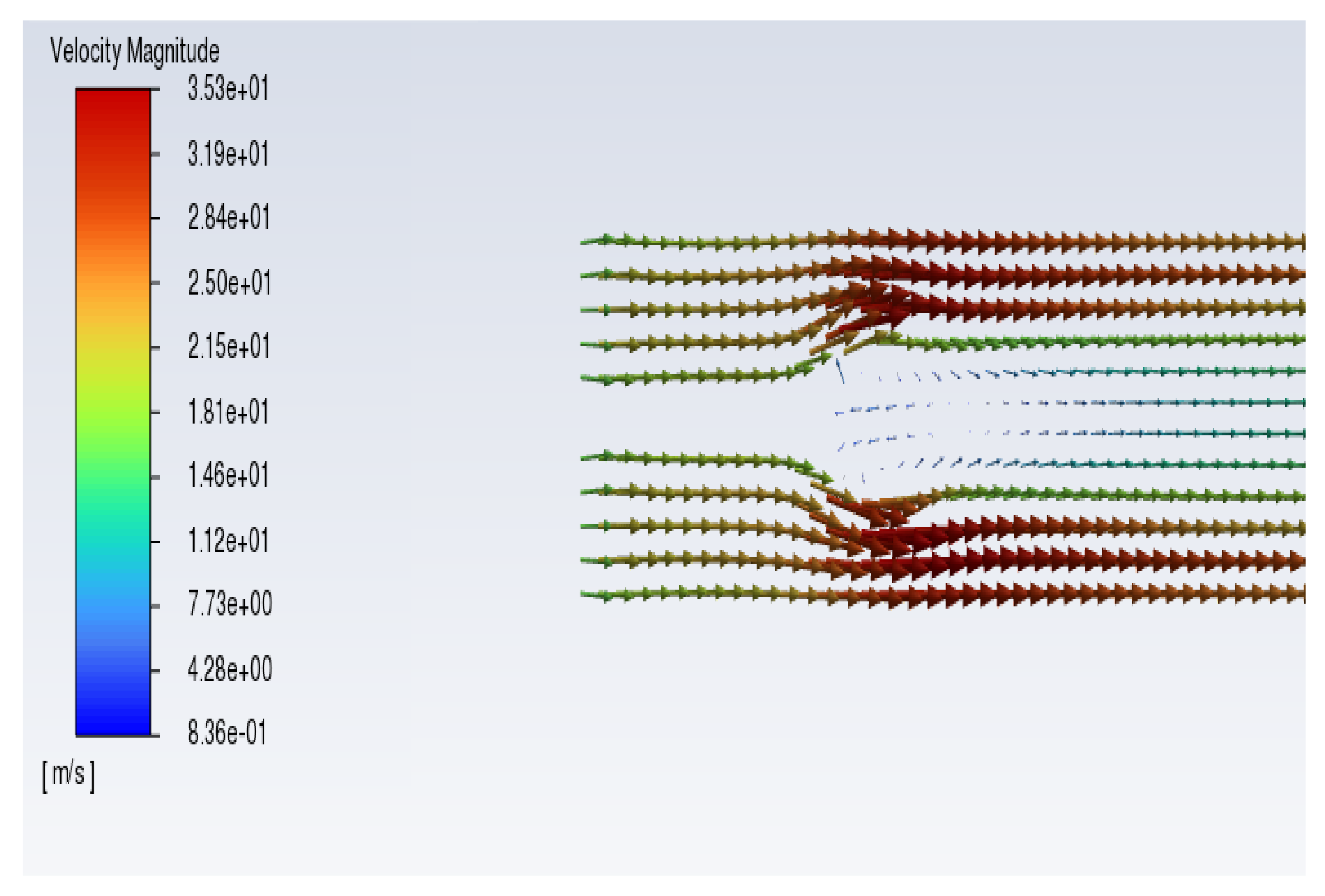
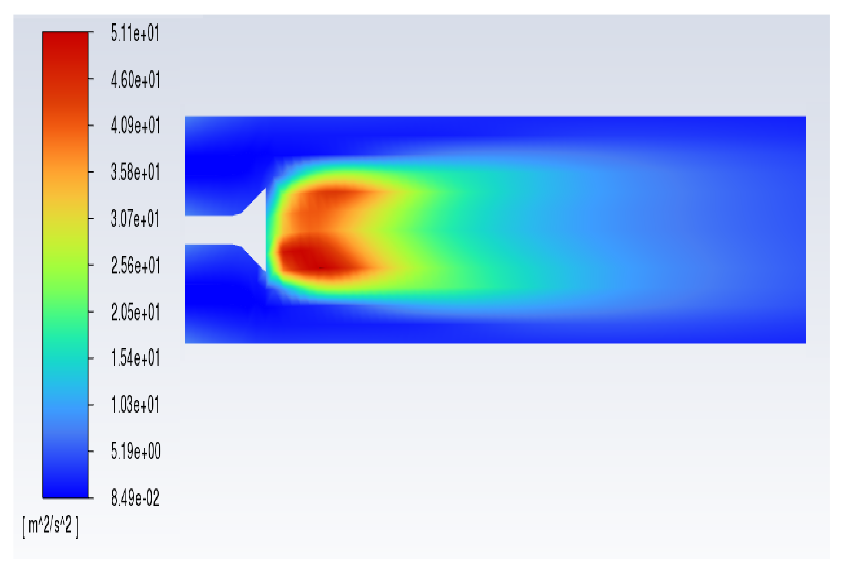
The contours of the mean velocity vectors and turbulent kinetic energy are shown in Figure 2 and Figure 3. The figures show the typical behaviour of bluff-body flames. Nevertheless, the recirculation zone resembles a partially stirred reactor, not a complete stirred reactor which is also indicated in the experimental measurement [13,14].

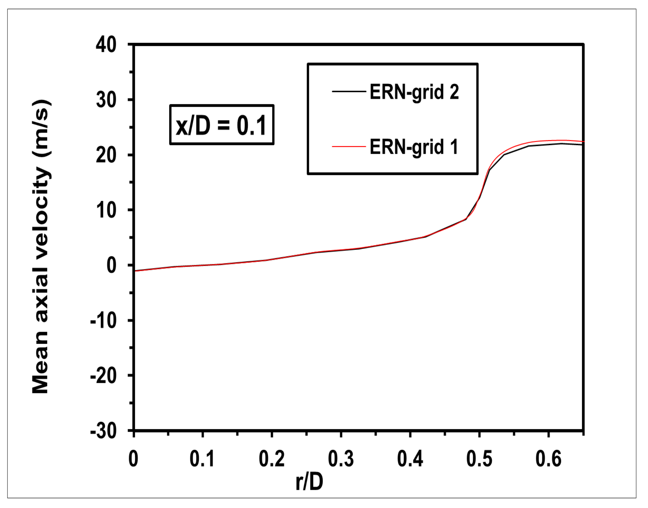
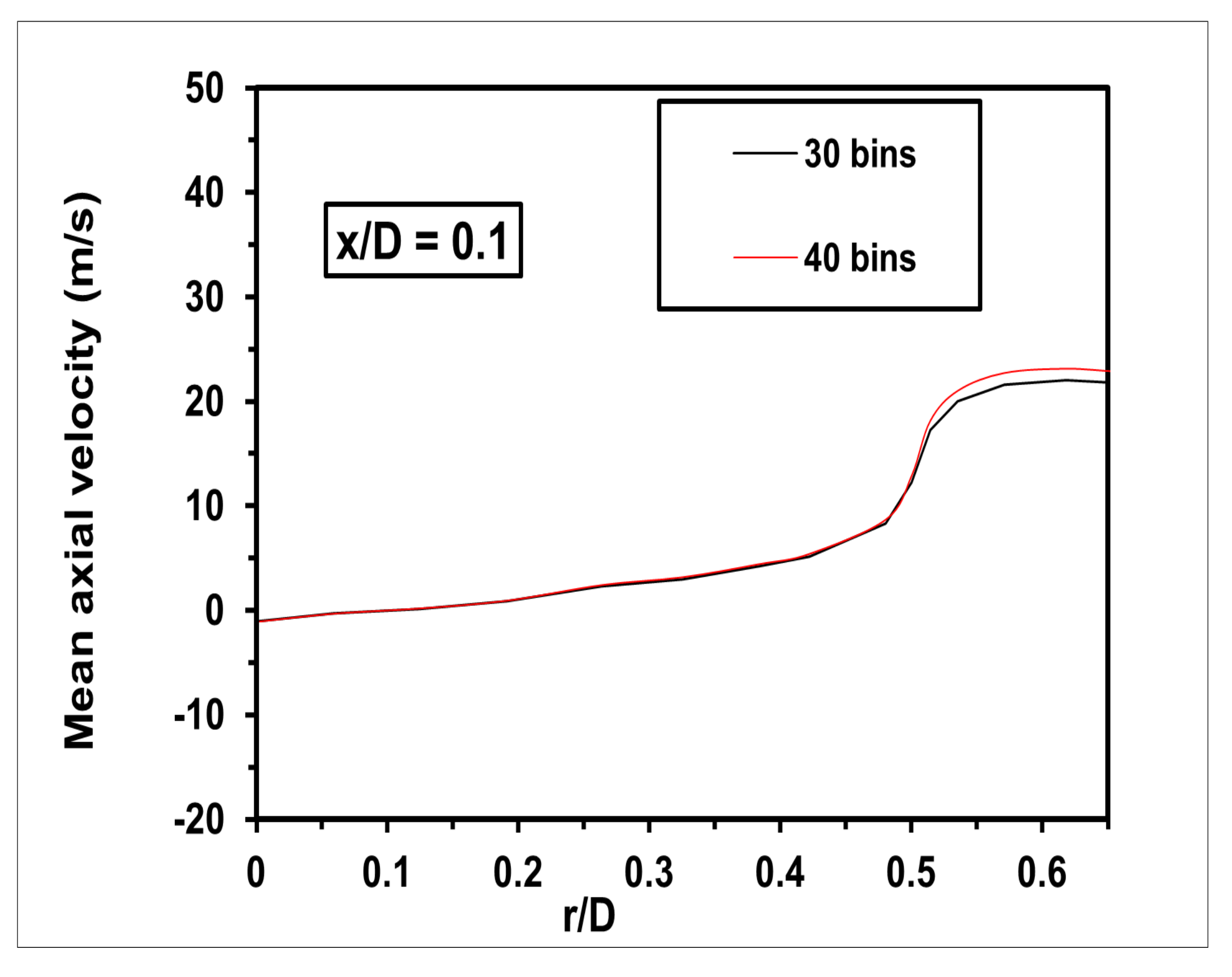
The sensitivity of the solution to the total number of cells is examined. Figure 4 shows the computed mean velocity compared to the experimental measurements at axial locations $x/D$ = 0.1 using two different total numbers of cells, 63,000 and 87,000. As shown, both grids yield comparable results. Furthermore, the sensitivity of the solution obtained from ERN to the selected number of reactors is evaluated utilising other numbers of zones 30 and 40. As illustrated in Figure 5 the mean velocity obtained by 30 zones is equivalent to that obtained using 40 zones. It is noted that a slight discrepancy is seen at $r/D$ ≥ 0.5. Therefore, the following ERN results show insignificant sensitivity to the mean flow grid and the number of ERN bins.

Figure 6, Figure 7, Figure 8, Figure 9, Figure 10 illustrate the the results obtained from the ERN computation compared to the experimental data of Nandula et al. [13,14]. The solid lines illustrate the results obtained from the ERN procedure, and the symbols represent the experimental results. The computed mean quantities are compared at axial locations of $x/D$ equal to 0.1, 0.3, 0.6, 1.0, 1.5, and 2.0.

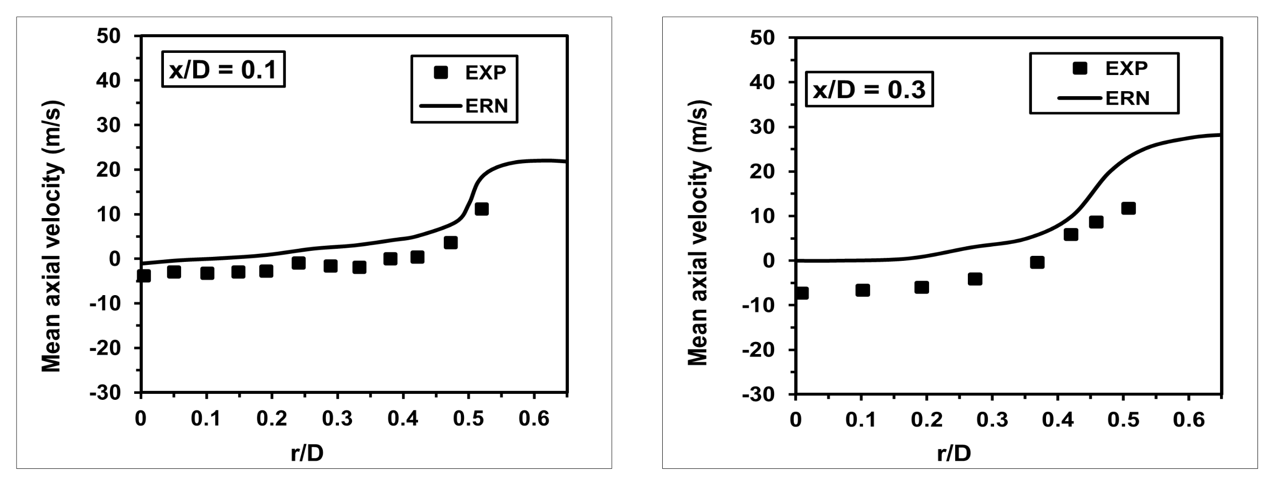
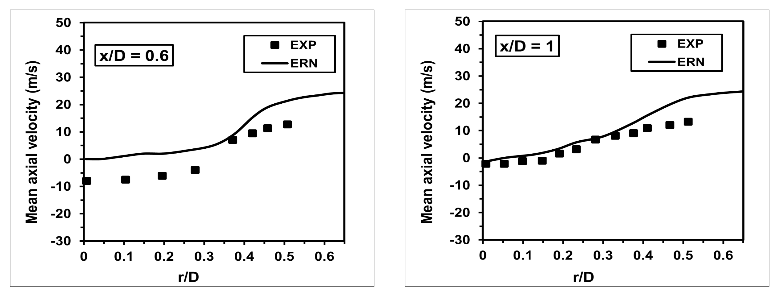
The computed radial profiles of the mean axial velocity are shown in Figure 6. The ERN method captured these profiles accurately at all axial locations in the flame. Additionally, the calculated results are in reasonable agreement with the experimental measurements except at axial location $x/D$ = 0.3 and 0.6, where a noticeable difference is seen. At these locations, the ERN method over-predicts the mean axial velocity. Additionally, unlike the experimental measurements where negative values for the axial velocity at the centreline were seen, the ERN method produced positive values at these locations. It should be noted that the mean flow field solution required by the ERN method is obtained using the standard k-$\epsilon$ turbulence model, and, hence, it is worth examining the sensitivity of flow field calculations toward different turbulence models.

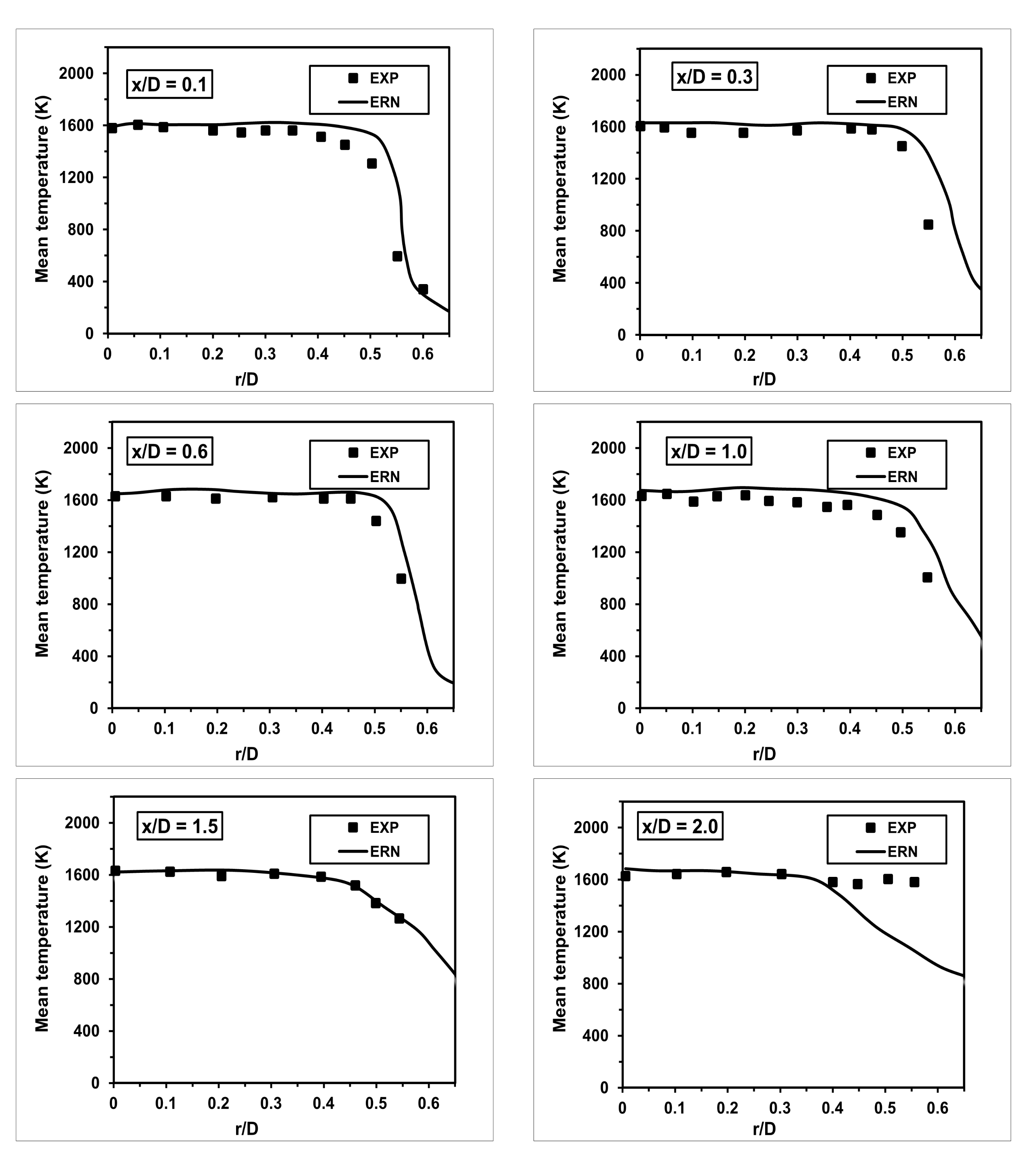
Regarding the mean temperature, the agreement with the experimental data was excellent at almost all axial locations. Furthermore, the method managed to predict the peak temperature at the centerline. However, at the axial location far from the inlet, specifically at axial location $x/D=2.0$, the computed results deviate from experimental measurements at radial locations $r/D>$ 0.4.

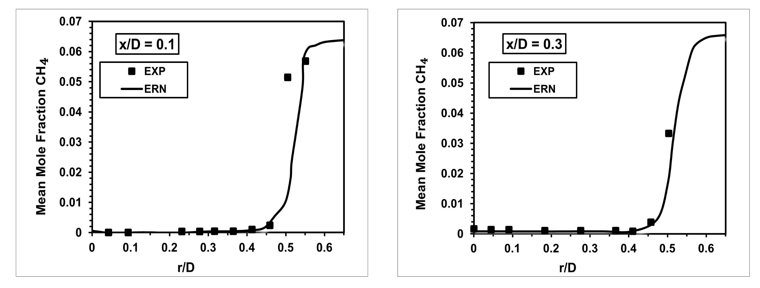
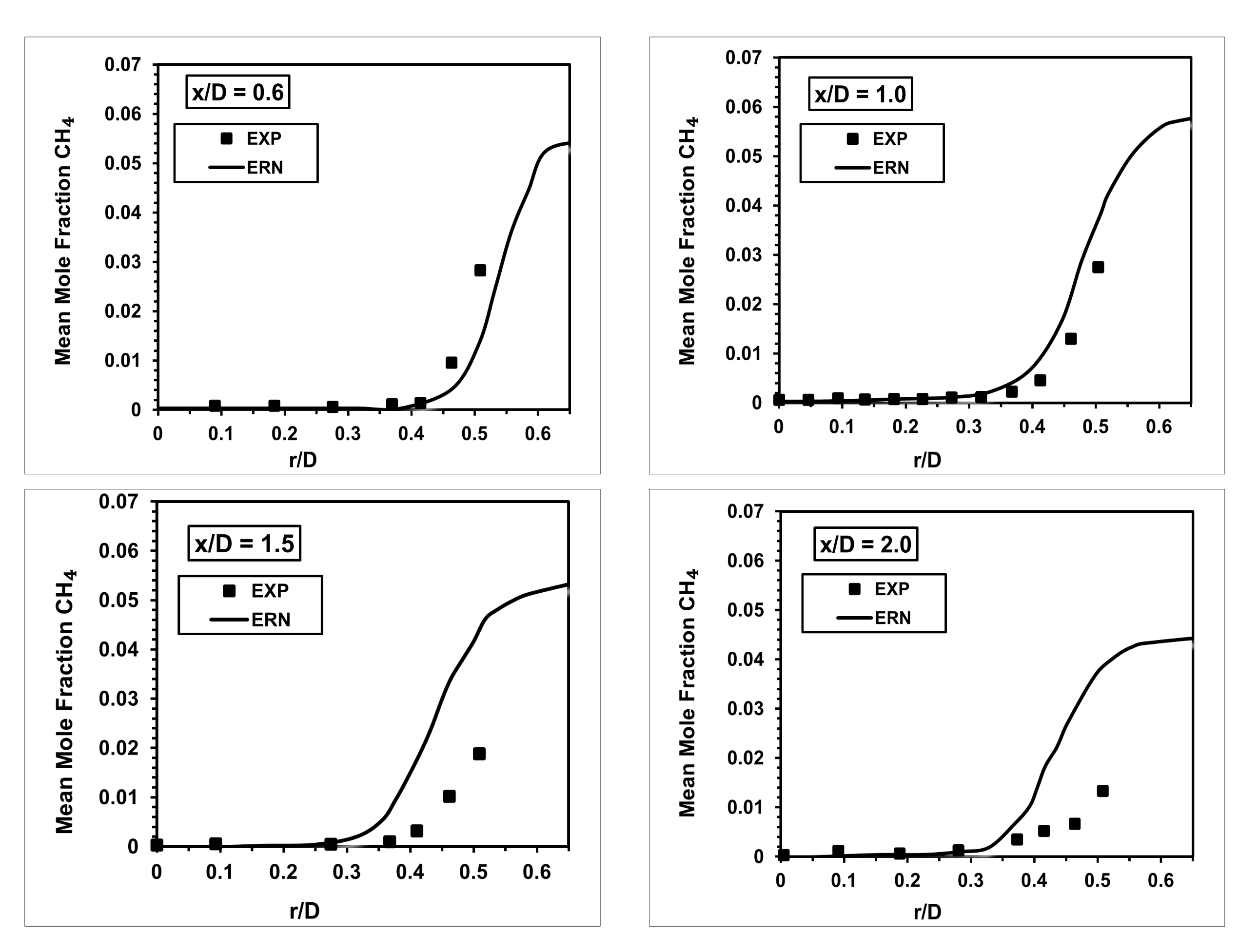
The computed mean mole fraction of CH${}_4$ is compared to the experimental measurements in Figure 8. The figure shows that the agreement between numerical calculations and experiment is less except upstream at axial location $x/D=0.1$, where the ERN managed to mimic the experimental results with minimal error. However, in spite of that, the method was able to predict the radial profiles up to $r/D$ ≤ 0.5 for axial locations $x/D=$ 0.3, 0.6, and 1.0. For unknown reasons at $r/D$ ≥ 0.5, the values of the mean CH${}_4$ are greater than the one reported in the experiment. However, the experiment does not provide more data on these locations to verify the concern.

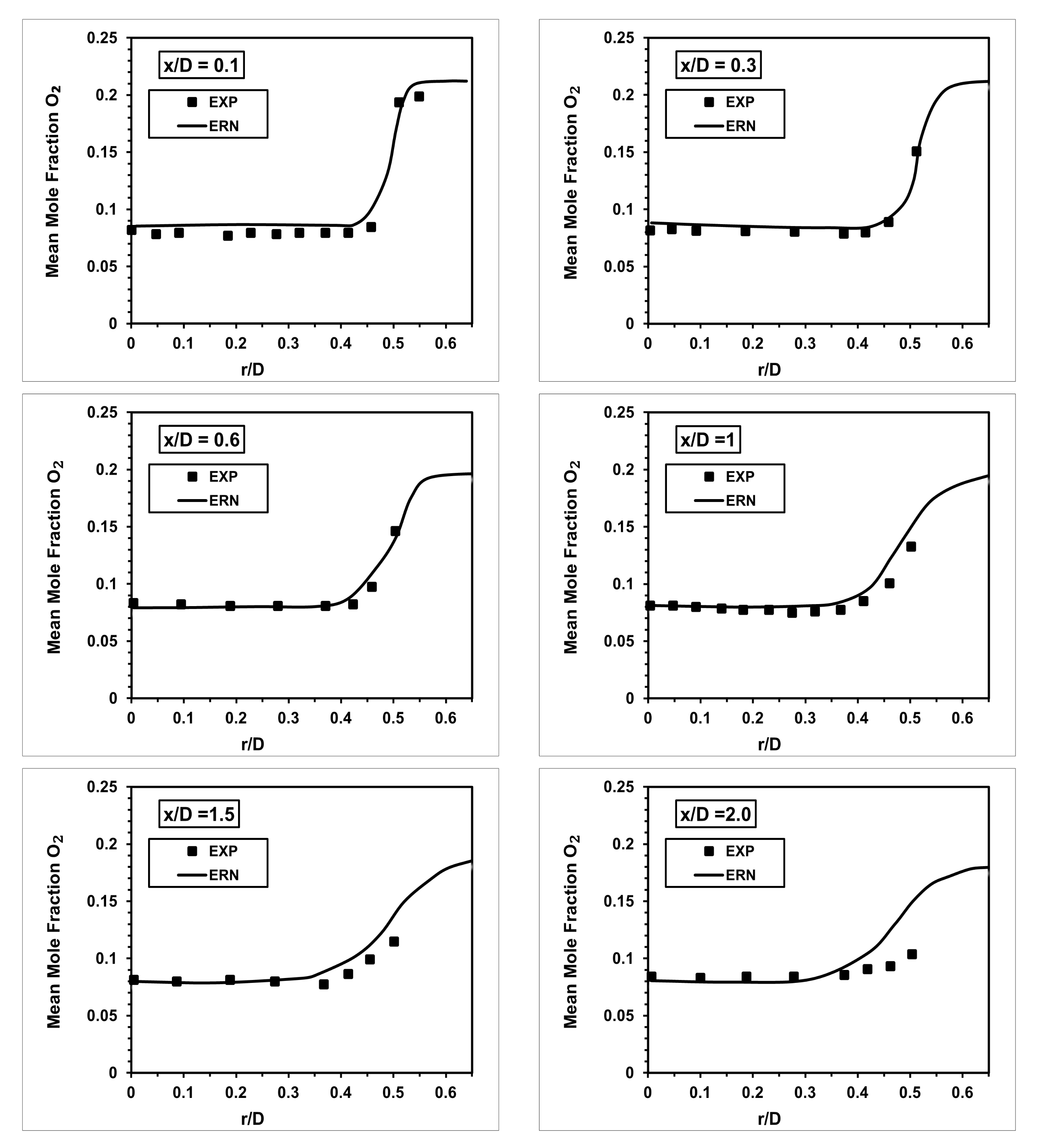
The computed mean mole fraction of CO${}_2$ and O${}_2$ are shown in the Figure 9 and Figure 10. Almost the same argument applies to both, where the computed results reasonably resemble experimental measurements at axial locations $x/D=0.1,0.3,0.6$, and $1.0$. The deviation beyond $x/D=1.0$ is likely due to the selected turbulence model. As for the computed mean CO as shown in Figure 11, the model over predicts the experimental values specifically at location $r/D$ ≥ 0.3. These discrepancies can be attributed to the experimental error or the turbulence model and require further investigation.

6. Conclusions

Lean premixed combustion is a promising strategy because it can decrease nitrogen oxide (NO_x) emissions without compromising efficiency. However, modelling lean premixed flames is challenging because it is notoriously prone to combustion instabilities associated with pressure fluctuations and the non-linearity in the mean reaction rate. In this work, the RANS-ERN approach is used to compute a lean premixed methane–air mixture with an equivalence ratio of $0.586$ at (294 K, 1 atm). The main principle of the method is to reduce the computational cost by post-processing a simple combustion model, such as the Eddy-Dissipation Model with a single-step chemical mechanism and k-$\epsilon$ turbulence model. The converged flow was then post-processed using a set of selection criteria. In this study, the mean temperature is selected to construct 30 ERN zones so that cells with similar temperature values are clustered together. The created zones are treated individually as an ideal reactor with a volume equal to the sum of the volumes of all clustered finite-volume cells. The obtained results, such as mean velocity, temperature and major species mole fractions, are compared to the experimental measurements.