Applied Process Simulation-Driven Oil and Gas Separation Plant Optimization Using Surrogate Modeling and Evolutionary Algorithms


Ramboll Energy, Field Development, Studies & FEED, Bavnehøjvej 5, DK-6700 Esbjerg, Denmark
ChemEngineering 2020, 4(1), 11; https://doi.org/10.3390/chemengineering4010011
Submission received: 30 June 2019
/
Revised: 9 December 2019
/
Accepted: 3 February 2020
/
Published: 6 February 2020
Abstract
:In this article, the optimization of a realistic oil and gas separation plant has been studied. Using Latin Hypercube Sampling (LHS) and rigorous process simulations, surrogate models using Kriging have been established for selected model responses. The surrogate models are used in combination with an evolutionary algorithm for optimizing the operating profit, mainly by maximizing the recoverable oil production. A total of 10 variables representing pressure and temperature at various key places in the separation plant are optimized to maximize the operational profit. The optimization is bounded in the variables and a constraint function is included to ensure that the optimal solution allows export of oil with a Reid Vapor Pressure (RVP) < 12 psia. The main finding is that, while a high pressure is preferred in the first separation stage, apparently a unique optimal setting for the pressure in downstream separators does not appear to exist. In the second stage separator, apparently different, yet more or less equally optimal, settings are revealed. In the third and final separation stage a correlation between the separator pressure and the applied inlet temperature exists, where different combinations of pressure and temperature yields equally optimal results.
1. Introduction
Separation of hydrocarbon reservoir fluids into oil, gas, and water prior to further transport and downstream processing and refining is performed in surface facilities where the multiphase fluids are passed through a number of separators, in which the pressure is gradually decreased to a level where the final oil product is stabilized to a certain degree. This is normally specified as a maximum allowed True Vapor Pressure (TVP) or Reid Vapor Pressure (RVP) value. The surface separation ensures that transportation via pipeline can commence with the crude in the liquid single phase state, without flashing. Further, when reaching the downstream refining facilities, the vapor losses are minimized. Some flashing will occur, and this may provide fuel gas for the refining facilities. However, excessive flashing will occur, if the crude has not been properly stabilized upstream and eventually this may lead to increased flaring, to the harm of the environment.
Depending on a number of parameters such as reservoir fluid inlet pressure, ease of separation due to fluid properties such as density, viscosity etc. and surface facilities space constraints—often experienced on off-shore facilities—the number of separation stages is normally set between 2 to 4 [1]. The first stage pressure is normally set as high as possible without limiting the flow from the reservoir due to back pressure. This minimizes the power requirements for compressing the flash gas for export. The final separation stage pressure is normally set low enough to meet TVP/RVP specifications, or set at stock tank conditions. The intermediate stage pressure(s) are then set in-between, often with consideration to the gas compression system specification and performance.
The challenge is to specify the operating conditions for the separation train which maximizes the profit, which is normally dominated by the export quantity of crude oil [1]. Having a relatively high pressure up to the final separation stage will result in a high quantity of methane (C1)/ethane (C2) being dissolved. These light components flash off in the final separation stage, also attracting some of the valuable middle propane (C3)–pentanes (C5) components. On the other hand, if pressure is too low, the C1–C2 is already flashed off before the final separation stage, but when doing so, some of the C3–C5 may have been lost as well [2]. From this notion, it seems as though setting the pressure just right will preserve as much of the middle components in the crude, while the content of C1 and C2 is low enough when the crude leaves the final separation stage to meet the crude export specifications in terms of RVP/TVP. Besides maximizing the crude production, operating conditions may be optimized in order to reduce the Capital Expenditure (CAPEX), in case of a new design, or to stay within the design capacity of the existing equipment, in case of a plant already in operation.
The complexity in terms of process plant configuration and number of controllable variables is increased with a compression system on top of the separation train. The compression system is responsible for collecting and pressurizing the gas liberated in each of the separation stages, usually a compressor for each stage. The gas pressure is increased enough to allow commingling with the gas liberated in the previous/upstream separation stage. The gas from the first separation stage commingled with gas from all the downstream stages may or may not need further compression. This depends on the operating pressure of the first stage separator, the requirements for gas export pressure, etc. For each compressor the gas is often cooled and any liquid condensed is collected. These condensate streams from compressor suction scrubbers are normally routed back into the separation train.
The selection of separator pressure for optimum stabilized crude production has been the subject of numerous studies. Campbell and Whinery [3] developed a correlation for the optimal second stage pressure in a three stage separation train with the relative molecular weight of the hydrocarbon mixture and a correlating parameter given as a function of C1–C3 content and molecular weight. In a more recent study, Al-Jawad and Hassan [4,5] developed correlations for separation trains with 2–5 stages, and the correlations provide optimal separator pressure for all separators, except the final stage. The required inputs are separator temperatures, methane and impurity content, and upstream separator pressures. Ling et al. [6] investigated the optimum separator pressures assuming constant temperature and well fluid composition for two, three, and four stage separation by successive optimization from the first to last separation stage. Bahadori et al. [7] also made an optimization of separator pressure for a four stage separation train using a commercial process simulator for the flash calculations. Unfortunately, details on the optimization procedure was not provided. Al-Farhan and Ayala [8] trained an Artificial Neural Network (ANN) for a three stage separation train in order to predict optimal second stage separator pressure. First stage pressure as well as fluid composition was varied, providing a exhaustive number of data sets.
Some recent studies employ optimization methods by coupling a commercial process simulator to an optimization routine. Ghaedi et al. [2] coupled a genetic algorithm with a commercial process simulator in order to optimize the crude oil production in a four stage separation train for both a crude oil and a gas condensate well stream, respectively. By optimizing the pressure in the first three separators, it was found that the oil production could be increased by approximately 2% and 8%, for crude and gas condensate, respectively. Motie et al. [9] made a comprehensive study investigating the optimum separator pressure in a multistage separation train, studying the effect of the number of stages, both in terms of operating conditions, but also in terms of an NPV analysis in order to investigate to which extent the added cost of additional equipment for additional separation stages can be justified. The optimization of separator pressures was carried out by means of a genetic algorithm.
Common for [2,3,4,5,6,7,8,9] is the lack of a compression system providing condensate recycle streams i.e., these studies assume a simple straight-through process with the number of controllable variables normally not exceeding 2 to 5.
Kim et al. [1] used a commercial process simulator coupled to an evolutionary algorithm (CMA-ES) in order to optimize separator pressure in both three and four stage separation both with and without condensate recycle streams from the compression system included. When the condensate recycles from the compression system are included, a total of 10 variables are adjusted. The optimization is constrained by a maximum allowed RVP and the objective function is a profit function being maximized.
Andreasen et al. [10] studied a complete oil and gas separation plant with three separation stages, a compression system, as well as hydrocarbon dew point control (cold process) including condensate recycles. Process optimization in terms of minimizing gas compression system power consumption was conducted using constrained optimization using the SLSQP algorithm. Optimization was done on a surrogate model derived by multiple linear regression developed using a commercial process simulator, Design and Analysis of Computer Experiments (DACE) and response surface methodology.
In this paper, optimal operating conditions are investigated for a realistic and complex oil and gas separation plant with: multiple separation stages, a compression system for compressing the flash gas from all separators including condensate recycles, and a cold process for export gas hydrocarbon dew point control. By representing the separation plant with a process simulation model, the means to achieve optimal operating conditions i.e., maximizing the profit, is investigated. An elaborate study taking the full plant complexity into account when studying not just optimal separation stage pressures, but plant-wide operating conditions in general, will contribute to the state-of-art technology.
2. Methodology
2.1. System Description
The process flow sheet forming the basis for the studies presented in the present paper is depicted in Figure 1. In the following, the process configuration is elaborated. The well fluid is routed via an inlet heat exchanger, 20-HA-01, to the first stage separator, 20-VA-01, in which oil and gas is separated. The oil is routed via a level control valve and inter-stage heater, 20-HA-02, to the second stage separator, 20-VA-02, operated at a lower pressure. In the separator, oil and gas is separated. The oil is routed via a level control valve and the second inter-stage heater, 20-HA-03, to the third (final) separation stage. The separated oil is routed via a crude cooler, 21-HA-01, to the oil export pump, 21-PA-01.
The flash gas from the third stage separator is routed via the LP (3rd stage) compressor suction cooler, 23-HA-03, to the LP compressor suction scrubber, 23-VG-03. Condensed liquid is pumped by the condensate recycle pump, 23-PA-01, and discharged upstream to the third stage separator and second inter-stage heater. The gas from the scrubber is compressed in the LP compressor, 23-KA-03, and the compressed gas is commingled with the flash gas from the second stage separator, 20-VA-02. The commingled gas is cooled in the MP compressor suction cooler, 23-HA-02, and routed to the MP (2nd stage) compressor suction scrubber, 23-VG-02, where condensed liquid is knocked out and commingled with the liquid from the second stage separator as well as condensate from the condensate recycle pump, 23-PA-01. The gas from the MP compressor suction scrubber is compressed in the MP compressor, 23-KA-02, and commingled with the gas from the first stage separator, 20-VA-01. The commingled gas is further commingled with condensate from the LT knock-out drum, 25-VG-01 (part of the dew point control unit), before being cooled in the HP (1st stage) compressor suction cooler, 23-HA-01, and with subsequent condensate knock-out in the HP compressor suction scrubber, 23-VG-01.
The compressed gas is cooled in the dehydration inlet cooler, 24-HA-01, and condensed liquid is collected in the dehydration inlet scrubber, 24-VG-01. The gas is dehydrated in the glycol contactor, 24-VB-01. Dry gas is used as fuel gas. The dehydrated gas is further processed in the dew point control unit, consisting of heat exchangers 25-HA-01 and 25-HA-02. The former is used for heat recovery with cross exchange with the dew point controlled dry gas, and 25-HA-02 is for simplicity assumed to be cooled by mechanical refrigeration. Typical alternatives employed especially in off-shore oil and gas facilities includes both Joule–Thomson (J-T) cooling using a simple valve, and sometimes a turbo-expander/re-compressor on a common shaft for deeper Natural Gas Liquid (NGL) recovery, and severe hydrocarbon dew point suppression. In the present study, a refrigeration process is assumed. The cooled gas is routed to the LT knock-out drum, 25-VG-01, where condensed liquid is collected and routed to the HP compressor suction cooler. The cold dew point controlled gas is used for cooling of the water dry gas in the heat exchanger 25-HA-01 before being further pressurized in the export compressor 27-KA-01. Before leaving the facilities, the gas is cooled in the export gas cooler, 27-HA-01.
2.2. Fluid Description
The reservoir fluid investigated in the present study has been adapted from [7] and the composition and fluid characterization in terms of hypotheticals/pseudo-components are shown in Table 1.
The phase envelope of the fluid is depicted in Figure 2. The cricondentherm is 469 C, and the cricondenbar is 289.1 barg. The GOR is 200 Sm/Sm.
2.3. Simulation Setup
All process simulations were carried out using the Aspen HYSYS ver. 10 (AspenTech, Bedford, MA, USA) process simulator. The process flow diagram shown in Figure 1 is modeled in the process simulation flow sheet. The fluid was described using the Peng–Robinson equation of state [11], and liquid density was estimated using the Corresponding States Liquid Density (COSTALD) method [12]. The process simulation file is included in the Supplementary Materials.
A common simulation case was setup with a standard setting of parameters as displayed in Table 2. Further, assumed bounds for the variables are also included and shown in the table.
Along with parameter settings, key process simulation output is also included i.e., calculated operating profit, oil export rate, power, and oil export RVP. In the following, when referring to RVP, it is implicitly assumed that it is at a temperature of 37.8 C. The parameter settings were set with the following considerations in mind: The 1st stage separator (20-VA-01) pressure was set as high as possible in order to reduce compression cost (assuming that the flowing wellhead pressure was higher), the 3rd stage separator (20-VA-03) pressure was set to 1.5 barg (arbitrary), the 2nd stage separator (20-VA-02) was set in order to have an equal pressure ratio between 1st to 2nd stage and 2nd to 3rd. The pressure after the HP/1st stage compressor (23-KA-01) was set to 90 barg, in order to provide a reasonable high pressure ratio. The remaining parameters were arbitrarily set. The bounds applied to the variables in the present study are based on offshore facilities and practical considerations for e.g., cooling a medium system (assuming North Sea conditions). For such facilities, the lower cooling medium temperature is limited by the ambient seawater temperature.
An internal calculation was setup in the process simulation, whereby the total power was summarized, taking both direct process consumers into account as well as indirect consumers (not modeled in the flow sheet) such as cooling medium pumps, sea water lift pumps for cooling medium cooling and heating medium pumps (if required). In order to calculate the required cooling medium flow and related pumping power, a Cooling Medium (CM) duty balance was made by summing up all the individual cooling duties. Further, a CM density of 1000 kg/m, a temperature rise T = 20 C, and a specific heat capacity of 3.8 kJ/kg was assumed. A similar approach was made for the HM balance, but with a slightly higher heat capacity of 3.9 kJ/kg. The exchangers 20-HA-01 and 20-HA-03 can function as either coolers or heaters, depending on the specified variables.
For seawater, the assumed heat capacity was 4.0 kJ/kg and T = 10 C was assumed and the duty was equated to the CM duty. Utility pumping power was based on a pump efficiency of 75% and a pump head of 55 m for CM and HM pumps and 100 m for SW lift pumps. The power required for refrigerant compression was assumed to be 25% of the refrigeration cooling duty. This corresponds roughly to an evaporator temperature of −5 C and a condenser temperature of 30–35 C using propane in a single stage refrigeration process [13].
Based on the calculated total power consumption of main process and utility consumers, the corresponding amount of fuel gas needed for fueling a gas turbine power generator was calculated based on the fuel gas LHV (downstream glycol contactor 24-VB-01) and an assumed total electrical efficiency of %. The fuel gas flow of the corresponding stream was automatically adjusted in order to reflect loss of revenue due to reduced gas export flow.
For the main heat exchanger, modeling details are summarized in Table 3. All pumps and compressors have been specified with an adiabatic and polytropic efficiency of 75%, respectively.
2.4. Sampling and Surrogate Modeling
A surrogate model of the complex process simulation model was constructed by making a sampling plan, where the process simulation input parameters were varied, running the process simulation model for each combination of variables and recording the output. Using the sampling with the recorded output, a surrogate model was constructed.
An optimized Latin-Hypercube sampling plan [14,15] was generated by the pyKriging package [16] for Python. The sampling plan is available in the Supplementary Material. It is suggested that for up to 10 variables, a sampling size of 10–15 times the number of variables should suffice [17,18]. In the present study, the 10 variables are sampled by 200 unique combinations of the variables. Appropriate sampling of the parameter space is important in order to obtain a good quality of the surrogate model trained to the responses of the sampling plan [19].
An automated process of running all the computer experiments defined by the sampling plan was made by combining the process simulator with Python (programming language) via COM (Microsoft Component Object Model) [20]. A black-box wrapper was made in Python, exposing the process simulation as a simple callable object/function, taking the 10 variables as input, and providing the desired output when the simulation has converged. See implementation schematic in Figure 3. A similar black-box approach has been used by others [1,21,22] using either VBA or Matlab. For each sample in the sampling plan, a corresponding simulation is made and the results recorded. Convergence is checked both for the tear streams (recycle operations), the adjuster operation (adjusting fuels gas extracted, based on power consumption), and by an overall mass balance check. In case convergence is not obtained, or if the simulation fails in other ways, the tear streams are reset (mass flow set to a predefined low value) in an attempt to obtain a converged simulation. If this also fails, the current simulation case is closed, and a fresh start is made from the base case simulation.
The sampling plan and associated output generated by the process simulation is used to train a Kriging model [23,24,25] using the pyKriging package [16,26,27]. See also [22,28,29] for more information about Kriging in chemical engineering applications. Kriging models were trained for the responses of interest i.e., the objective function (profit) and the constraint function (RVP), but also for total power and crude oil recoverable/export flow. The Kriging models for the objective function and the constraint function was then used with the optimization algorithms in order to obtain optimal operating conditions.
2.5. Optimization Methods
The optimization objective can be formulated in many different ways. The target can be to maximize oil/condensate production [2,6,7,8], minimize power consumption [10], maximize profit (sales subtracted OPEX) [1,34], etc. Further, the variables are subject to bounds, either external, such as minimum flowing wellhead pressure (FWHP), flowing wellhead temperature (FWHT), or practical/design limits on equipment such as cooling/heating medium design. Finally, the process may be subject to a manifold of constraints [10,35] such as export specifications for crude oil, usually RVP/TVP [1,10], but also Basic Sediment and Water (BS&W), salt content, etc., and gas export requirements such as max. dew point, combustion quality (HHV, Wobbe Index, and specific gravity) [10], minimum requirements to export pressure(s), and restrictions on compressor performance (max head, discharge temperature, etc.). Taking all this into account, realistic scenarios must be treated as a general bounded, constrained optimization problem. Thus, we shall treat a general optimization problem:
Subject to the constraints
The objective function is minimized, subject to p equality constraints , q inequality constraints , and n bounds (upper and lower) on the variables.
Further, the optimization of a complex process simulation model is often non-linear, and either derivative free methods are required for black-box optimization or alternatively numerical derivatives can be estimated. However, depending on the complexity of the model and the number of variables, the latter may lead to excessive time consuming evaluations of the objective function.
In the present study we define our main objective function as the daily operational profit based on sales of stabilized oil and gas export.
In the above equation the profit from oil sales, , is based on the calculated oil recoverable/flow for the parameter settings, x, using an oil price of 60 $/barrel. The profit from gas sales , is calculated using a value of 2.8 $/MMBtu. The revenue loss associated with utilities i.e., electricity, cooling system, etc., is indirectly accounted for by subtracting the required fuel gas consumption for power generation from the total produced gas, before calculating . It is thus assumed that OPEX is simply a matter of consumables for power generation. This is a reasonable assumption for off-shore facilities which seldom purchase external utilities (such as electricity, cooling water etc. Other utilities such as e.g. production chemicals are assumed to be insensitive to changes in process parameters). In the present study, labor, maintenance, indirect expenses, etc. are not accounted for, as these will be less sensitive to changes in variables than the direct cost for power generation. A penalty is included in Equation (5), , in order to reflect environmental taxation. In the current simulations, a penalty of 0.13 $/Sm of fuel gas was applied [36]. This corresponds to the CO taxation applicable for offshore facilities on the Norwegian continental shelf and roughly corresponds to 55 $/tCO emitted. The price of oil and gas is volatile, and in the short term they may display opposite trends in price development, though on a longer time scale they seem to correlate. Further, the profit for the chosen fluid is highly dominated by the oil sales price, hence it is considered that the conclusions obtained using the above objective function will be generally applicable and relatively insensitive to oil and gas price fluctuations.
Further, the main constraint for the crude oil quality can be written as
with
where is the simulated crude oil RVP value at the variable settings x. An upper acceptable limit of 12 psia (37.8 C) is chosen, which is a representative crude oil quality specification. No constraint function is applied for the gas export hydrocarbon dew point in the present study.
A number of evolutionary algorithms can be applied: Non-dominated Sorting Genetic Algorithm (NSGA-II) [37], GDE3 [38], SPEA2 [39], -MOEA [40], CMA-ES [41], and NSGA-III [42] to mention a few. While some of the afore mentioned alternatives to the NSGA-II algorithm might provide optimization with less iterations, the NSGA-II algorithm is considered a good starting point for multi-objective optimization. In the present study, the NSGA-II algorithm was used as implemented in the platypus package [43], and bounds and constraints are handled seamlessly.
3. Results and Discussion
In the following, the aggregate single objective profit function Equation (5) is optimized using the surrogate models in conjunction with the NSGA-II algorithms. The algorithm was terminated after 10,000 objective function evaluations, and a population size of 100 was applied i.e., 100 generations are evaluated.
A high-level evaluation of the performance and convergence of the optimization algorithms is provided by depicting the development in objective function value as a function of the number of generations evaluated along with the input variables in Figure 4 and Figure 5. Included in Figure 5 is also the RVP constraint function. The graphs display the average, minimum, and maximum within each generation. Data within each generation where the constraint function is violated has been filtered out. As seen from Figure 4, the profit is maximized within approximately 30–40 generations. Generally, the most of the input variables also seem to converge to a relatively stable value within the same number of generations.
A total of 10 consecutive runs were made with the evolutionary algorithm and the best solutions found for each run is summarized in Table 4. The table summarizes both the main objective profit function, the constraint (RVP) function, the response functions for stabilized oil export and power requirements, as well as all input variables. For all parameters, the average values as well as standard deviations () across all runs are included for comparison.
As seem from Table 4, the variation in profit between runs is insignificant, which is comforting and seems to support that the global optimum is found within the applied parameter bounds. The maximum profit is realized at maximum RVP, which is due to the fact that the oil production is maximized at the highest RVP of 12 psia and because oil export sales is a strong factor in the profit function. Further, it is seen that the optimum profit is realized at the maximum pressure (32 barg upper bound) in the 1st stage separator (reducing power requirement for gas compression), the minimum temperature in the 2nd stage scrubber (25 C lower bound), minimum pressure after the 1st stage compressor/booster (60 barg lower bound), and the minimum temperature in the refrigeration unit/cold process (−5 C lower bound) thereby recovering more NGL. For the remaining variables, a higher variation is observed between runs, with the temperature and pressure in the 3rd stage separator showing the largest variation. The pressure in the third stage separator varies between 0.89 and 1.83 barg and the temperature varies between 42 and 67 C with an apparent positive correlation between pressure and temperature. It is also noted that the second stage separator shows some variance, with most of the runs at 7.7–8 barg; a single run stands out with a pressure of 5.2 barg. For these varying input variables, they are all clear from the variable bounds. The first stage scrubber seems to favor a temperature at or near the upper bound of 40 C, but with some runs between 30–38 C. The third stage scrubber varies from near the lower bound of 25 C with most runs at 27–30 C and a single run at 37.5 C.
In order to verify the quality of the Kriging surrogate models, the solutions from the 10 runs in Table 4 were given as input to the full process simulation model. The results are summarized in Table 5. Comparing with Table 4 the results are both, in terms of mean and standard deviation, matching to a high degree. The RVP and oil export responses have a little higher variance using the full simulation model, whereas the power variance is slightly lower.
From the results in Table 4, it is observed that there is apparently not a unique optimal pressure in the 2nd and 3rd stage separators. This is somewhat in contradiction to the common perception that there is one set of optimal settings for separator pressure. In the present study, different levels appear to be more or less equally good, as observed for the 3rd stage separator and also for the 2nd stage separator pressure. The multiple levels appear to be realized due to flexible settings for the inlet temperature to the separators. This may not always be a control option in real applications due to equipment constraints, etc. Previous studies, in relation to determining the optimal separator pressures, often assume that the temperature is constant or without heating/cooling equipment i.e., not controllable [1,2,7,8]. Nevertheless, Ghaedi et al. [2] found that, for a three stage separation train under summer conditions, the optimal operating pressure was higher when compared to winter conditions, where the crude had a lower temperature which is a similar correlation as seen for the third stage separator in the present study. At higher temperatures, the oil is more volatile and lighter components evaporate. At a constant pressure, the RVP/TVP of the stabilized oil would decrease. Utilizing the RVP specification fully, it is possible to compensate by having a higher pressure in the final separator.
The apparent plurality in optimal pressure in the separators is investigated further, by visualizing the profit as a function of 2nd and 3rd stage separator pressure, for two levels of the temperature in the 3rd stage separator. The results are shown in Figure 6. The contour plots have been masked by the RVP constraint i.e., only regions where the constraint is met is visible. It is noticed that the higher the temperature, the higher feasible pressure in the 3rd stage separator. Also, it is noted that the 3rd stage separator pressure is capped by the RVP constraint. On the other hand, the RVP does not limit the 2nd stage separator pressure noticeably. The most interesting part is the relatively flat/horizontal contours between 4–9 barg. In other words, it seems that the profit objective in some regions is a relatively weak function of the pressure.
Results applying the Sequential Least SQuares Programming (SLSQP) algorithm [44] as implemented in scipy [32] is also included for comparison. It is interesting to note that the SLSQP algorithm is actually successful (after taking the square root of the objective function). There may be different reasons for the apparent success of the SLSQP algorithm for this type of problem. It may suggest that the objective function is not too non-convex. Further, the use of a surrogate model instead of optimizing the black-box process simulation model directly, is likely very helpful in avoiding noise [21,22] in estimation of numerical derivatives by finite difference. This noise may arise from finite convergence criteria for recycles/tear streams, basically this means that an obtained solution from one run to another with identical input, may generate slightly different output. The SLSQP optimization is run using the base case settings from Table 2 as starting guess. The result is a profit function value of 6,375,088$/day with the optimum found at second stage separator pressure of 7.9 barg, a third stage separator temperature and pressure of 41.2 C and 0.87 barg, a first stage scrubber temperature of 40 C, and a third stage scrubber temperature of 28 C. Other parameters are more or less identical to the results from the NSGA-II algorithm in Table 4. Looking at the profit function in Figure 6, it also seems that the profit at the lower third stage separator pressure and temperature is marginally higher than at the higher pressure and temperature, which, interestingly, is the optimum found by the SLSQP algorithm. Also worth noting from the contours, it appears as if a 2nd stage separator pressure of around 8 barg is slightly better than a pressure around 5 barg.
To summarize, apparently more levels of pressure in the final separation stage may provide more or less equal profit, due to compensation by the separator temperature and the cap provided by the RVP constraint. Further, the 2nd stage separator pressure has little influence on the profit function (the optimum is a flat bottomed well), where small perturbations may determine if one or the other pressure is determined as the optimal.
In order to verify that the above conclusions regarding the apparent non-unique optimal settings of the separator pressures are not just an artifact of the surrogate modeling, optimization is performed directly using the black-box process simulation model. The results are summarized in Table 6. A total of five runs are made, each with a population size of 100 and 40 generations.
As seen from the Table 6, the results display many similarities with the results using the surrogate models in Table 4. The variability of the profit function is the same as for the surrogate models with the average value being the same (statistically not different). This again confirms the quality of the Latin Hypercube Sampling (LHS) and Kriging surrogate modeling approach. Again, the cold process (refrigeration) temperature and first stage compressor discharge pressure is close to the lower bound and the first stage separator pressure is at the higher bound. The first stage scrubber is at the same level as in the surrogate model optimization and the second and third stage scrubbers are at slightly higher values. Inspecting the optimal values for the second stage separator pressure and third stage separator temperature and pressure, the variability seen with the surrogate models is reproduced with the full simulation black-box model.
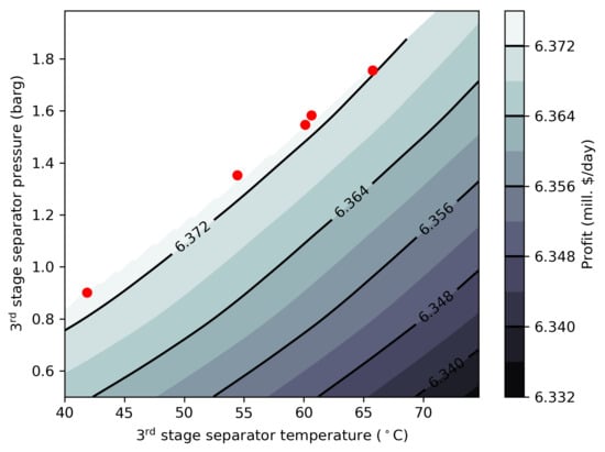
The correlation between the 3rd stage separator pressure and the 3rd stage separator temperature is further investigated in Figure 7. In the figure, the profit function (contour) is shown as a function of pressure and temperature in the separator as calculated by the surrogate models. The contour has been masked for profit functions where the RVP constraint is exceeded. The found optimal settings by the direct black-box optimization are shown as points. As seen from the figure, the profit iso-curves follows the shape of the RVP cut-off. This means that more or less equally good optimal conditions can be made with different 3rd stage separator pressure, as long as the corresponding temperature is changed accordingly to compensate, with higher pressure requiring higher temperatures in order not to violate the RVP constraint. Likewise, if the pressure is lowered, so shall the temperature be in order not to obtain sub-optimal profit.
Early attempts to predict the optimal middle separator pressure in a three stage separation train used the geometrical mean pressure i.e.,
The above Equation (8) results in equal pressure ratios between the various separator stages. Also, the geometric mean is smaller than the arithmetic mean pressure [8]. Al-Farhan et al. [8] discuss various correlations for predicting the optimal middle stage separator pressure and compare Equation (8), both with the method of Whinery and Campbell [3] and with optimization using thermodynamic flash calculations for a range of different fluid compositions and parameter settings. They observe that using the correlation of Whinery and Campbell for a crude oil almost always results in a third stage separator pressure being lower than the geometric mean. The same applies when performing optimization using flash calculations. These observations are consistent with the work of Ling et al. [6] and Bahadori et al. [7], who also find optimal values below the geometric mean/constant pressure ratio relation. The second stage separator pressures obtained in the present study is compared to the geometric mean value in Figure 8. As seen from the figure, in this study it is observed that the optimal second stage separator pressure can acquire values both near the geometric mean and below in agreement with the findings of others [6,7,8]. Interestingly it is also found that the optimal separator pressure can be significantly higher than the geometric mean value. It should be noted that the other referenced works [6,7,8] did neither include the flexibility of inter-stage heating, nor was condensate recycle streams from the compression system included. This added complexity and hence added degrees of freedom is likely responsible for this apparently more complex behavior in the present study. It also implies that care should be taken when optimizing separator pressures. It is not possible to do this independently of all other process parameters, and correlations developed for a simple separator train cannot necessarily be directly applied to a more realistic and complex process with both inter-stage heating and significant condensate recycle streams from the compression system and dew point control unit.
In order to evaluate the levels of expected improvements in case optimization is performed, the results of the present study is compared with previous similar studies. Obviously, the level of improvement highly depends on the starting point i.e., base case. Some processed are far from optimal parameter settings and some will be closer to optimal settings to begin with. Basically, this means that two studies using the same methods, the same process, parameter bounds, and constraints may conclude different potential improvements if the base case settings are different. Nevertheless, an attempt to quantify expected optimization improvements is provided in Table 7. In refs. [2,7,9,45] an improvement in terms of increased liquid production is explicitly stated compared to a non-optimized liquid production. The improvement observed in the present study is estimated using the difference between the base case and optimized profit cf. Table 2, Table 4 and Table 6. As seen from Table 7, it seems that separation train optimization may provide between approximately 0.1–2% increase in liquid production/operating profit depending on the process topology, fluid characterization, and base case level of optimization.
4. Conclusions
In the course of this study, the optimization of a realistic oil and gas separation plant has been investigated. Using DACE, utilizing LHS, and a rigorous process simulation model, surrogate models using Kriging have been established for selected model responses. The surrogate models have been used in combination with an evolutionary algorithm for optimizing the operating profit. The optimization is bounded in the variables and a constraint function is included to ensure that the optimal solution allows export of oil with an RVP < 12 psia.
It has been demonstrated that a surrogate model based on LHS and Kriging performs very well for optimizing an oil and gas separation plant. For some variables there seem to be unique settings, which are optimal. This mainly applies to the first stage separator pressure, which is optimal at its higher bound. The recovery of condensate from the dew point control unit is optimal when both the pressure and temperature is at the lower bound. The temperature in the compressor suction scrubber inlet (cooling) appears to be less sensitive in terms of applied settings. One of the more interesting findings in the present work is the fact that the pressure in the second and third stage separators apparently does not have unique optimal values. A range of third stage separator pressures may be equally optimal, as long as the temperature in the separator is also controlled. The higher the temperature the higher, yet more or less equally optimal, pressure and vice versa. The findings using the surrogate models for optimization is confirmed by black-box optimization by coupling the process simulation model directly to the optimization algorithm. The existence of multiple optimal separator pressures has not been observed in previous studies, where a unique optimal pressure for each separation stage is advocated.
The reason that this apparently more complex behavior, has not been seen previously, may be due to a number of reasons. Firstly, many previous studies did not take the compression system into account, and if doing so, often the normally recycled condensate streams were ignored, Further, inter-stage heating/cooling between the separation stages has also not been considered. Finally, many previous studies assume close to atmospheric pressure in the final separation stage (stock tank). For example, in many offshore installations the final separation stage is often at somewhat elevated pressure (two to three times atmospheric pressure), while the RVP export specification is controlled by the inlet temperature.
The implication of the results from the present study is that one should never focus only on finding optimal separator pressure settings when optimizing oil recovery/profit. One should always use a plant wide optimization approach and consider the entire process. There is a strong interplay between certain variables, which offers both some flexibility, but obviously also increases the number of variables that needs to be tuned.
Supplementary Materials
The following are available online at https://www.mdpi.com/2305-7084/4/1/11/s1. The LHS DACE plan, including simulation output, is available as supplementary material. The two process simulation file is also available as supplementary material.
Funding
This research received no external funding.
Acknowledgments
The author acknowledge Associate Professor Marco Maschietti, Section of Chemical Engineering, Department of Chemistry and Bioscience, the Faculty of Engineering and Science, Aalborg University Esbjerg, Denmark, and Assistant Professor Jan-Otto Hooghoudt, Department of Mathematical Sciences, The Faculty of Engineering and Science, Aalborg Univeristy, Denmark, for numerous enlightening discussions. Language secretary Susanne Tolstrup, Ramboll Energy, Field Development, is acknowledged for proof-reading the present manuscript.
Conflicts of Interest
The author declare no conflict of interest.
Abbreviations
The following abbreviations are used in this manuscript:
| BS&W | Basic Sediment & Water |
| ANN | Artificial Neural Network |
| C1 | Methane |
| C2 | Ethane |
| C3 | Propane |
| C4 | Butanes |
| C5 | Pentanes |
| CAPEX | Capital Expenditure |
| CM | Cooling Medium |
| CMA-ES | Covariance Matrix Adaptation Evolution Strategy |
| COM | Microsoft Component Object Model |
| COSTALD | Corresponding States Liquid Density |
| DACE | Design and Analysis of Computer Experiments |
| Efficiency | |
| FWHP | Flowing Wellhead Pressure |
| FWHT | Flowing Wellhead Temperature |
| GDE3 | The third evolution step of Generalized Differential Evolution |
| GOR | Gas Oil Ratio |
| HHV | Higher Heating Value |
| HM | Heating Medium |
| HP | High Pressure |
| LHS | Latin Hypercube Sampling |
| LHV | Lower Heating Value |
| LP | Low Pressure |
| LT | Low Temperature |
| -MOEA | epsilon-domination based Multi-Objective Evolutionary Algorithm |
| MP | Medium Pressure |
| MSE | Mean Square Error |
| NGL | Natural Gas Liquid |
| NPV | Net Present Value |
| NSGA | Non-dominated Sorting Genetic Algorithm |
| OPEX | Operating Expenditure |
| RVP | Reid Vapor Pressure |
| SLSQP | Sequential Least SQuares Programming |
| SPEA | Strength Pareto Evolutionary Algorithm |
| SW | Seawater |
| TVP | True Vapor Pressure |
| VBA | Visual Basic for Applications |
References
- Kim, I.H.; Dan, S.; Kim, H.; Rim, H.R.; Lee, J.M.; Yoon, E.S. Simulation-Based Optimization of Multistage Separation Process in Offshore Oil and Gas Production Facilities. Ind. Eng. Chem. Res. 2014, 53, 21. [Google Scholar] [CrossRef]
- Ghaedi, M.; Ebrahimi, A.N.; Pishvaie, M.R. Application of Genetic Algorithm for Optimization of Separator Pressures in Multistage Production Units. Chem. Eng. Commun. 2014, 201, 926–938. [Google Scholar] [CrossRef]
- Whinery, K.F.; Campbell, J.M. A Method for Determining Optimum Second Stage Pressure in Three Stage Separation. J. Petroleum Technol. 1958, 10, 53–54. [Google Scholar] [CrossRef]
- Al-Jawad, M.S.; Hassan, O.F. Correlations for Optimum Separation Pressures For Sequential Field Separation System—SPE-118225-MS; Society of Petroleum Engineers: Abu Dhabi, UAE, 2008; p. 13. [Google Scholar] [CrossRef]
- Al-Jawad, M.S.; Hassan, O.F. Correlating Optimum Stage Pressure for Sequential Separator Systems. SPE Proje. Facil. Constr. 2010, 5, 13–16. [Google Scholar] [CrossRef]
- Ling, K.; Wu, X.; Guo, B.; He, J. New Method To Estimate Surface-Separator Optimum Operating Pressures. Oil Gas Facil. 2013, 2, 65–76. [Google Scholar] [CrossRef]
- Bahadori, A.; Vuthaluru, H.B.; Mokhatab, S. Optimizing separator pressures in the multistage crude oil production unit. Asia-Pac. J. Chem. Eng. 2008, 3, 380–386. [Google Scholar] [CrossRef]
- Al-Farhan, F.A.; Luis, F.A.H. Optimization of surface condensate production from natural gases using artificial intelligence. J. Pet. Sci. Eng. 2006, 53, 135–147. [Google Scholar] [CrossRef]
- Motie, M.; Moein, P.; Moghadasi, R.; Hadipour, A. Separator Pressure Optimisation and Cost Evaluation of a Multistage Production Unit Using Genetic Algorithm. In Proceedings of the IPTC-19396-MS International Petroleum Technology Conference, Beijing, China, 27–29 March 2019; p. 14. [Google Scholar] [CrossRef]
- Andreasen, A.; Rasmussen, K.R.; Mandø, M. Plant Wide Oil and Gas Separation Plant Optimisation using Response Surface Methodology. In Proceedings of the 3rd IFAC Workshop on Automatic Control in Offshore Oil and Gas Production OOGP, Esbjerg, Denmark, 30 May–1 June 2018; pp. 178–184. [Google Scholar] [CrossRef]
- Peng, D.Y.; Robinson, D.B. A New Two-Constant Equation of State. Ind. Eng. Chem. Fundam. 1976, 15, 59–64. [Google Scholar] [CrossRef]
- Hankinson, R.W.; Thomson, G.H. A new correlation for saturated densities of liquids and their mixtures. AIChE J. 1979, 25, 653–663. [Google Scholar] [CrossRef]
- Price, B. (Ed.) GPSA Engineering Data Book, 13th ed.; Gas Processors Suppliers Association: Tulsa, OK, USA, 2012; Volume I–II. [Google Scholar]
- Mckay, M.D.; Beckman, R.J.; Conover, W.J. A Comparison of Three Methods for Selecting Values of Input Variables in the Analysis of Output from a Computer Code. Technometrics 2000, 42, 55–61. [Google Scholar] [CrossRef]
- Morris, M.D.; Mitchell, T.J. Exploratory designs for computational experiments. J. Stat. Plan. Inference 1995, 43, 381–402. [Google Scholar] [CrossRef] [Green Version]
- Paulson, C.; Ragkousis, G. pyKriging: A Python Kriging Toolkit. 2015. Available online: https://zenodo.org/record/21389 (accessed on 5 February 2002). [CrossRef]
- Loeppky, J.L.; Sacks, J.; Welch, W.J. Choosing the Sample Size of a Computer Experiment: A Practical Guide. Technometrics 2009, 51, 366–376. [Google Scholar] [CrossRef] [Green Version]
- Afzal, A.; Kim, K.Y.; won Seo, J. Effects of Latin hypercube sampling on surrogate modeling and optimization. Int. J. Fluid Mach. Syst. 2017, 10, 240–253. [Google Scholar] [CrossRef]
- Ibrahim, M.; Al-Sobhi, S.; Mukherjee, R.; AlNouss, A. Impact of Sampling Technique on the Performance of Surrogate Models Generated with Artificial Neural Network (ANN): A Case Study for a Natural Gas Stabilization Unit. Energies 2019, 12, 1906. [Google Scholar] [CrossRef] [Green Version]
- AspenTech. Aspen HYSYS Customization, Ver. 10; Aspen Technology Inc.: Bedford, MA, USA, 2017. [Google Scholar]
- Aspelund, A.; Gundersen, T.; Myklebust, J.; Nowak, M.; Tomasgard, A. An optimization-simulation model for a simple LNG process. Comput. Chem. Eng. 2010, 34, 1606–1617. [Google Scholar] [CrossRef]
- Caballero, J.A.; Grossmann, I.E. An algorithm for the use of surrogate models in modular flow sheet optimization. AIChE J. 2008, 54, 2633–2650. [Google Scholar] [CrossRef]
- Krige, D. A Statitical Approach to some Mine Valuation and Allied Problems on the Witwatersrand. Master’s Thesis, University of the Witwatersrand, Johannesburg, South Africa, 1951. [Google Scholar]
- Matheron, G. Principles of geostatistics. Econ. Geol. 1963, 58, 1246–1266. [Google Scholar] [CrossRef]
- Jones, D.R. A Taxonomy of Global Optimization Methods Based on Response Surfaces. J. Glob. Optim. 2001, 21, 345–383. [Google Scholar] [CrossRef]
- Ragkousis, G.E.; Curzen, N.; Bressloff, N.W. Multi-objective optimisation of stent dilation strategy in a patient-specific coronary artery via computational and surrogate modelling. J. Biomech. 2016, 49, 205–215. [Google Scholar] [CrossRef] [Green Version]
- Paulson, C. The Rapid Development of Bespoke Sensorcraft: A Proposed Design Loop for Small Unmanned Aircraft. Ph.D. Thesis, University of Southampton, Southampton, UK, 2017. [Google Scholar]
- Davis, E.; Ierapetritou, M. A kriging method for the solution of nonlinear programs with black-box functions. AIChE J. 2007, 53, 2001–2012. [Google Scholar] [CrossRef]
- Quirante, N.; Javaloyes, J.; Ruiz-Femenia, R.; Caballero, J.A. Optimization of Chemical Processes Using Surrogate Models Based on a Kriging Interpolation. In Proceedings of the 12th International Symposium on Process Systems Engineering and 25th European Symposium on Computer Aided Process Engineering, Copenhagen, Denmark, 31 May–4 June 2015; Gernaey, K.V., Huusom, J.K., Gani, R., Eds.; Elsevier: Amsterdam, The Netherlands, 2015; pp. 179–184. [Google Scholar] [CrossRef] [Green Version]
- Oliphant, T.E. Guide to NumPy, 2nd ed.; CreateSpace Independent Publishing Platform: Scotts Valley, CA, USA, 2015. [Google Scholar]
- Walt, S.V.D.; Colbert, S.C.; Varoquaux, G. The NumPy Array: A Structure for Efficient Numerical Computation. Comp. Sci. Eng. 2011, 13, 22–30. [Google Scholar] [CrossRef] [Green Version]
- Jones, E.; Oliphant, T.; Peterson, P. SciPy: Open source scientific tools for Python. Available online: http://www.scipy.org/ (accessed on 4 February 2020).
- Hunter, J.D. Matplotlib: A 2D graphics environment. Comp. Sci. Eng. 2007, 9, 90–95. [Google Scholar] [CrossRef]
- Ochoa-Estopier, L.; Enriquez Gutierrez Victor, M.; Chen, L.; Fernandez-Ortiz, J.; Herrero-Soriano, L.; Jobson, M. Industrial Application of Surrogate Models to Optimize Crude Oil Distillation Units. Chem. Eng. Trans. 2018, 69, 289–294. [Google Scholar] [CrossRef]
- Djikpéssé, H.; Couët, B.; Wilkinson, D. A practical sequential lexicographic approach for derivative-free black-box constrained optimization. Eng. Optim. 2011, 43, 721–739. [Google Scholar] [CrossRef]
- Emissions to Air. Available online: https://www.norskpetroleum.no/en/environment-and-technology/emissions-to-air/ (accessed on 4 February 2020).
- Deb, K.; Pratap, A.; Agarwal, S.; Meyarivan, T. A fast and elitist multiobjective genetic algorithm: NSGA-II. IEEE Trans. Evolut. Comput. 2002, 6, 182–197. [Google Scholar] [CrossRef] [Green Version]
- Kukkonen, S.; Lampinen, J. GDE3: The third evolution step of generalized differential evolution. In Proceedings of the IEEE Congress on Evolutionary Computation, Edinburgh, Scotland, UK, 2–5 September 2005; Volume 1, pp. 443–450. [Google Scholar] [CrossRef]
- Zitzler, E.; Laumanns, M.; Thiele, L. SPEA2: Improving the Strength Pareto Evolutionary Algorithm; Technical report; Computer Engineering and Networks Laboratory (TIK) Department of Electrical Engineering, Swiss Federal Institute of Technology (ETH): Zurich, Switzerland, 2001. [Google Scholar]
- Deb, K.; Mohan, M.; Mishra, S. A Fast Multi-objective Evolutionary Algorithm for Finding Well-Spread Pareto-Optimal Solutions. KanGAL Rep. 2003, 2003002, 1–18. [Google Scholar]
- Hansen, N. The CMA Evolution Strategy: A Comparing Review. In Towards a New Evolutionary Computation. Advances on Estimation of Distribution Algorithms; Lozano, J., Larranaga, P., Inza, I., Bengoetxea, E., Eds.; Springer: Berlin, Germeny, 2006; pp. 75–102. [Google Scholar]
- Deb, K.; Jain, H. An Evolutionary Many-Objective Optimization Algorithm Using Reference-Point-Based Nondominated Sorting Approach, Part I: Solving Problems With Box Constraints. IEEE Trans. Evolut. Comput. 2014, 18, 577–601. [Google Scholar] [CrossRef]
- Hadka, D. Platypus—A Free and Open Source Python Library for Multiobjective Optimization. Available online: https://github.com/Project-Platypus/Platypus (accessed on 4 February 2020).
- Kraft, D. Algorithm 733: TOMP–Fortran Modules for Optimal Control Calculations. ACM Trans. Math. Softw. 1994, 20, 262–281. [Google Scholar] [CrossRef]
- Kylling, Ø.W. Optimizing separator pressure in multistage crude oil production plant. Master’s Thesis, Norwegian University of Science and Technology, Trondheim, Norway, 2009. [Google Scholar]
Figure 1.
Processflow diagram implemented in the process simulator flow sheet.

Figure 2.
Phase envelopes for the applied well fluid.

Figure 3.
Calculationflow for Latin-Hypercube sampling using the process simulation.

Figure 4.
Convergence of objection function and variables as a function of generation number for surrogate models with the Non-dominated Sorting Genetic Algorithm (NSGA-II) algorithm.
Figure 4.
Convergence of objection function and variables as a function of generation number for surrogate models with the Non-dominated Sorting Genetic Algorithm (NSGA-II) algorithm.


Figure 5.
Convergence of variables and constraint function as a function of generation number for surrogate models with the NSGA-II algorithm.
Figure 5.
Convergence of variables and constraint function as a function of generation number for surrogate models with the NSGA-II algorithm.


Figure 6.
Profitfunction as a function of 2nd and 3rd stage separator pressure using the surrogate model. Objective function calculated with 52 C and 32 barg in the 1st stage separator, 25 C in all compressor suction scrubbers, 60 barg after the HP compressor, and −5 C in the refrigeration/dew point control unit. The profit function has been masked for Reid Vapor Pressure (RVP) > 12 psia. The upper figure is obtained with a 3rd stage separator temperature of 40 C, and the lower figure with 60 C.

Figure 7.
Profitfunction as a function of 3rd stage separator pressure and temperature. Profit function contour calculated using the average settings from the optimization for all other parameters cf. Figure 6. Red points are the optimal settings from the direct black-box optimization. Profit function has been masked for RVP > 12 psia.

Figure 8.
Optimal 2nd stage separator pressure as a function of the geometric mean separator pressure. Points shown for both optimal settings found using surrogate models as well as using the full black-box process simulation model.
Figure 8.
Optimal 2nd stage separator pressure as a function of the geometric mean separator pressure. Points shown for both optimal settings found using surrogate models as well as using the full black-box process simulation model.


Table 1.
Wellfluid composition and hypothetical characterization for the investigated well fluid [7].
Table 1.
Wellfluid composition and hypothetical characterization for the investigated well fluid [7].
| Pseudo-Component | |||
|---|---|---|---|
| Component | Mole Fraction (%) | Molecular Weight (kg/kmole) | Specific Gravity (–) |
| HO | 0.0 | ||
| N | 0.0 | ||
| CO | 1.5870 | ||
| CH | 52.51 | ||
| CH | 6.24 | ||
| CH | 4.23 | ||
| i-CH | 0.855 | ||
| n-CH | 2.213 | ||
| i-CH | 1.1240 | ||
| n-CH | 1.271 | ||
| n-CH | 2.2890 | ||
| C-CUT1 | 0.8501 | 108.47 | 0.7411 |
| C-CUT2 | 1.2802 | 120.4 | 0.755 |
| C-CUT3 | 1.6603 | 133.63 | 0.7695 |
| C-CUT4 | 6.5311 | 164.79 | 0.799 |
| C-CUT5 | 6.3311 | 215.94 | 0.8387 |
| C-CUT6 | 4.9618 | 274.34 | 0.8754 |
| C-CUT7 | 2.9105 | 334.92 | 0.90731 |
| C-CUT8 | 3.0505 | 412.79 | 0.9575 |
Table 2.
Processsimulation parameter settings for base case simulations. The gas export pressure was set to 188 barg for all simulations.
Table 2.
Processsimulation parameter settings for base case simulations. The gas export pressure was set to 188 barg for all simulations.
| Bounds | ||||
|---|---|---|---|---|
| Parameters | Unit | Base Case | Low | High |
| Profit | ($/day) | 6,307,920 | – | – |
| Oil | (m/d) | 15,905 | – | – |
| Power | (kW) | 12,019 | – | – |
| RVP | (psia) | 10.08 | – | – |
| T | ( C) | 70 | 50 | 70 |
| P | (barg) | 32 | 11 | 32 |
| P | (barg) | 8 | 2.5 | 10 |
| T | ( C) | 65 | 40 | 75 |
| P | (barg) | 1.5 | 0.5 | 2 |
| T | ( C) | 32 | 25 | 40 |
| T | ( C) | 32 | 25 | 40 |
| T | ( C) | 32 | 25 | 40 |
| P | (barg) | 90 | 60 | 90 |
| T | ( C) | 10 | −5 | 28 |
Table 3.
Applied modeling details for unit operations. For 20-HA-02 the duty is assumed to be zero i.e., no inter-stage heating applied between first and second separation stage. A fixed temperature is applied for the discharge of the dehydration inlet cooler, 24-HA-01, of 30 C.
Table 3.
Applied modeling details for unit operations. For 20-HA-02 the duty is assumed to be zero i.e., no inter-stage heating applied between first and second separation stage. A fixed temperature is applied for the discharge of the dehydration inlet cooler, 24-HA-01, of 30 C.
| (bar) | |
|---|---|
| 20-HA-01 | 0.5 |
| 20-HA-03 | 0.5 |
| 21-HA-01 | 0.5 |
| 23-HA-01 | 0.3 |
| 23-HA-02 | 1.0 |
| 23-HA-03 | 1.0 |
| 24-HA-01 | 1.0 |
| 25-HA-01 | 0.5 |
| 25-HA-02 | 0.5 |
| 27-HA-01 | 0.0 |
Table 4.
Resultsfor main objective function, constraint function, supporting responses, and model variables from 10 consecutive runs using surrogate models in the NSGA-II algorithm.
Table 4.
Resultsfor main objective function, constraint function, supporting responses, and model variables from 10 consecutive runs using surrogate models in the NSGA-II algorithm.
| Run No. | |||||||||||||
|---|---|---|---|---|---|---|---|---|---|---|---|---|---|
| 1 | 2 | 3 | 4 | 5 | 6 | 7 | 8 | 9 | 10 | Mean | (%) | ||
| Profit (mill. $/d) | 6.3751 | 6.3751 | 6.3738 | 6.3726 | 6.3749 | 6.3751 | 6.3751 | 6.3748 | 6.3751 | 6.3749 | 6.3747 | 8.0 × 10 | 0.013 |
| RVP (psia) | 12.00 | 12.00 | 12.00 | 12.00 | 12.00 | 12.00 | 12.00 | 12.00 | 12.00 | 12.00 | 12.00 | 3.1 × 10 | 0.003 |
| Oil (Sm3/d) | 16,137.6 | 16,137.2 | 16,135.3 | 16,133.8 | 16,136.0 | 16,137.3 | 16,136.2 | 16,135.5 | 16,136.9 | 16,136.0 | 16,136.2 | 1.1 | 0.007 |
| Power (kW) | 13,599 | 13,597 | 13,627 | 13,672 | 13,305 | 13,580 | 13,391 | 13,285 | 13,557 | 13,280 | 13,489 | 156 | 1.154 |
| Tsep1 ( C) | 50.72 | 51.29 | 52.63 | 51.89 | 51.07 | 51.02 | 51.54 | 51.20 | 51.30 | 50.96 | 51.36 | 0.55 | 1.07 |
| Psep1 (barg) | 32.00 | 32.00 | 32.00 | 32.00 | 32.00 | 32.00 | 31.99 | 31.99 | 32.00 | 32.00 | 32.00 | 0.00 | 0.01 |
| Psep2 (barg) | 7.84 | 7.86 | 7.69 | 5.18 | 7.96 | 7.87 | 7.87 | 7.96 | 7.85 | 7.82 | 7.59 | 0.85 | 11.21 |
| Tsep3 ( C) | 41.85 | 42.15 | 62.52 | 67.56 | 44.99 | 41.76 | 42.10 | 44.97 | 41.88 | 43.58 | 47.34 | 9.49 | 20.04 |
| Psep3 (barg) | 0.89 | 0.90 | 1.64 | 1.83 | 1.00 | 0.89 | 0.91 | 1.00 | 0.90 | 0.96 | 1.09 | 0.34 | 31.45 |
| Tscrub1 ( C) | 39.79 | 39.97 | 39.99 | 33.79 | 31.13 | 39.71 | 33.67 | 30.02 | 37.73 | 29.80 | 35.56 | 4.33 | 12.19 |
| Tscrub2 ( C) | 25.00 | 25.01 | 25.00 | 25.00 | 25.00 | 25.00 | 25.00 | 25.03 | 25.00 | 25.00 | 25.01 | 0.01 | 0.03 |
| Tscrub3 ( C) | 28.03 | 26.93 | 27.70 | 28.27 | 27.98 | 25.52 | 28.33 | 37.46 | 27.98 | 28.32 | 28.65 | 3.21 | 11.22 |
| Pboost (barg) | 60.00 | 60.00 | 60.00 | 60.00 | 60.00 | 60.00 | 60.00 | 60.00 | 60.00 | 60.00 | 60.00 | 0.00 | 0.00 |
| Trefrig ( C) | −5.00 | −5.00 | −5.00 | −5.00 | −5.00 | −5.00 | −5.00 | −5.00 | −5.00 | −5.00 | −5.00 | 0.00 | −0.01 |
Table 5.
Processsimulation output using the 10 NSGA-II optimal solutions found using the surrogate models cf. Table 4.
Table 5.
Processsimulation output using the 10 NSGA-II optimal solutions found using the surrogate models cf. Table 4.
| Run | Profit (Mill. Dollars/Day) | RVP (psia) | Oil (Sm3/d) | Power (kW) |
|---|---|---|---|---|
| 1 | 6.3749 | 12.00 | 16,137 | 13,617 |
| 2 | 6.3745 | 11.99 | 16,136 | 13,605 |
| 3 | 6.3728 | 11.93 | 16,130 | 13,543 |
| 4 | 6.3724 | 11.93 | 16,128 | 13,613 |
| 5 | 6.3743 | 11.97 | 16,133 | 13,416 |
| 6 | 6.3746 | 11.99 | 16,136 | 13,609 |
| 7 | 6.3741 | 11.99 | 16,134 | 13,489 |
| 8 | 6.3732 | 11.95 | 16,131 | 13,397 |
| 9 | 6.3746 | 12.00 | 16,136 | 13,569 |
| 10 | 6.3735 | 11.97 | 16,132 | 13,401 |
| Mean | 6.3739 | 11.97 | 16,133 | 13,526 |
| Std. Dev. | 0.000857478 | 0.025 | 2.907 | 92.477 |
| Std. Dev. (%) | 0.013452961 | 0.205 | 0.018 | 0.684 |
Table 6.
Profitmaximum obtained by optimization of the black-box model (process simulation) directly using the NSGA-II algorithm.
Table 6.
Profitmaximum obtained by optimization of the black-box model (process simulation) directly using the NSGA-II algorithm.
| Run No. | ||||||||
|---|---|---|---|---|---|---|---|---|
| 1 | 2 | 3 | 4 | 5 | Mean | Std. Dev. | Std. Dev. (%) | |
| Profit | 6.3753 | 6.3735 | 6.3741 | 6.3739 | 6.3739 | 6.3741 | 0.0007 | 0.010 |
| RVP | 11.99 | 12.00 | 12.00 | 12.00 | 12.00 | 12.00 | 0.0022 | 0.018 |
| Tsep1 | 50.6 | 53.4 | 54.7 | 52.0 | 50.0 | 52.1 | 1.9 | 3.707 |
| Psep1 | 31.2 | 31.6 | 31.6 | 31.1 | 31.3 | 31.4 | 0.2 | 0.713 |
| Psep2 | 8.21 | 6.46 | 7.05 | 6.70 | 5.42 | 6.77 | 1.01 | 14.92 |
| Tsep3 | 41.85 | 60.63 | 54.43 | 60.10 | 65.75 | 56.55 | 9.14 | 16.17 |
| Psep3 | 0.90 | 1.58 | 1.35 | 1.55 | 1.76 | 1.43 | 0.33 | 22.91 |
| Tscrub1 | 34.74 | 32.99 | 35.07 | 39.46 | 38.84 | 36.22 | 2.80 | 7.72 |
| Tscrub2 | 30.98 | 32.71 | 26.07 | 27.42 | 25.01 | 28.44 | 3.28 | 11.54 |
| Tscrub3 | 36.46 | 32.26 | 29.77 | 38.34 | 33.28 | 34.02 | 3.40 | 10.00 |
| Pboost | 60.95 | 60.48 | 60.42 | 60.14 | 60.11 | 60.42 | 0.34 | 0.56 |
| Trefrig | −4.99 | −4.99 | −5.00 | −4.99 | −4.99 | −4.99 | 0.00 | −0.06 |
© 2020 by the author. Licensee MDPI, Basel, Switzerland. This article is an open access article distributed under the terms and conditions of the Creative Commons Attribution (CC BY) license (http://creativecommons.org/licenses/by/4.0/).
Share and Cite
MDPI and ACS Style
Andreasen, A. Applied Process Simulation-Driven Oil and Gas Separation Plant Optimization Using Surrogate Modeling and Evolutionary Algorithms. ChemEngineering 2020, 4, 11. https://doi.org/10.3390/chemengineering4010011
AMA Style
Andreasen A. Applied Process Simulation-Driven Oil and Gas Separation Plant Optimization Using Surrogate Modeling and Evolutionary Algorithms. ChemEngineering. 2020; 4(1):11. https://doi.org/10.3390/chemengineering4010011
Chicago/Turabian StyleAndreasen, Anders. 2020. "Applied Process Simulation-Driven Oil and Gas Separation Plant Optimization Using Surrogate Modeling and Evolutionary Algorithms" ChemEngineering 4, no. 1: 11. https://doi.org/10.3390/chemengineering4010011